Spatiotemporal Evolution of Ecological Environment Quality and Driving Factors in Jiaodong Peninsula, China

Abstract

To monitor the Ecological Environment Quality (EEQ) of the Jiaodong Peninsula and provide a scientific basis for ecological environment governance and sustainable development in the region, this study evaluates the EEQ of Jiaodong using the Remote Sensing-based Ecological Index (RSEI) model and analyzes its spatiotemporal evolution patterns, building upon single-factor correlation analysis using the Random Sample Consensus (RANSAC) algorithm, using GeoDetector to analyze the driving mechanisms of human activities and natural factors in EEQ. The results indicate the following: (1) The average RSEI values for 2000, 2010, and 2020 are 0.60, 0.57, and 0.66, with Good or Excellent areas accounting for 56.48%, 51.02%, and 67.17%. From 2000 to 2020, RSEI strong improvement areas were predominantly distributed in the eastern hilly areas of the Jiaodong Peninsula. The RSEI of the Jiaodong Peninsula showed significant spatial autocorrelation. (2) The RANSAC algorithm effectively reduces noise interference in remote sensing data, thereby improving the accuracy of single-factor correlation analysis. (3) In 2000, the importance of natural factors exceeds that of human activity factors. The Standardized Precipitation Evapotranspiration Index (SPEI) is the most important driving factor; while in 2010 and 2020, human activity factors surpass natural factors in importance, with the Land Use Composite Index (LUCI) being the most significant driving factor. The driving factors exhibited double-factor and nonlinear enhancement. The most significant interaction factors affecting the EEQ of the Jiaodong Peninsula in 2000, 2010, and 2020 are SPEI∩GDP, LUCI∩SPEI, and LUCI∩GDP.

1. Introduction

In recent years, under the influences of human activities and climate change, the exhaustion of natural resources, environmental pollution, biodiversity decline, and the rising frequency of extreme weather events like droughts and floods have posed serious threats to the balance of ecosystems and the sustainable development of human society [1,2,3,4]. Based on diverse research perspectives including ecosystem services [5], ecological vulnerability [6], ecological security patterns [7], and ecological carrying capacity [8], the monitoring and assessment of changes in Ecological Environment Quality (EEQ) and its driving mechanisms have become essential for governments and ecological conservation organizations to formulating ecological conservation policies.

Xu H. Q. [9] introduced the Remote Sensing Ecological Index (RSEI), which evaluates EEQ by integrating four indicators—wetness, greenness, heat, and dryness—through principal component analysis (PCA). Compared to methods using single indicators such as the normalized difference vegetation index (NDVI) [10] or Leaf Area Index (LAI) [11] for assessing EEQ, the RSEI contain more comprehensive information. The RSEI has been widely applied in evaluating EEQ in urban ecosystems [12,13], natural ecosystems [14,15], and key ecological conservation areas [16] at different scales.

There are two limitations that can impact the assessment results of RSEI. First, the underlying data of RSEI rely on remote sensing images, where variations in sensors and acquisition times can lead to pseudofluctuations. Challenges like cloud cover, periodic stripes, bright lines, and spots make significant noise interference, substantially influencing the results of the driving analysis [17,18]. Second, ecosystems, especially urban ones, are influenced by the combined effects of natural, social, and economic factors [19]. Natural and human factors are interwoven in ecosystem components, integrated in structure, coupled in processes, complementary in functions, and synergistic in services. Therefore, traditional correlation analysis and regression analysis have limitations in quantifying the contributions of driving factors to EEQ and their interactions.

The Jiaodong Peninsula, characterized as a complex coastal ecosystem, benefits from favorable climatic conditions and abundant natural resources, experiencing significant human activity. Over the past two decades, the region has become one of the fastest-growing urban agglomerations in northern China, associated with increasing vulnerability to coastal erosion, fragmented landscapes in ecological source areas, and declining biodiversity [20,21]. According to Huang et al., there was a significant decrease of 16.8% in the ecological resilience of the Shandong Peninsula region from 2000 to 2018 [22]. Intense human activities [23,24] and extreme weather events [25] have posed significant challenges to the ecological balance of the Jiaodong Peninsula. Using RSEI to assess the historical and current status of the EEQ in Jiaodong Peninsula, exploring the driving mechanisms of human activities and natural elements, is crucial for formulating targeted local ecological conservation policies and enhancing the resilience of the complex coastal ecosystem of the Jiaodong Peninsula to disturbances.

To overcome the issues associated with conducting ecological assessments based on remote sensing images, this research using the Random Sample Consensus Algorithm (RANSAC) proposed by Fischler and Bolles in 1981 to address the impact of remote sensing noise on correlation analysis. RANSAC exhibits strong robustness to noisy data, and has been widely applied in measurement engineering, image matching, and point cloud orientation [26,27]. GeoDetector is a statistical method for detecting spatial differentiation and revealing the driving forces behind it [28], which can identify the interactions between driving factors and has been well applied in the analysis of EEQ driving factors [29,30].

The objectives of this study are (1) to evaluate the EEQ of the Jiaodong Peninsula from 2000 to 2020 using the RSEI model and analyze spatial clustering characteristics through LISA clustering; (2) to comprehensively analyze the relative contributions of human activities and natural factors to EEQ using RANSAC and GeoDetector, providing references for promoting the green and high-quality growth of the Jiaodong Peninsula urban agglomeration.

2. Materials and Methods

2.1. Research Area

The Jiaodong Peninsula is located in the eastern coastal region of the Shandong Peninsula, China (${118}^{\circ }{10}^{\prime }$–${122}^{\circ }{42}^{\prime }$ E, ${35}^{\circ }{04}^{\prime }$–${38}^{\circ }{23}^{\prime }$ N), situated between the Bohai Sea and the Yellow Sea (Figure 1). It encompasses five cities—Weifang, Qingdao, Rizhao, Yantai, and Weihai—comprising 41 districts and counties. With a land area of approximately 52,000 km² and a population of around 32.43 million permanent residents, the urbanization rate stands at 67%, contributing to a regional GDP of approximately 3.1 trillion yuan. The Jiaodong Peninsula urban agglomeration experiences a temperate monsoon climate with distinct maritime characteristics, featuring four distinct seasons and concurrent rainy and hot periods. The topography of the Jiaodong Peninsula predominantly consists of low mountains and hills, with vegetation primarily comprising deciduous broadleaved forests and areas of artificial vegetation. As one of China’s most developed regions, the Jiaodong Peninsula urban agglomeration holds significant importance in the national strategic framework for ecological protection and high-quality development within the Yellow River Basin.

2.2. Data Sources and Processing

The Landsat images dataset for growing seasons (June to September) of the years 2000, 2010, and 2020, collected and processed by the Google Earth Engine platform (https://developers.google.com/earth-engine/datasets, accessed on 18 January 2020) was used to calculate the RSEI. The selected images are complete and free from gap-filling. The CFMASK algorithm available on the GEE platform was used for cloud masking, the permanent water area band from the JRC Global Surface Water Distribution dataset was used for water masking. The Landsat images of the study area were mosaicked and RSEI was calculated using median fusion. The spatial resolution of the output remote sensing images is 30 m. Details of Landsat images are shown in

Table 1. Landsat images information.

Year	Source	Dates of the Landsat Images (M-D)	The Maximum Cloud Amount
2000	Landsat 5/7	Landsat 5: 6-4, 6-6, 6-11, 6-13, 7-22, 7-24, 7-31, 8-14, 9-8, 9-10, 9-15, 9-17, 9-26 Landsat 7: 6-5, 6-12, 6-28, 6-30, 7-14, 7-21, 7-30, 8-01, 8-06, 8-17, 8-22, 9-9, 9-16, 9-18	40%
2010	Landsat 5	6-7, 6-25, 7-11, 8-3, 8-17, 8-19, 8-25, 9-11, 9-13, 9-26	20%
2020	Landsat 8	6-4, 6-25, 6-27, 7-15, 7-20, 7-29, 8-28, 8-30, 9-06	20%

.

This study selected six driving factors, encompassing both natural and human activity elements, as independent variables. The data sources used for computing these variables are shown in

Table 2. Data sources for driving factors.

Data	Source	Spatial Resolution	URL
Land Cover	30 m annual land cover and its dynamics in China from 1990 to 2019	30 m	https://zenodo.org/records/4417810, accessed on 18 January 2024
Population Density	WordPop	1 km	https://www.worldpop.org/
Gross Domestic Product (GDP)	Resource and Environmental Science and Data Center	1 km	https://www.resdc.cn/
Precipitation	The National Tibetan Plateau Data Center	1 km	https://data.tpdc.ac.cn/
Temperature	The National Tibetan Plateau Data Center	1 km	https://data.tpdc.ac.cn/
Evaporation	The National Tibetan Plateau Data Center	1 km	https://data.tpdc.ac.cn/

.

2.3. Method

2.3.1. Construction of RSEI

This study evaluates the EEQ of the Jiaodong Peninsula from 2000 to 2020 based on the RSEI. According to Xu’s [9] framework, principal component analysis (PCA) is employed to combine four ecological indicators (wetness, greenness, heat, and dryness), with the first principal component (PC1) utilized to construct RSEI. The weights of each indicator are objectively determined based on their contributions to PC1, which rely on the data characteristics of each study area rather than subjective factors [31].

$$RSEI=\left[f(Wetness,\mathrm{Greenness},Heat,Dryness)\right]$$

(1)

Explanation and details of the four indicators, computed using related thematic remote sensing indices/algorithms, are listed as follows:

(1)

Wetness indicator: Wet component, applying the tasseled cap transformation to the original landsat date [32,33], can effectively reflect soil and vegetation moisture information. The formula is as follows:

$$WET={\alpha }_1{\beta }_{blue}+{\alpha }_2{\beta }_{green}+{\alpha }_3{\beta }_{red}+{\alpha }_4{\beta }_{nir}-{\alpha }_5{\beta }_{swir1}-{\alpha }_6{\beta }_{swir2},$$

(2)

where ${\beta }_{blue}$, ${\beta }_{green}$, ${\beta }_{red}$, ${\beta }_{nir}$, ${\beta }_{swir1}$, and ${\beta }_{swir2}$ represent the reflectance values of the blue, green, red, near-infrared, short-wave infrared 1, and short-wave infrared 2 bands, respectively. $\alpha$ is a weight coefficient. For Landsat TM data, these coefficients are $0.0315$, $0.2021$, $0.3012$, $0.1594$, $0.6806$, and $0.6109$ [34]. For Landsat-8 OLI data, they are $0.1511$, $0.1973$, $0.3283$, $0.3407$, $0.7117$, and $0.4559$ [35].

(2)

Greenness indicator: This indicator can reflect the vegetation coverage and growth conditions of study area. Greenness is expressed by Normalized Difference Vegetation Index (NDVI) [36]. The formula is as follows:

$$NDVI=\frac{{\beta }_{nir}-{\beta }_{red}}{{\beta }_{nir}+{\beta }_{red}},$$

(3)

(3)

Heat indicator: This component, expressed by Land Surface Temperature (LST), reflects the surface temperature of urban underlying surfaces, which is directly related to the quality of human habitation and energy consumption [37]. The formula is as follows:

$$LST=\frac{T}{1+(\lambda T/\delta )ln\left(ϵ\right)},$$

(4)

where $\lambda$ is the central wavelength of the thermal infrared band, $\delta =1.438\times {10}^{-2}$ m·k, and $ϵ$ is the ground emissivity. $L=gain\times DN+bias$ and $T=\frac{K_2}{ln(K_1/L+1)}$, where $gain$, $DN$, and $bias$ represent the gain value of the thermal infrared band, the grayscale value of the pixel, and the bias value of the thermal infrared band; $K_1$ and $K_2$ are calibration parameters.

(4)

Dryness indicator: This component is used to reflect the built area of the region [38]. The normalized difference built-up and soil index (NDBSI) can be represented by synthesizing the bare soil index (SI) and the impervious built-up index (IBI). The formula is as follows:

$$NDBSI=\frac{SI+IBI}{2},$$

(5)

$$SI=\frac{({\beta }_{swir1}+{\beta }_{red})-({\beta }_{nir}+{\beta }_{blue})}{({\beta }_{swir1}+{\beta }_{red})+({\beta }_{nir}+{\beta }_{blue})},$$

(6)

$$IBI=\frac{\frac{2{\beta }_{swir1}}{{\beta }_{swir1}+{\beta }_{nir}}-[\frac{{\beta }_{nir}}{{\beta }_{nir}+{\beta }_{red}}+\frac{{\beta }_{green}}{{\beta }_{green}+{\beta }_{swir1}}]}{\frac{2{\beta }_{swir1}}{{\beta }_{swir1}+{\beta }_{nir}}+[\frac{{\beta }_{nir}}{{\beta }_{nir}+{\beta }_{red}}+\frac{{\beta }_{green}}{{\beta }_{green}+{\beta }_{swir1}}]},$$

(7)

Four indicators are normalized according to Formula (8) to remove dimensional inconsistencies.

$$B{I}_i=\frac{B_i-B_{min}}{B_{max}-B_{min}},$$

(8)

$B{I}_i$ represents the normalized indicator, $B_i$ represents the original indicator, and $B_{max}$ and $B_{min}$ are the maximum and minimum values of the indicator.

It is generally considered that principal components with contribution values exceeding 70% are sufficient for constructing an effective RSEI model [35].

Table 3. Principal component analysis for 2000, 2010, and 2020.

Year	Indicator	PC1	PC2	PC3	PC4
2000	NDVI	0.74	0.25	0.63	−0.04
	WET	0.23	0.69	−0.52	0.45
	NDBSI	−0.50	0.68	0.29	−0.45
	LST	−0.39	0.01	0.50	0.77
	Eigenvalue	0.02	0.00	0.003	0.002
	Percentage	0.76	0.01	0.14	0.09
2010	NDVI	0.74	0.61	0.28	0.07
	WET	0.28	−0.65	0.70	−0.13
	NDBSI	−0.60	0.42	0.66	0.17
	LST	−0.09	0.20	0.05	−0.97
	Eigenvalue	0.03	0.01	0.00	0.00
	Percentage	0.81	0.11	0.05	0.01
2020	NDVI	0.57	0.07	0.29	0.71
	WET	0.26	−0.13	0.09	−0.56
	NDBSI	−0.59	0.17	−0.39	0.42
	LST	−0.49	−0.97	0.86	0.01
	Eigenvalue	0.05	0.00	0.01	0.00
	Percentage	0.88	0.01	0.10	0.02

presents the results of PCA. The contribution values of the first principal component (PC1) for all three years exceed 70%, indicating that PC1 can be used to construct RSEI in the Jiaodong Peninsula.

Transform PC1 to RSEI₀,

$$RSE{I}_0=\left\{\begin{array}{cc}PC1,\hfill & V_{greenness},V_{humidity}>0\hfill \\ 1-PC1,\hfill & V_{greenness},V_{humidity}\le 0,\hfill \end{array}\right.$$

(9)

where $V_{greenness}$ and $V_{humidity}$ represent the normalized greenness and humidity components.

RSEI₀ is normalized (Equation (8)) to obtain the final RSEI.

2.3.2. Classification of RSEI

This study categorizes RSEI into five levels, defined as follows: Worst (0–0.2), Poor (0.2–0.4), Moderate (0.4–0.6), Good (0.6–0.8), and Excellent (0.8–1). RSEI changes are divided into four categories using a two–level boundary: Serious degradation (−1–0.4), Light degradation (−0.4–0), Light improvement (0–0.4), and Strong improvement (0.4–1).

Based on the classification of ecological environmental quality, the spatial variations of different RSEI levels are analyzed using standard deviation ellipses and directional distribution in ArcGIS 10.8. Further details on the methodology can be found in the study by Zhang et al. [39].

2.3.3. Spatial Autocorrelation of RSEI

Study area was divided into a grid of 1 × 1 km grids to calculate the average value of RSEI, using Global and Local Moran’s Index to analyze the spatial clustering of RSEI.

(1)

Global Moran’s I Index:

$$I=\frac{n}{S_0}\times \frac{{\sum }_{i=1}^n{\sum }_{j=1}^n{\omega }_{ij}{Z}_i{Z}_j}{{\sum }_{i=1}^n{Z}_i^2},$$

(10)

(2)

Local Moran’s I Index:

$$I_i=\frac{Z_i}{S^2}\sum _{j\ne i}^n{\omega }_{ij}{Z}_j,$$

(11)

where n is the number of regions, ${\omega }_{ij}$ represents the spatial weight matrix corresponding to the weight values between regions, $S_0$ is the total sum of spatial weight matrix weight values, $Z_i=(y_i-\overline{y})$, $S^2=1/n{\sum }_{i=1}^n(y_i-\overline{y})$, $Z_j=(y_j-\overline{y})$, $y_i$ and $y_j$ are the values of the analysis indicator in regions i and j, and $\overline{y}$ is the average value of the analysis indicator.

When Moran’s Index is greater than 0, it indicates positive spatial autocorrelation, meaning that similar attribute values tend to cluster together in space. Conversely, when Moran’s Index is less than 0, it indicates negative spatial autocorrelation, suggesting a tendency for dissimilar attribute values to be dispersed across space. The magnitude of Moran’s Index reflects the strength of spatial autocorrelation, with larger absolute values indicating stronger correlation.

The first component ($Z_i/S^2$) of the Local Moran’s Index (Equation (11)) is plotted on the horizontal axis, representing the deviation of the region from the overall regional mean. The second component (${\sum }_{j\ne i}^n{\omega }_{ij}{Z}_j$) is plotted on the vertical axis, representing the difference between the local area and its surrounding areas compared to the regional mean. The four quadrants of this plot represent four types of spatial clustering patterns: High–High Cluster (H-H), High–Low Cluster (H-L), Low–High Cluster (L-H), and Low–Low Cluster (L-L). The LISA cluster map depicts significant clustering patterns on the map at a given level of significance, demonstrating the spatial aggregation and dispersion within the geographic region. In this study, the LISA cluster maps were generated using the LISA analysis tool in ArcGIS 10.8.

2.3.4. Selection and Calculations of Driving Factors

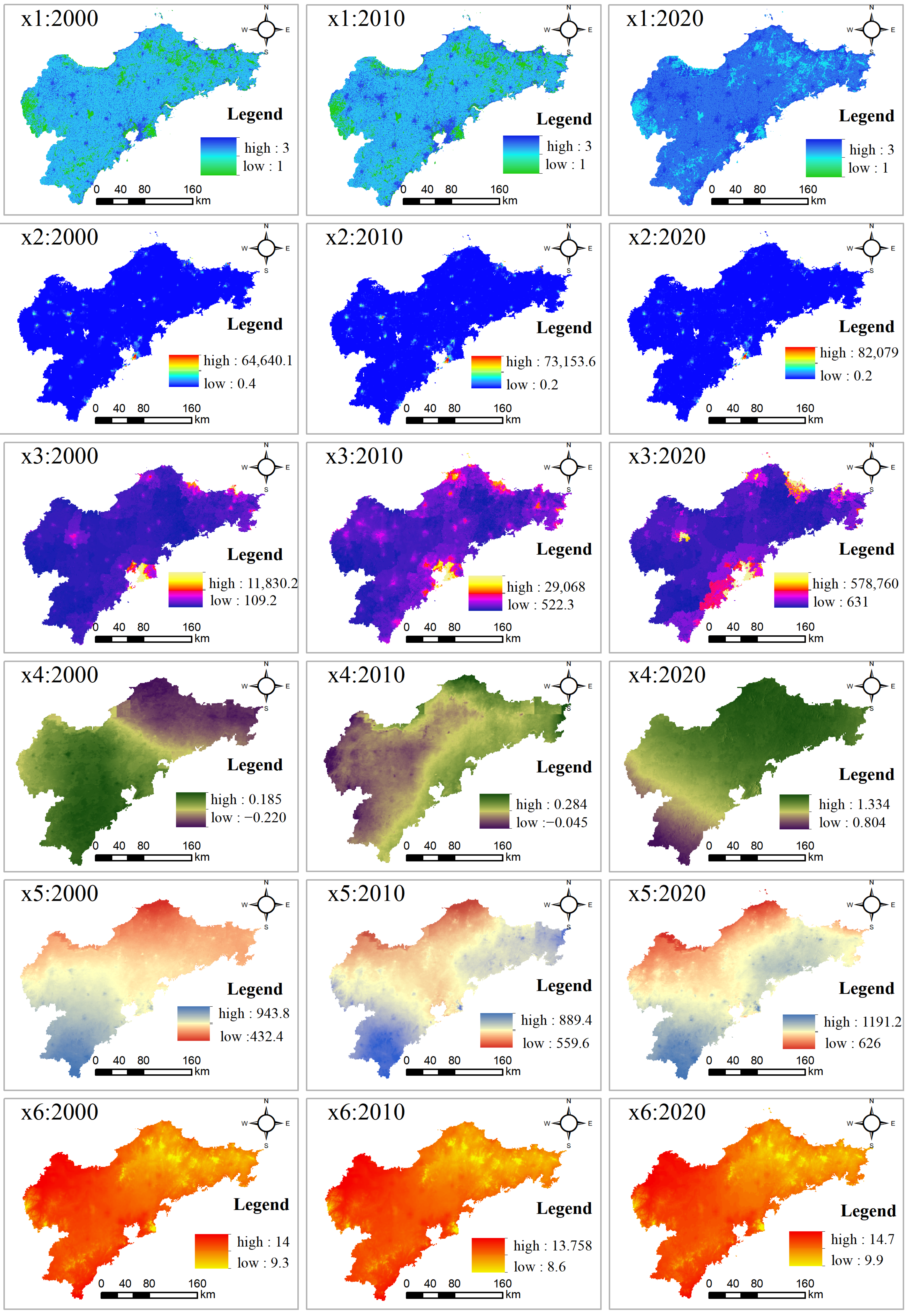
Human activities and natural factors collectively impact EEQ dynamics [40]. The significance of human activities [41,42,43] and natural factors [44,45,46,47] for EEQ varies notably across different research scales. Anchored in the natural environment and socio-economic context of the Jiaodong Peninsula, we identify six driving factors as independent variables, using RSEI as the dependent variable to explore the driving mechanisms (

Table 4. Driving factors for RSEI.

Factor Type	Indicator	Factor Name	Description	Raw Data (Table 2)	Calculation
Human	X1	LUCI	The Land Use Intensity Composite Index reflects the extent of human development and utilization of land in a region, serving as a crucial indicator for measuring both the depth and breadth of land use within an area.	Land Cover	The methodology followed the research of Lili Pu et al. [48] and the weights of land use categories are listed in Table 5.
Human	X2	PD	Population Density reflects the population aggregation situation.	Population Density
Human	X3	GDP	Gross Domestic Product reflects socio-economic activities.	Gross Domestic Product
Nature	X4	SPEI	The Standardized Precipitation Evapotranspiration Index reflects drought conditions by measuring the difference between precipitation and potential evapotranspiration.	Precipitation, Evaporation	The methodology was referenced from the study conducted by Vicente-Serrano et al. [49].
Nature	X5	AMP	Annual Mean Precipitation reflects the impact of precipitation in climate change.	Precipitation
Nature	X6	AMT	Annual Mean Temperature reflects the impact of temperature in climate change.	Temperature

). Considering spatial heterogeneity, data compatibility, and computational sample sizes, all data are resampled to a resolution of 5 km. Figure 2 illustrates the distribution of each driving factor.

2.3.5. RANSAC

Because of the differences in resolution and quality among remote sensing images from different years and sensors, the constructed RSEI image and the images of driving factors inevitably contain noisy data. Directly using linear regression in correlation analysis may lead to significant errors. To explore the relationship between RSEI and the six factors more accurately, this study employs the RANSAC algorithm to calculate the correlation between driving factors and RSEI, and compares with Ordinary Least Squares (OLS).

The RANSAC algorithm is a classic method for fitting models, used to estimate mathematical model parameters from data containing noisy data. Currently, there are no applications of the RANSAC algorithm in the field of ecological assessment. The solving process of the RANSAC algorithm is as follows:

(1)

First, randomly select a set of inlier points from the dataset (the number of which should ensure that all model parameters can be estimated) and calculate a set of model parameters.

(2)

Use the obtained model to test all the other data points. If a point’s error falls within the specified error threshold, it is considered an inlier point; otherwise, it is considered an outlier. Keep only the model with the highest number of inlier points up to this point and record it as the best model.

(3)

Repeat steps 1 and 2 for a sufficient number of times (i.e., reaching the preset iteration limit). Assuming the inlier rate in the dataset is w, the minimum number of iterations k required to obtain a set of inlier points with at least one common inlier at a certain confidence level z is determined by the formula:

$$k=\frac{log(1-z)}{log(1-w^n)},$$

(12)

Use RANSACRegressor function from the scikit-learn library (version 4.1.2) in Python 3.11 to perform inlier–outlier estimation with parameters “loss=squared_error, min_samples=1000”.

2.3.6. GeoDetector

The GeoDetector is a comprehensive tool for revealing the correlation and variation patterns between dependent and independent factors in spatial data. In this study, the dependent factor is RSEI and the independent factors consist of six driving factors. The driving factors are reclassified into five categories of equal frequency.

The GeoDetector includes four modules: the factor detector, risk detector, interaction detector, and ecological detector. The factor detector assesses the influence strength of driving factors on EEQ, while the interaction detector explores the combined effect of any two factors on EEQ.

In the factor detector, a higher q-value indicates a stronger impact of the driving factor on RSEI. The calculation formula for the q-value is

$$q=1-\frac{1}{N{\delta }^2}\sum _{h=1}^L{N}_h{\delta }_h^2,$$

(13)

where $h=1,\dots ,L$; L represents the number of categories for the driving factor; $N_h$ and N denote the sample sizes in different categories and the entire region, respectively; ${\delta }_h^2$ and ${\delta }^2$ represent the variances of RSEI in different categories and the entire region, respectively.

The interaction between two factors can be identified by comparing the q-values of single and double factors. The results of factor interaction detection are classified into 5 categories based on the magnitudes of the q-values for single and double factors (

Table 6. Factor interaction detection results.

Interaction	Judgemental Model
Nonlinear deceleration	$q(X_1\cap X_2)<min(q\left(X_1\right),q\left(X_2\right))$
Linear deceleration	$min(q\left(X_1\right),q\left(X_2\right))<q(X_1\cap X_2)<max(q\left(X_1\right),q\left(X_2\right))$
Bilinear enhancement	$q(X_1\cap X_2)>max(q\left(X_1\right),q\left(X_2\right))$
Mutually independent	$q(X_1\cap X_2)=(q\left(X_1\right)+q\left(X_2\right))$
Nonlinear enhancement	$q(X_1\cap X_2)>(q\left(X_1\right)+q\left(X_2\right))$

).

3. Results

3.1. Spatial and Temporal Evolution of RSEI

Figure 3 illustrates the distribution and proportional areas of RSEI levels across the Jiaodong Peninsula. In 2000, the average RSEI value was 0.60. By 2010, it decreased to 0.57, indicating a 5% decline. However, by 2020, the average RSEI value had risen to 0.66, representing a notable increase of 15.79%. Over the years 2000, 2010, and 2020, areas classified as “Good” and “Excellent” predominated, with proportions of 56.48%, 51.02%, and 67.17%. The proportion of areas classified as “Moderate” increased in 2010 but decreased below the 2000 level by 2020. Conversely, the proportions of “Worst” and “Poor” levels decreased annually, comprising 26.43%, 23.79%, and 19.31% of the total area.

From 2000 to 2010, regions experiencing a strong improvement in RSEI were primarily concentrated in the eastern hilly areas of the Jiaodong Peninsula, while areas exhibiting serious degradation were mainly observed in Weifang and Qingdao. From 2010 to 2020, regions showing a strong improvement in RSEI were predominantly distributed in the eastern hilly areas of the Jiaodong Peninsula, with fewer areas demonstrating serious degradation, which were scattered.

Using the standard deviation ellipse and centroid migration analysis method, this study investigates the spatial distribution characteristics of different levels of RSEI across the Jiaodong Peninsula (Figure 4). The major axis of the standard deviation ellipse indicates the primary direction of RSEI distribution across various levels, while the minor axis signifies the extent of RSEI distribution. The distribution direction of each level of RSEI is consistent, trending from southwest to northeast. For the Good and Excellent levels, the major axis elongates and the minor axis shortens, with the centroid shifting towards the northeast. For the Moderate level, the sizes of the major and minor axes of the standard deviation ellipse remain stable, with minimal changes in the centroid position. For the Worst and Poor levels, the major axis of the standard deviation ellipse shortens, the minor axis widens, and the centroid shifts towards the southwest.

At the urban scale, the rankings of average RSEI values in 2000 were as follows: Rizhao > Weifang > Qingdao > Yantai > Weihai. In 2010, the rankings were: Rizhao > Weifang > Qingdao > Yantai > Weihai. By 2020, the rankings changed to: Rizhao > Weihai > Yantai > Qingdao > Weifang.

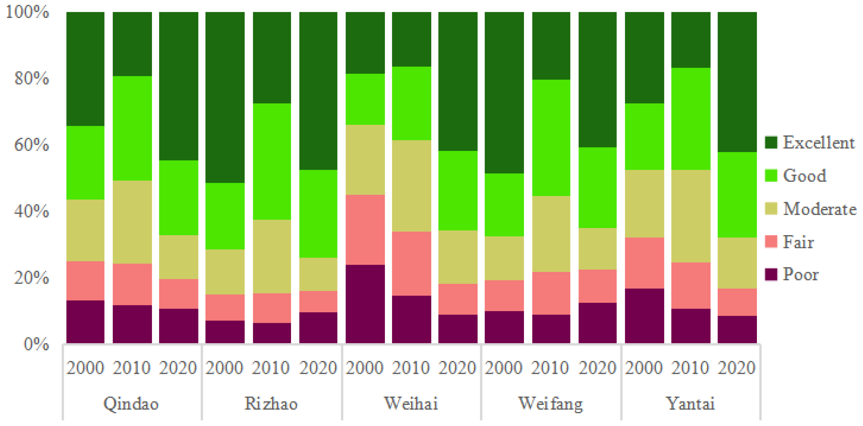
Figure 5 illustrates the proportional distribution of RSEI levels across the five cities of the Jiaodong Peninsula urban agglomeration. The proportions of Good and Excellent areas increased to over 65% in each city, with Rizhao notably reaching 73.85% by 2020. The Moderate areas witnessed an increase in all cities by 2010 followed by a subsequent reduction by 2020. Except for Weifang, the proportions of the Worst and Poor areas reached their lowest levels by 2020.

3.2. Spatial Disparity Analysis of RSEI

The LISA cluster map of RSEI is shown in Figure 6.

2000: H-H clustering areas are primarily located in the mountainous and hilly regions of Rizhao and Weifang cities in the western part of the Jiaodong Peninsula, as well as the Mount Lao district of Qingdao. L-L cluster areas are concentrated in the coastal urban areas and bay regions of each city, with significant L-L clustering also observed in the mountainous and hilly areas of the western part of the Jiaodong Peninsula, especially in Weihai city.

2010: H-H cluster areas remained prominent in the mountainous and hilly terrains of Rizhao and Weifang cities, as well as in the Mount Lao district of Qingdao, albeit with a noticeable decrease in spatial extent. L-L cluster areas continued to appear along the coastal urban zones of each city, although their overall coverage decreased. Notably, clustering within the urban precincts of Weifang and Qingdao expanded during this period, contrasting with the general trend. Other regions did not exhibit significant clustering tendencies.

2020: H-H cluster areas were predominantly distributed in hilly terrains, while the coverage of L-L cluster areas along the coastline notably diminished in Weihai and Yantai cities. L-L cluster areas primarily in the urban zones of Qingdao, Weifang, and the bays of Jiaozhou and Laizhou. The majority of remaining regions did not exhibit pronounced clustering patterns.

3.3. Single-Factor Correlation Analysis Based on RANSAC

In Figure 7, the black and red lines represent the results of least squares (OLS) and RANSAC fitting, respectively. The gray points in the figure denote the inliers fitted by the RANSAC algorithm, while the blue points represent the corresponding outliers or noise points. The coefficient of determination ($R^2$) is used to assess the fitting performance of the algorithms. The $R^2$ values of the RANSAC algorithm consistently exceed those of the OLS method, suggesting the superior capability of the RANSAC algorithm in capturing the influence of factors on the evolution of RSEI.

RANSAC analysis reveal a negative correlation between human activities and RSEI, while the association between natural factors and RSEI demonstrates interannual variations.

The negative correlation between LUCI and RSEI reached its lowest point in 2000 but increased annually thereafter. By 2020, it reached a peak with an R² value of 0.56, the highest among all impact factors.

The $R^2$ for PD and RSEI was relatively low in 2000, reaching its peak in 2010 at 0.25. By 2020, the $R^2$ value for POP ranked second among all impact factors. The negative impact of population aggregation and urbanization on EEQ has become increasingly apparent.

The correlation between GDP and RSEI peaked in 2010. In contrast, the correlation between GDP and RSEI weakened in 2020 compared to PD.

In 2000, SPEI exhibited a positive correlation with RSEI, highlighting the importance of agricultural drought on EEQ. However, this correlation turned negative by 2010 and became inconspicuous by 2020.

AMP exhibits a positive correlation with RSEI, with its $R^2$ value in 2000 only slightly lower than that of SPEI. However, by 2010, the correlation between AMP and RSEI was relatively low. In 2020, the $R^2$ of AMP reached the highest level among the natural factors.

In 2000, there was a positive correlation between AMT and RSEI, although with a low level of correlation. In 2010 and 2020, AMT showed no significant correlation with RSEI.

3.4. Driving Force Analysis Based on GeoDetector

Table 7. q statistic result of GeoDetector.

	2000			2010			2020
Factor	q	p	q Ranking	q	p	q Ranking	q	p	q Ranking
$X_1$	0.048	0.000	5	0.191	0.000	1	0.450	0.000	1
$X_2$	0.037	0.000	6	0.095	0.000	4	0.232	0.000	2
$X_3$	0.168	0.000	4	0.179	0.000	2	0.104	0.000	3
$X_4$	0.222	0.000	1	0.161	0.000	3	0.033	0.000	6
$X_5$	0.189	0.000	2	0.033	0.000	6	0.063	0.000	5
$X_6$	0.170	0.000	3	0.088	0.000	5	0.069	0.000	4

displays the statistical results of GeoDetector’s factor detector.

2000: Natural factors have a greater impact on RSEI compared to human activities. SPEI ranks higher than AMP, with AMT following as the third most influential factor.

2010: Human activities exert a stronger influence on RSEI than natural factors. LUCI had the strongest influence on RSEI evolution. GDP and SPEI are ranked second and third in terms of their importance to RSEI.

2020: Human activity factors dominate the top three spots in the ranking of factor importance. The q-value of LUCI reaching 0.45, with POP’s importance surpassing that of GDP.

The interaction detector results exhibited double-factor and nonlinear enhancement among driving factors (Figure 8).

2000: The SPEI∩GDP interaction, followed by AMP∩GDP, had the greatest impact on EEQ, with a q value reaching 0.358.

2010: The LUCI∩SPEI interaction, followed by LUCI∩AMT, had the greatest impact on EEQ, with a q value reaching 0.383.

2020: The LUCI∩GDP interaction, followed by LUCI∩AMT, had the greatest impact on EEQ, with a q value reaching 0.494.

The double-factor and nonlinear enhancement among human factors gradually intensified, reaching its peak in 2020, while, among nature factors, it decreased annually in 2000, 2010, and 2020.

4. Discussion

4.1. Impact of Natural Factors on EEQ

According to previous studies, the impacts of human activities and natural factors on ecosystems exhibit significant spatial variations [50,51]. In 2000, natural factors outweighed human activity factors in influencing EEQ; SPEI was the predominant determinant of EEQ in the Jiaodong Peninsula (Table 7). The results of the correlation analysis showed that, as SPEI values rise, indicative of alleviation of agricultural drought conditions, RSEI will correspondingly increase (Figure 8).

During 1999–2000, northern China experienced extreme drought disaster due to anomalous circulation over the Eurasian continent [52,53]. During this period, the SPEI values were at their lowest in the eastern Jiaodong Peninsula, indicating the most severe drought conditions. This inhibited vegetation growth and resulted in a significant decline in NDVI, which contributed the most to RSEI (Figure 2 and Table 3). In 2010 and 2020, no extreme drought events occurred, leading to a notable enhancement in EEQ within the eastern hilly regions (Figure 3 and Figure 4). It should be noticed that the importance of SPEI exhibited a gradual decline in 2010 and 2020 compared to 2000 (Figure 8 and Table 7), potentially attributed to advancements in agricultural management practices, including irrigation technology. Hossain et al. [54] propose that, due to disparities in plant drought resilience and agricultural management practices like irrigation, mild drought may not necessarily elicit significant impacts on the ecological environment, indicating that positive human activities can counteract the negative impacts of natural factors. Hua et al. [55] observed that, even in areas with the same land cover type, the eastern regions exhibit higher sensitivity of vegetation activity to drought compared to western regions due to differences in climate and hydrological characteristics. This explains the concentration of L-L cluster areas of RSEI in the eastern regions of the Jiaodong Peninsula in 2000 (Figure 3 and Figure 5).

Compare to SPEI, the importance of AMP and AMT is relatively minor (Table 7), This could be attributed to moderate precipitation and temperature changes, which may not significantly affect enzyme activity within plant tissues. Vegetation exhibits significant decline only when conditions exceed their adaptive range [56,57]. Interaction detection results indicate significant enhancement effects for SPEI∩AMT and AMP∩AMT (Figure 8). Prolonged drought leads to insufficient soil moisture replenishment and exacerbated transpiration due to high temperatures, both of which have detrimental effects on the ecological environment.

With global warming, studies suggest an increased frequency of extreme weather events in the Jiaodong Peninsula [58]. Extreme droughts, floods, frosts, and other natural disasters can lead to reduced vegetation coverage, decreased crop yields, and other ecological issues [59]. Governments should pay attention to enhancing climate event monitoring and warning capabilities, controlling greenhouse gas emissions, and building infrastructure to address climate change. These efforts are necessary to improve climate disaster management and respond promptly to potential ecological risks.

4.2. Impact of Human Activities on EEQ

With the development of the social economy, the impact of human activities on EEQ has gradually increased. In 2010, with favorable natural conditions, the EEQ of the Jiodong Peninsula reached 0.57 (Figure 3). L-L cluster areas were primarily in the urban zones of cities and the coastal zone (Figure 6). LUCI, followed by GDP, became the most significant influencing factor (Table 7). Industrialization and urbanization led to excessive population concentration in cities, resulting in a reduction in per capita natural and social resources, creating immense pressure on the ecological environment of the Jiaodong Peninsula, and even brought about higher risks to life safety [60].

With the increasing awareness of sustainable development and the growing need for a better urban living environment, Shandong Province and the five cities of Jiaodong Peninsula have formulated a series of targeted ecological protection policies over the past 20 years. By 2020, with favorable natural conditions, the EEQ of the Jiaodong Peninsula had increased to 0.67. However, in the urban zones of Weifang City and coastal ecological sources such as Jiaozhou Bay, the L-L cluster areas continued to increase (Figure 6). The interaction effect of land use with other driving factors reached its peak in 2020 (Figure 8).

To mitigate the negative effects of human activities on the complex coastal ecosystem of the Jiaodong Peninsula, we propose the following recommendations: (1) In urban zones where L-L cluster areas are mainly concentrated, human activities should be regulated and more green spaces should be planned within the cities to control the expansion of urban areas. (2) In hilly regions, human intervention should be reduced to maintain the integrity of natural landscapes and protect natural resources such as forests and farmland. Attention should be paid to natural restoration in important natural reserves or ecological sources like Lao Mountain, and artificial intervention methods such as cloud seeding can be employed if necessary. (3) In important coastal areas like Jiaozhou Bay and Laizhou Bay, strict regulations should be imposed on excessive development activities such as artificial land reclamation. More ecological enhancement projects such as increasing the area of wetland parks should be implemented. (4) Balancing urban and rural development and providing fair access to education and healthcare are effective in easing urban population pressure.

4.3. Limitations and Prospects

Compared to single-factor analysis, RSEI can provide richer information on the ecological environment. However, RSEI is only applicable to terrestrial areas, and indicators such as the distribution of water resources and environmental pollution cannot be incorporated into the assessment method, indicating a need to enrich the dimensions of RSEI. In future research, we should consider incorporating carbon emissions and environmental pollution factors into the assessment system to construct a more comprehensive ecological remote sensing assessment method.

This research using Landsat data with a spatial resolution of 30 m for the years 2000, 2010, and 2020. Therefore, we are unable to provide the nuanced changes over a twenty-year period of EEQ. Due to challenges in obtaining annual data on land cover and GDP, we were unable to investigate the temporal lagged effects of driving factors at a consistent temporal resolution. In the future, with improved data availability, we will consider extending the research to include historical data or future projections.

5. Conclusions

This study utilized RSEI to evaluate EEQ and employed standard deviation ellipses, centroid migration, and LISA clustering methods to assess the spatiotemporal distribution changes and spatial clustering effects of EEQ in the Jiaodong Peninsula for the years 2000, 2010, and 2020. To mitigate noise interference in remote sensing images, we applied the RANSAC algorithm, resulting in single-factor correlations between human and natural factors and RSEI. Additionally, GeoDetector was utilized to quantify the contributions of human and natural factors to EEQ and their interactions during the same years.

The results indicate that the Jiaodong Peninsula generally exhibits favorable EEQ, with average RSEI values of 0.60, 0.57, and 0.65 for 2000, 2010, and 2020, with Good and Excellent level areas comprising the largest proportion. For Good and Excellent RSEI levels, the centroid shifted towards the northeast. The cluster map of RSEI revealed that H-H cluster areas were primarily located in hilly regions, while L-L cluster areas were mainly found in urban and coastal areas around Laizhou Bay and Jiaozhou Bay.

The driving analysis results revealed that, in 2000, the significance of nature factors exceeded that of human factors. SPEI emerged as the predominant determinant of EEQ, with a q value reaching 0.222. However, in 2010 and 2020, the negative effects of human factors gradually intensified, with LUCI identified as the most influential driving factor, having q values of 0.191 and 0.450. The driving factors exhibited double-factor and nonlinear enhancement. The most significant interaction factors affecting the EEQ of the Jiaodong Peninsula in 2000, 2010, and 2020 were identified as SPEI∩GDP, LUCI∩SPEI, and LUCI∩GDP.

Governments and environmental protection agencies should implement measures such as improving climate disaster management, increasing urban green space planning, strengthening coastal ecological enhancement projects, and protecting critical ecological sources to enhance the resilience of the complex coastal ecosystem, promoting the sustainable development of the Jiaodong Peninsula.

References

- Findell, K.L.; Berg, A.; Gentine, P.; Krasting, J.P.; Lintner, B.R.; Malyshev, S.; Santanello, J.A., Jr.; Shevliakova, E. The impact of anthropogenic land use and land cover change on regional climate extremes. Nat. Commun. 2017, 8, 989. [Google Scholar] [CrossRef] [PubMed]
- Frate, L.; Carranza, M.L.; Evangelista, A.; Stinca, A.; Schaminée, J.H.; Stanisci, A. Climate and land use change impacts on Mediterranean high-mountain vegetation in the Apennines since the 1950s. Plant Ecol. Divers. 2018, 11, 85–96. [Google Scholar] [CrossRef]
- Bejagam, V.; Sharma, A. Impact of climatic changes and anthropogenic activities on ecosystem net primary productivity in India during 2001–2019. Ecol. Inform. 2022, 70, 101732. [Google Scholar] [CrossRef]
- Weiskopf, S.R.; Rubenstein, M.A.; Crozier, L.G.; Gaichas, S.; Griffis, R.; Halofsky, J.E.; Hyde, K.J.; Morelli, T.L.; Morisette, J.T.; Muñoz, R.C.; et al. Climate change effects on biodiversity, ecosystems, ecosystem services, and natural resource management in the United States. Sci. Total. Environ. 2020, 733, 137782. [Google Scholar] [CrossRef] [PubMed]
- Torres, A.V.; Tiwari, C.; Atkinson, S.F. Progress in ecosystem services research: A guide for scholars and practitioners. Ecosyst. Serv. 2021, 49, 101267. [Google Scholar] [CrossRef]
- Dossou, J.F.; Li, X.; Sadek, M.; Almouctar, M.A.S.; Mostafa, E. Hybrid model for ecological vulnerability assessment in Benin. Sci. Rep. 2021, 11, 2449. [Google Scholar] [CrossRef] [PubMed]
- Ding, M.J.; Liu, W.Q.; Xiao, L.; Zhong, F.; Lu, N.; Zhang, J.; Zhang, Z.Q.; Xu, X.; Wang, K. Construction and optimization strategy of ecological security pattern in a rapidly urbanizing region: A case study in central-south China. Ecol. Indic. 2022, 136, 108604. [Google Scholar] [CrossRef]
- Świąder, M.; Lin, D.; Szewrański, S.; Kazak, J.K.; Iha, K.; van Hoof, J.; Belčáková, I.; Altiok, S. The application of ecological footprint and biocapacity for environmental carrying capacity assessment: A new approach for European cities. Environ. Sci. Policy 2020, 105, 56–74. [Google Scholar] [CrossRef]
- Xu, H. A remote sensing urban ecological index and its application. Acta Ecol. Sin 2013, 33, 7853–7862. [Google Scholar]
- Martinez, A.; Labib, S.M. Demystifying normalized difference vegetation index (NDVI) for greenness exposure assessments and policy interventions in urban greening. Environ. Res. 2022, 220, 115155. [Google Scholar] [CrossRef] [PubMed]
- Amin, E.; Verrelst, J.; Rivera-Caicedo, J.P.; Pipia, L.; Ruiz-Verdú, A.; Moreno, J.F. Prototyping Sentinel-2 green LAI and brown LAI products for cropland monitoring. Remote Sens. Environ. 2020, 255, 112168. [Google Scholar] [CrossRef] [PubMed]
- Saleh, S.K.; Amoushahi, S.; Gholipour, M. Spatiotemporal ecological quality assessment of metropolitan cities: A case study of central Iran. Environ. Monit. Assess. 2021, 193, 305. [Google Scholar] [CrossRef] [PubMed]
- Chen, N.; Cheng, G.; Yang, J.; Ding, H.; He, S. Evaluation of Urban Ecological Environment Quality Based on Improved RSEI and Driving Factors Analysis. Sustainability 2023, 15, 8464. [Google Scholar] [CrossRef]
- Cao, J.Z.; Wu, E.; Wu, S.; Fan, R.; Xu, L.; Ning, K.; Li, Y.; Lu, R.C.; Xu, X.; Zhang, J.; et al. Spatiotemporal Dynamics of Ecological Condition in Qinghai-Tibet Plateau Based on Remotely Sensed Ecological Index. Remote Sens. 2022, 14, 4234. [Google Scholar] [CrossRef]
- Wang, H.; Liu, C.; Zang, F.; Liu, Y.; Chang, Y.; Huang, G.; Fu, G.; Zhao, C.; Liu, X. Remote Sensing-Based Approach for the Assessing of Ecological Environmental Quality Variations Using Google Earth Engine: A Case Study in the Qilian Mountains, Northwest China. Remote Sens. 2023, 15, 960. [Google Scholar] [CrossRef]
- An, M.W.; Xie, P.; He, W.; Wang, B.B.; Huang, J.; Khanal, R. Spatiotemporal change of ecologic environment quality and human interaction factors in three gorges ecologic economic corridor, based on RSEI. Ecol. Indic. 2022, 141, 109090. [Google Scholar] [CrossRef]
- Qiu, S.; Zhu, Z.; Olofsson, P.; Woodcock, C.E.; Jin, S. Evaluation of Landsat image compositing algorithms. Remote Sens. Environ. 2023, 285, 113375. [Google Scholar] [CrossRef]
- Ajayi, O.G.; Ojima, A. Performance evaluation of selected cloud occlusion removal algorithms on remote sensing imagery. Remote Sens. Appl. Soc. Environ. 2022, 25, 100700. [Google Scholar] [CrossRef]
- Kowarik, I. Urban biodiversity, ecosystems and the city. Insights from 50 years of the Berlin School of urban ecology. Landsc. Urban Plan. 2023, 240, 104877. [Google Scholar] [CrossRef]
- Cai, F.; Cao, C.; Qi, H.; Su, X.; Lei, G.; Liu, J.; Zhao, S.; Liu, G.; Zhu, K. Rapid migration of mainland China’s coastal erosion vulnerability due to anthropogenic changes. J. Environ. Manag. 2022, 319, 115632. [Google Scholar] [CrossRef] [PubMed]
- Yan, Y.; Ju, H.; Zhang, S.; Chen, G. The construction of ecological security patterns in coastal areas based on landscape ecological risk assessment—A case study of Jiaodong Peninsula, China. Int. J. Environ. Res. Public Health 2021, 18, 12249. [Google Scholar] [CrossRef] [PubMed]
- Huang, L.; Wang, J.; Cheng, H. Spatiotemporal changes in ecological network resilience in the Shandong Peninsula urban agglomeration. J. Clean. Prod. 2022, 339, 130681. [Google Scholar] [CrossRef]
- Kang, J.; Zhang, X.; Zhu, X.; Zhang, B. Ecological security pattern: A new idea for balancing regional development and ecological protection. A case study of the Jiaodong Peninsula, China. Glob. Ecol. Conserv. 2021, 26, e01472. [Google Scholar] [CrossRef]
- Yu, L.; Wu, X.; Zheng, X.; Zheng, T.; Xin, J.; Walther, M. An index system constructed for ecological stress assessment of the coastal zone: A case study of Shandong, China. J. Environ. Manag. 2019, 232, 499–504. [Google Scholar] [CrossRef] [PubMed]
- Zuo, D.; Cai, S.; Xu, Z.; Li, F.; Sun, W.; Yang, X.; Kan, G.; Liu, P.Y. Spatiotemporal patterns of drought at various time scales in Shandong Province of Eastern China. Theor. Appl. Climatol. 2016, 131, 271–284. [Google Scholar] [CrossRef]
- Fischler, M.A.; Bolles, R.C. Random sample consensus: A paradigm for model fitting with applications to image analysis and automated cartography. Commun. ACM 1981, 24, 381–395. [Google Scholar] [CrossRef]
- Salehi, B.; Jarahizadeh, S.; Sarafraz, A. An Improved RANSAC Outlier Rejection Method for UAV-Derived Point Cloud. Remote Sens. 2022, 14, 4917. [Google Scholar] [CrossRef]
- Wang, J.; Xu, C. Geodetector: Principle and prospective. Acta Geogr. Sin 2017, 72, 116–134. [Google Scholar]
- Peng, Q.; Wang, R.; Jiang, Y.; Zhang, W.; Liu, C.; Zhou, L. Soil erosion in Qilian Mountain National Park: Dynamics and driving mechanisms. J. Hydrol. Reg. Stud. 2022, 42, 101144. [Google Scholar] [CrossRef]
- He, J.; Pan, Z.; Liu, D.; Guo, X. Exploring the regional differences of ecosystem health and its driving factors in China. Sci. Total. Environ. 2019, 673, 553–564. [Google Scholar] [CrossRef] [PubMed]
- Xu, H.; Deng, W. Rationality analysis of MRSEI and its difference with RSEI. Remote Sens. Technol. Appl. 2022, 37, 1–7. [Google Scholar]
- Crist, E.P. A TM tasseled cap equivalent transformation for reflectance factor data. Remote Sens. Environ. 1985, 17, 301–306. [Google Scholar] [CrossRef]
- Baig, M.H.A.; Zhang, L.; Shuai, T.; Tong, Q. Derivation of a tasselled cap transformation based on Landsat 8 at-satellite reflectance. Remote Sens. Lett. 2014, 5, 423–431. [Google Scholar] [CrossRef]
- Gao, W.; Zhang, S.; Rao, X.; Lin, X.; Li, R. Landsat TM/OLI-based ecological and environmental quality survey of Yellow River Basin, Inner Mongolia Section. Remote Sens. 2021, 13, 4477. [Google Scholar] [CrossRef]
- Xu, H.; Wang, M.; Shi, T.; Guan, H.; Fang, C.; Lin, Z. Prediction of ecological effects of potential population and impervious surface increases using a remote sensing based ecological index (RSEI). Ecol. Indic. 2018, 93, 730–740. [Google Scholar] [CrossRef]
- Xiong, Y.; Xu, W.; Lu, N.; Huang, S.; Wu, C.; Wang, L.; Dai, F.; Kou, W. Assessment of spatial–temporal changes of ecological environment quality based on RSEI and GEE: A case study in Erhai Lake Basin, Yunnan province, China. Ecol. Indic. 2021, 125, 107518. [Google Scholar] [CrossRef]
- Li, Z.L.; Wu, H.; Duan, S.B.; Zhao, W.; Ren, H.; Liu, X.; Leng, P.; Tang, R.; Ye, X.; Zhu, J.; et al. Satellite remote sensing of global land surface temperature: Definition, methods, products, and applications. Rev. Geophys. 2023, 61, e2022RG000777. [Google Scholar] [CrossRef]
- Zhang, X.; Jia, W.; He, J. Spatial and temporal variation of ecological quality in northeastern China and analysis of influencing factors. J. Clean. Prod. 2023, 423, 138650. [Google Scholar] [CrossRef]
- Zhang, L.; Jia, X.; Zhao, Y.; Wang, H.; Peng, B.; Zhang, P.; Zhao, M. Spatio-temporal characteristics and driving mechanism of land degradation sensitivity in Northwest China. Sci. Total. Environ. 2024, 918, 170403. [Google Scholar] [CrossRef] [PubMed]
- Zeng, J.; Dai, X.; Li, W.; Xu, J.; Li, W.; Liu, D. Quantifying the Impact and Importance of Natural, Economic, and Mining Activities on Environmental Quality Using the PIE-Engine Cloud Platform: A Case Study of Seven Typical Mining Cities in China. Sustainability 2024, 16, 1447. [Google Scholar] [CrossRef]
- Sui, Y.; Hu, J.; Zhang, N.; Ma, F. Exploring the dynamic equilibrium relationship between urbanization and ecological environment—A case study of Shandong Province, China. Ecol. Indic. 2024, 158, 111456. [Google Scholar] [CrossRef]
- Bai, T.; Cheng, J.; Zheng, Z.; Zhang, Q.; Li, Z.; Xu, D. Drivers of eco-environmental quality in China from 2000 to 2017. J. Clean. Prod. 2023, 396, 136408. [Google Scholar] [CrossRef]
- Basu, T.; Das, A. Systematic review of how eco-environmental transformation due to urbanization can be investigated in the sustainable development of Indian cities. Environ. Chall. 2021, 4, 100099. [Google Scholar] [CrossRef]
- Alatalo, J.M.; Jägerbrand, A.K.; Dai, J.; Mollazehi, M.D.; Abdel-Salam, A.S.G.; Pandey, R.; Molau, U. Effects of ambient climate and three warming treatments on fruit production in an alpine, subarctic meadow community. Am. J. Bot. 2021, 108, 411–422. [Google Scholar] [CrossRef] [PubMed]
- Zhao, H.; Huang, Y.; Wang, X.; Li, X.; Lei, T. The performance of SPEI integrated remote sensing data for monitoring agricultural drought in the North China Plain. Field Crop. Res. 2023, 302, 109041. [Google Scholar] [CrossRef]
- Feldman, A.F.; Short Gianotti, D.J.; Trigo, I.F.; Salvucci, G.D.; Entekhabi, D. Observed landscape responsiveness to climate forcing. Water Resour. Res. 2022, 58, e2021WR030316. [Google Scholar] [CrossRef]
- Feldman, A.F.; Short Gianotti, D.J.; Dong, J.; Trigo, I.F.; Salvucci, G.D.; Entekhabi, D. Tropical surface temperature response to vegetation cover changes and the role of drylands. Glob. Chang. Biol. 2023, 29, 110–125. [Google Scholar] [CrossRef] [PubMed]
- Pu, L.; Lu, C.; Yang, X.; Chen, X. Spatio-Temporal Variation of the Ecosystem Service Value in Qilian Mountain National Park (Gansu Area) Based on Land Use. Land 2023, 12, 201. [Google Scholar] [CrossRef]
- Vicente-Serrano, S.M.; Beguería, S.; López-Moreno, J.I. A multiscalar drought index sensitive to global warming: The standardized precipitation evapotranspiration index. J. Clim. 2010, 23, 1696–1718. [Google Scholar] [CrossRef]
- Yuan, B.; Fu, L.; Zou, Y.; Zhang, S.; Chen, X.; Li, F.; Deng, Z.; Xie, Y. Spatiotemporal change detection of ecological quality and the associated affecting factors in Dongting Lake Basin, based on RSEI. J. Clean. Prod. 2021, 302, 126995. [Google Scholar] [CrossRef]
- Zhang, X.; Fan, H.; Sun, L.; Liu, W.; Wang, C.; Wu, Z.; Lv, T. Identifying regional eco-environment quality and its influencing factors: A case study of an ecological civilization pilot zone in China. J. Clean. Prod. 2023, 435, 140308. [Google Scholar] [CrossRef]
- Jie, W.; Qingyun, Z.; Shiyan, T. Physical causes of the 1999 and 2000 summer severe drought in North China. Chin. J. Atmos. Sci. Chin. Ed. 2004, 28, 124–137. [Google Scholar]
- Zhang, L.; Xiao, J.; Zhou, Y.; Zheng, Y.; Li, J.; Xiao, H. Drought events and their effects on vegetation productivity in China. Ecosphere 2016, 7, e01591. [Google Scholar] [CrossRef]
- Hossain, M.L.; Li, J. NDVI-based vegetation dynamics and its resistance and resilience to different intensities of climatic events. Glob. Ecol. Conserv. 2021, 30, e01768. [Google Scholar] [CrossRef]
- Hua, T.; Wang, X.; Zhang, C.; Lang, L.; Li, H. Responses of vegetation activity to drought in northern China. Land Degrad. Dev. 2017, 28, 1913–1921. [Google Scholar] [CrossRef]
- Akinyemi, D.S.; Zhu, Y.; Zhao, M.; Zhang, P.; Shen, H.; Fang, J. Response of soil extracellular enzyme activity to experimental precipitation in a shrub-encroached grassland in Inner Mongolia. Glob. Ecol. Conserv. 2020, 23, e01175. [Google Scholar] [CrossRef]
- Zeppel, M.; Wilks, J.V.; Lewis, J.D. Impacts of extreme precipitation and seasonal changes in precipitation on plants. Biogeosciences 2014, 11, 3083–3093. [Google Scholar] [CrossRef]
- Wang, H.; Wang, L.; Yan, G.; Bai, H.; Zhao, Y.; Ju, M.; Xu, X.; Yan, J.; Xiao, D.; Chen, L. Assessment and prediction of extreme temperature indices in the North China Plain by CMIP6 climate model. Appl. Sci. 2022, 12, 7201. [Google Scholar] [CrossRef]
- Bai, H.; Xiao, D.; Wang, B.; Liu, D.L.; Feng, P.; Tang, J. Multi-model ensemble of CMIP6 projections for future extreme climate stress on wheat in the North China plain. Int. J. Climatol. 2021, 41, E171–E186. [Google Scholar] [CrossRef]
- Arbel, Y.; Fialkoff, C.; Kerner, A.; Kerner, M. Do population density, socio-economic ranking and Gini Index of cities influence infection rates from coronavirus? Israel as a case study. Ann. Reg. Sci. 2022, 68, 181–206. [Google Scholar] [CrossRef] [PubMed]
Figure 1.
Location of Jiaodong Peninsula.
Figure 2.
Driving factors of RSEI in Jiaodong peninsula. Factor abbreviations are listed in Table 4.
Figure 3.
Spatial distribution of RSEI levels in Jiaodong Peninsula.
Figure 4.
Standard deviation ellipse analysis and centroid migration for different levels of the RSEI.
Figure 5.
The percentage of RSEI levels area in cities from 2000 to 2020.
Figure 6.
LISA cluster map of RSEI.
Figure 7.
RANSAC and OLS fitting results of RSEI. Factor abbreviations are listed in Table 4.
Figure 8.
q values of interaction detector. Factor abbreviations are listed in Table 4.