
Efficiency Analysis of Electric Vehicles with AMT and Dual-Motor Systems
by

Zhenghong Wang
1,2,†, 
Xudong Qu
1,2,†,
Qingling Cai
1,2,
Fulin Chu
2,
Jiaheng Wang
2 and
Dapai Shi
1,2,* 1
Hubei Longzhong Laboratory, Hubei University of Arts and Science, Xiangyang 441000, China
2
Hubei Key Laboratory of Power System Design and Test for Electrical Vehicle, Hubei University of Arts and Science, Xiangyang 441053, China
*
Author to whom correspondence should be addressed.
†
These authors contributed equally to this work.
World Electr. Veh. J. 2024, 15(5), 182; https://doi.org/10.3390/wevj15050182
Submission received: 13 March 2024
/
Revised: 6 April 2024
/
Accepted: 16 April 2024
/
Published: 24 April 2024
Abstract
:With the rapid development of automobiles, energy shortages and environmental pollution have become a growing concern. In order to decrease the energy consumption of electric vehicles (EVs), this study aims to improve EV efficiency with AMT and dual-motor systems. Firstly, the paper establishes an Automated Manual Transmission (AMT) model for EVs, which is then simulated using MATLAB R2022a software. In order to eliminate the impact of gear ratio selection, the genetic algorithm is used to optimize the AMT gear ratios. Meanwhile, a dual-motor EV model is constructed, and three different torque distribution schemes are simulated and analyzed. The results indicate that due to the elongation of the energy transmission chain in AMT-equipped EVs, energy losses increase, leading to some improvement in optimized power consumption. However, these EVs remain inferior to those with only a single-stage main reducer. The study also found that the torque distribution based on optimal efficiency further improves results.
1. Introduction
As the automotive industry progresses rapidly, the use of petroleum has sparked serious concerns regarding environmental pollution and energy shortages. These issues have catalyzed a consensus on the demand for new energy vehicles [1,2]. Electric vehicles (EVs), known for their environmental friendliness, energy efficiency, and reduced dependence on non-renewable energy sources, are considered an optimal solution for future transportation [3]. However, the driving range of EVs is comparatively short due to the limited energy density of batteries, making them primarily suitable for short-distance travel [4]. Therefore, extending their driving range and improving their economic performance is crucial for their widespread adoption. Alcázar-García et al. [5] developed a model utilizing genetic algorithms to maximize vehicle range with minimal effort, while also generating predictive information that can optimize design. This model not only boasts high accuracy, but also demonstrates strong universality and reliability, thereby accelerating advancements in the automotive industry.
The growing number of electric vehicles necessitates an increasing amount of energy for charging their traction batteries. Electric vehicles are most eco-friendly when the energy for charging comes from renewable sources. Caban et al. [6] proposed a strategic model that takes into account the location and climate background of photovoltaic systems, automatically adjusting planning based on energy demand, to utilize photovoltaic system energy for charging electric vehicle fleets. Furthermore, Piotrowska et al. [7] conducted a lifecycle assessment and analysis of wind and photovoltaic power stations across three impact areas—human health, ecosystems, and resources—providing valuable insights into the environmental impacts of renewable energy systems.
As the sole power source for EVs, the drive motor operates over a wide speed range and typically does not require a multi-speed gearbox to meet the vehicle’s maximum speed requirements [8]. The motor is most efficient within its rated speed range [9,10]. For EVs employing a single-stage primary reducer, the operating points of the motor span the entire speed range, leading to a waste of appropriate motor power and, consequently, a negative impact on the economic performance of EVs [11]. Choosing an inappropriate motor power for an EVS can increase costs and reduce travel distance [12]. Thus, research into Automated Manual Transmissions (AMT) for EVs becomes necessary, aiming to optimize their efficiency and further facilitate the adoption of environmentally sustainable transportation solutions.
1.1. Current Research Status of EVs with Automated Manual Transmission
Based on test models, Ruan et al. [13] modeled and simulated EVs with dual AMT, as well as 3-speed and 4-speed AMT. Comparing motor performance and efficiency revealed that EVs with AMTs exhibit higher motor efficiency. Lin et al. [14] demonstrated that improved shifting techniques could enhance the economy and driving performance of 2-speed EVs with AMT. He et al. [15] developed a shifting strategy and controller to improve vehicle efficiency and range, employing a hybrid fuzzy control- and iterative learning control-based shifting rule switch controller. The strategy, considering energy consumption, acceleration, and battery state of charge, achieved its objectives. Shen et al. [16] improved the vehicle’s overall economy by optimizing the gear ratios of a 2-speed AMT. Borthakur et al. [17] used a nondominated sorting genetic algorithm to optimize the gear ratios of a 2-speed EV with AMT, enhancing the vehicle’s economy and driving performance. Ganesan et al. [18] coordinated the shifting process of a 2-speed AMT and achieved precise control of the shifting execution motor using a model predictive control algorithm. Fu et al. [19] formulated a dual-parameter shifting rule for a commercial AMT, taking vehicle speed and motor torque as shifting parameters, achieving an optimal compromise between battery and motor efficiency.
Future research should consider creating a clutchless multi-stage AMT for electric vehicles, which could enhance motor efficiency and extend battery life. The Porsche Taycan is equipped with a single-speed transmission on both the front and rear axles and a dual-speed transmission that enhances efficiency at low and high speeds, improving the vehicle’s range and acceleration capability.
It is evident from these studies that EVs with AMTs exhibit better acceleration, consume less energy, and achieve higher maximum speeds [20]. Additionally, integrating multiple gears into AMTs alleviates the strain on the electric motor, thereby extending its lifespan and adding to the reliability and stability of EVs [21,22].
1.2. Current Research Status of Dual-Motor EVs
Yu et al. [23] developed a four-speed clutchless transmission system for EVs with dual-motor, comparing its performance to single-motor direct-drive and two-gear transmission setups through a simulation model. Tian et al. [24] compared a speed-coupled dual-motor drive structure to a single-motor structure with a reducer, finding that the former significantly enhances vehicle efficiency. Wang et al. [25] used a planetary gear arrangement to achieve dual-motor independent and speed-coupled drive structures. Zhu et al. [26] designed a dual-motor drive system that improves vehicle performance by optimizing driving and braking torque distribution based on operation and load conditions. Hu et al. [27] proposed a torque-adjustable dual-motor drive system based on tire slip rate and driving conditions. Nguyen et al. [28] developed a dual-motor drive system with four modes and optimized power allocation using a sequential quadratic programming algorithm. Wang et al. [29] validated dual-motor transmission system parameters optimized by genetic algorithms through a simulation platform. A real-time control strategy and dynamic mode switching process were tested on benches to confirm effectiveness.
In 2018, Honda released their newest i-MMD system, which included Atkinson engines and powerful dual-motor CVTs. Audi also unveiled their luxurious all-electric SUV, the E-Tron, featuring asynchronous motors on both the front and rear axles, allowing for two- and four-wheel drive modes [30].
Could the economy and performance of the Porsche Taycan be improved by adding more gears to its two-speed transmission or dual-motor configuration? To investigate the effects of additional gears and speed ratios on the performance and efficiency of electric vehicles (EVs), this study modified EVs equipped with a single-stage main reducer by adding two-, three-, and four-speed gearboxes. The experiment revealed that while adding more gears did provide some optimization benefits, the improvements to the vehicle’s economy and power were limited and still not comparable to EVs with only a single-stage main reducer.
Moreover, this study developed a dual-motor drive system model and analyzed three different torque distribution strategies: torque equalization, single-motor priority, and dual-motor priority. On this basis, the motor scaling factor was adjusted in order to examine its impact on the energy consumption of dual-motor EVs. In-depth analysis of the simulation results showed that a motor scaling factor of 0.5 yielded the lowest energy consumption for all three torque distribution strategies. When optimizing the economy of dual-motor EVs, the dual-motor efficiency priority strategy demonstrated the best performance.
1.3. Summary of Article Structure
- ▪
- S1: Introduction
- ▪
- S2: Modeling and Optimization of Automated Manual Transmission and Dual-Motor EVs
- ▪
- S3: Simulation Results and Analysis of EV with Automated Manual Transmission
- ▪
- S4: Conclusions
2. Modeling and Optimization of Automated Manual Transmission and Dual-Motor EVs
2.1. Modeling and Optimization of EV with AMT
2.1.1. Modeling of EV with Automated Manual Transmission
- (1)
- Single-Stage Main Reducer Model Establishment
In order to build the vehicle model, the basic parameters of the vehicle should be obtained, mainly referring to the fundamental dimensional parameters, as shown in Table 1.
- (a)
- Single-stage main reducer EV powertrain architecture.
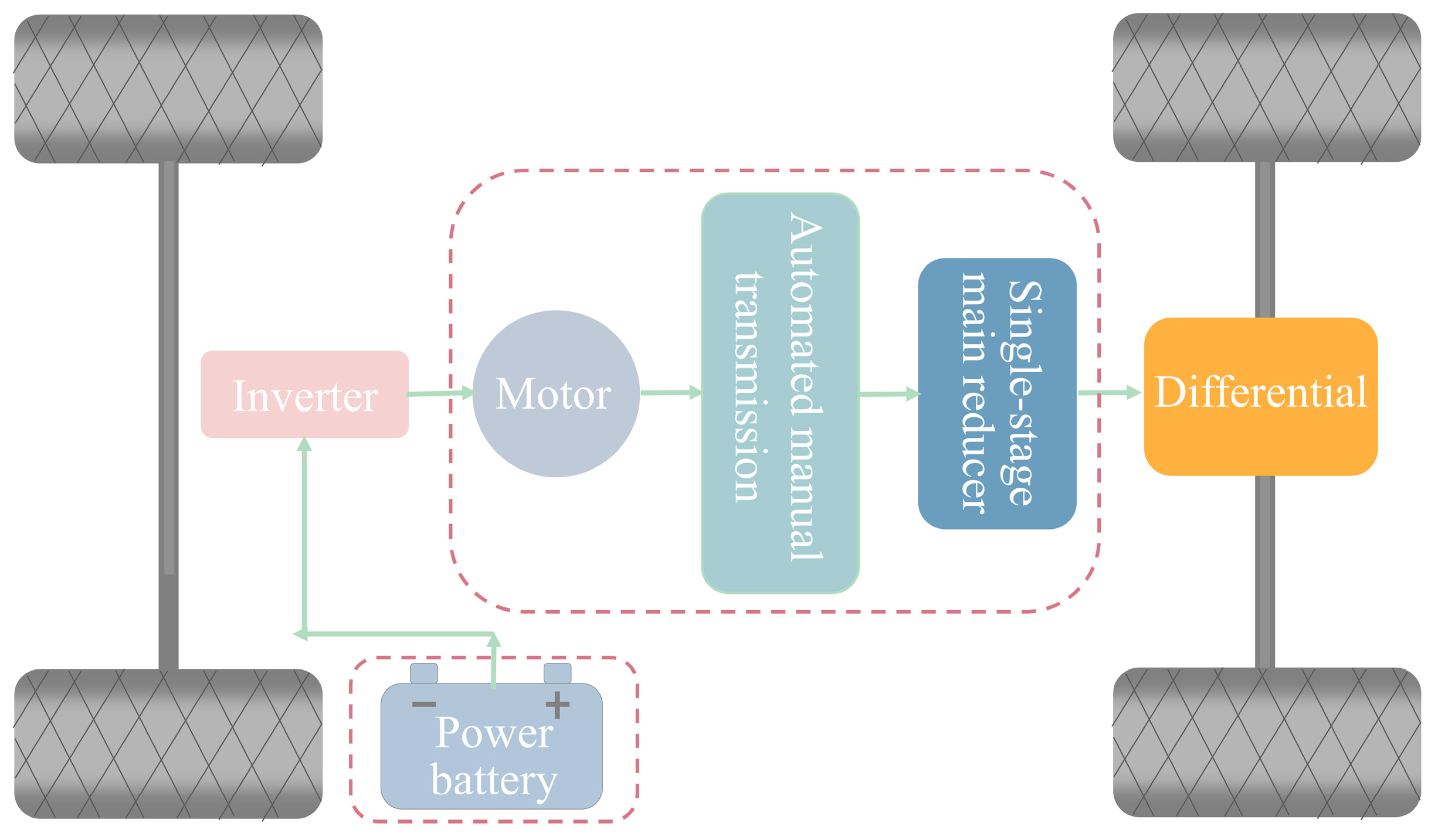
The powertrain architecture employing a single-stage primary reducer, as illustrated in Figure 1, encompasses the power battery, inverter, motor, single-stage primary reducer, and differential. The study subsequently analyzes the energy loss and average efficiency of the components outlined by the red dashed frame.
- (b)
- Motor Modeling
The motor is a crucial component of the pure electric vehicle power system. Its primary function is to convert the electrical energy from the traction battery into mechanical energy for the transmission system, providing sufficient torque to the drive wheels. During daily driving, it transforms braking energy into direct current, storing it in the battery for future use. The motor is modeled using the method based on the static efficiency MAP (Motor Axial Power) chart. The following equation can determine the relationship between motor efficiency and motor speed and torque:
where represents the real-time efficiency of the motor, stands for the motor torque, and represents the motor speed; the constant 9550 is used as a factor to convert torque and rotational speed to power.
In different usage scenarios, the motor operates in different states, which can be categorized into driving mode and charging mode. When the torque is positive, the motor converts electrical energy into mechanical energy, whereas when the torque is negative, it indicates that the vehicle is braking. In this case, the motor converts mechanical energy back into chemical energy to charge the battery. The formulas for calculating motor power in different modes are as follows:
Figure 2 illustrates the variation in torque and power of the motor at different speeds.
- (c)
- Battery Modeling
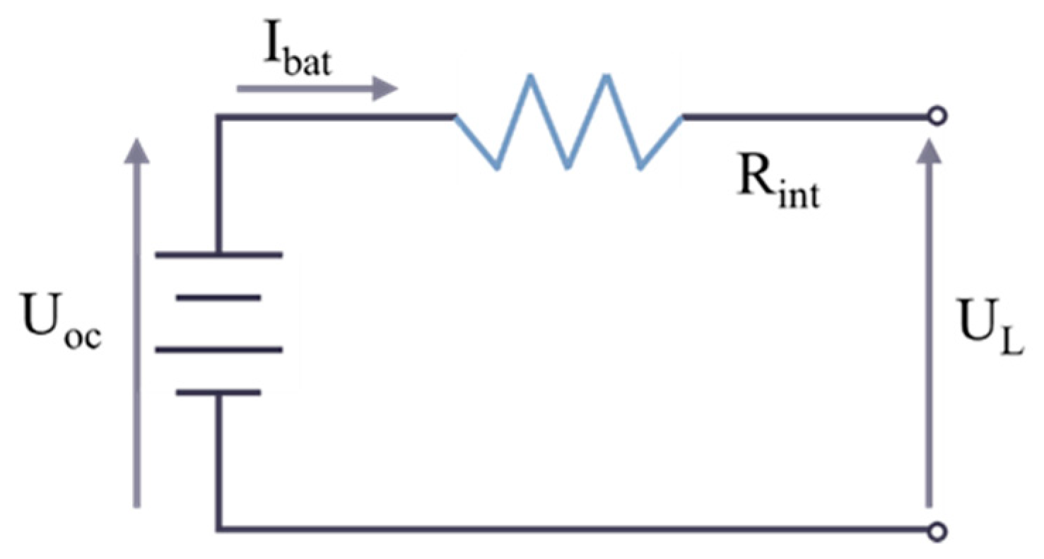
As a crucial device for supplying and storing energy, the traction battery undergoes complex material, chemical, and physical changes during the charging and discharging processes. These changes are nonlinear, making it challenging to establish a theoretical model for the traction battery. Various modeling methods exist for traction batteries, including lookup table methods, first-order RC models, and second-order RC models. In this study, the first-order RC model was chosen for battery modeling, and the schematic diagram is shown in Figure 3.
The equivalent circuit equation based on Kirchhoff’s voltage law is as follows:
where represents the terminal voltage of the traction battery ; the open-circuit voltage of the battery is the equivalent internal resistance of the battery; and represents the port output current.
Power at the battery terminal is calculated using the following equations, where represents the power of the traction battery.
In the 18,000 s simulation experiment, the battery undergoes continuous charging and discharging. In this study, discharge current and discharge voltage were extracted throughout the entire driving cycle, along with their corresponding timestamps. The following characteristics of voltage and current variation over time is shown in Figure 4.
The design objectives of the entire vehicle in terms of performance and efficiency are shown in Table 2.
This study created an EV model in MATLAB with a single-stage main reducer and a primary reducer speed ratio of 8.25. Critical transmission system parameters were obtained through interpolation.
- (2)
- Model Validation
In order to validate the accuracy of the model, simulations were performed under the CLTC working conditions, and the simulation results are shown in Table 3.
The simulation results indicate that the model’s accuracy meets the design requirements.
- (3)
- EV with Automated Manual Transmission Establishment
The electric vehicle powertrain architecture, based on a single-stage primary reducer, incorporates an AMT, as depicted in Figure 5. The third chapter is devoted to calculating and analyzing the energy loss and average efficiency of the parts marked by the red dashed lines.
During driving, a vehicle’s gear shifting is typically influenced by dynamic parameters. Based on the chosen criteria, gear shifting logic can be categorized into single-parameter, dual-parameter, or triple-parameter strategies [31]. Single-parameter shifting relies primarily on the vehicle’s speed as the critical factor, reflecting driving conditions accurately and offering straightforward implementation. The critical upshift speed of this approach often corresponds to the point where the accelerator pedal is fully depressed. In contrast, dual-parameter shifting considers both speed and the real-time position of the accelerator pedal, enhancing the ability to predict shifts in driver intent during driving. Triple-parameter shifting expands on these by including acceleration and road profile inputs to identify the optimal gear at any given moment. This method focuses on keeping the vehicle in the best gear possible by utilizing dynamic rather than static data. This research employed a single-parameter shifting strategy and developed two-gear, three-gear, and four-gear vehicle models with varying transmission gear ratios and shift speeds, as detailed in Table 4.
2.1.2. EV with Automated Manual Transmission Gear Ratio Optimization
- (1)
- Multi-parameter Optimization Method
This study used the MATLAB Genetic Algorithm Toolbox to perform single-objective multi-parameter optimization, with the EV’s energy consumption per 100 km (CLTC conditions) as the optimization objective and the gear shift speeds and gear ratios as the variables.
The genetic algorithm is an optimization algorithm inspired by biological evolution theories. By simulating the processes of selection, crossover, and mutation in evolution, the genetic algorithm can find better solutions to complex optimization problems and gradually approach the optimal solution in the solution domain [32].
The basic steps of the genetic algorithm are shown in Figure 6:
- Initialization of Population: Randomly generate a set of individuals, with each individual representing a potential solution. This set of individuals forms the initial population.
- Fitness Evaluation: Compute each individual’s fitness based on a specific evaluation function for the problem. The fitness value measures the quality of the individual’s solution to the problem.
- Selection Operation: Based on the fitness values, select some of the fittest individuals as parents. The selection operation is typically performed using a probabilistic selection method, where more fit individuals are more likely to be selected.
- Crossover operation selects genes from the chromosomes of selected parent individuals and exchanges them to create new offspring.
- Mutation operation randomly alters genes within the chromosomes.
- Update Population: replace the parent individuals with the newly generated offspring to obtain an updated population.
- Repeat the b–f operations until the optimal solution is obtained.
- (2)
- Genetic Algorithm Parameter Settings
Firstly, selecting the Genetic Algorithm Solver in the optimization toolbox determines the corresponding fitness function, the number of variables, and the variable constraints. The number of iterations for the genetic algorithm is 50, and the output includes the best individual and fitness function values. For example, when optimizing the EV equipped with a two-gear gearbox, the number of variables is 3, representing the gear 1 ratio, gear 2 ratio, and the shift speed. In the Genetic Algorithm Toolbox, the upper and lower bounds of the gear 1 ratio are set to 1–1.25, the gear 2 ratio to 0.75–1, and the shift speed to 40–60.
Specific parameters for the AMT are shown in Table 5.
The optimal gear ratios and shift speeds for each gear of AMT, with minimum energy consumption per 100 km as the optimization objective, are shown in Table 6.
2.2. Dual-Motor Electric Vehicle Modeling
2.2.1. The Method for Obtaining the Dual-Motor Motor Efficiency Map (MAP)
Motor modeling can be approached through two primary methods: theoretical and experimental. Theoretical modeling relies on motor driving principles, constructing dynamic equations for each component to explore the motor’s electromagnetic torque characteristics. Its strength is in the precise simulation of the motor’s transient response, although it demands extensive motor parameters and entails intricate calculations. Conversely, experimental modeling centers on the motor’s characteristics, deriving characteristic parameters like torque, speed, and efficiency through experimental tests. This study employed the experimental modeling method to develop the driving motor model [33].
This paper presents a model of a dual-motor EV, illustrated in Figure 7. The third chapter is devoted to calculating and analyzing the energy loss and average efficiency of the parts marked by the red dashed lines.
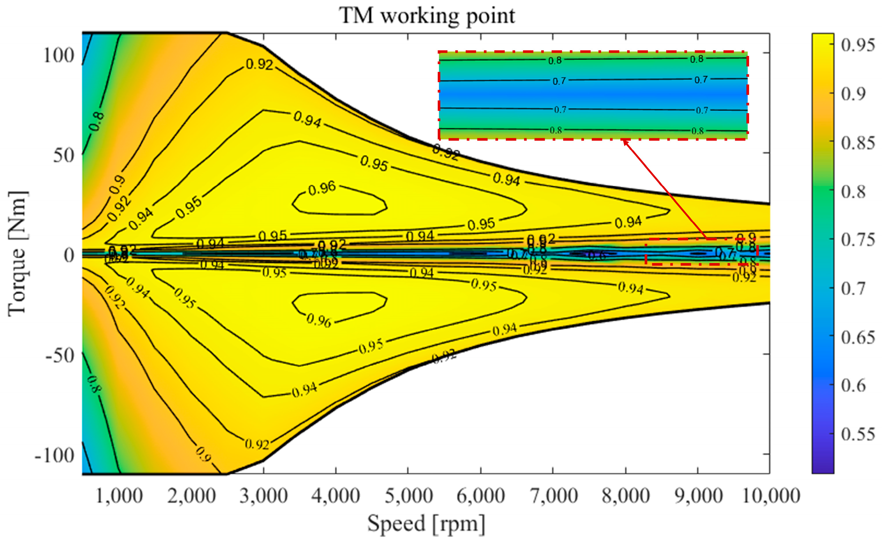
Utilizing the relevant data on the motor’s torque, speed, and efficiency, a motor MAP chart was constructed in MATLAB through interpolation. This chart employs speed as the horizontal axis and torque as the vertical axis, effectively illustrating the motor’s efficiency distribution across various speed and torque conditions. In the case of the dual-motor MAP chart, the datasets for Motors 1 and 2, which share identical parameters, have been halved. Figure 8 demonstrates that the overlay of Motors 1 and 2 retains the same external characteristics as those depicted in the original motor MAP chart.
2.2.2. Three Different Torque Allocation Schemes for the Dual-Motor EV
- (1)
- Scheme 1: Equal Torque Distribution between Dual Motors
During vehicle operation, the wheel torque is obtained from the wheel speed, and then, based on the powertrain route, the required torque for the motors is calculated. Motor 1 and Motor 2 each handle half of the required torque, meaning that each motor contributes half of the driving force.
The total duration of the operation is 18,000 s; represents the torque of Motor 1 and Motor 2 at each time step; and represents the total required torque at each time step.
- (2)
- Scheme 2: Single-Motor Priority
When the required torque falls within the operating range of Motor 1, it provides the entire torque and is responsible for driving. If the required torque exceeds the external characteristics of Motor 1, it provides its maximum torque, and the remaining torque is supplied by Motor 2.
where represents the maximum torque of Motor 1 at each time step.
- (3)
- Scheme 3: Dual-Motor Efficiency Optimization
At each time step, the required torque is distributed between Motor 1 and Motor 2 to minimize the instantaneous driving power or maximize the regenerative power, achieving both motors’ minimum total driving power throughout the entire operation.
At each moment, we first determine the lesser of the required torque and the allowable maximum torque . Based on this value, we generate a linearly distributed torque array consisting of 100 evenly spaced torque points. From this distribution, we select a specific torque that minimizes the driving power of Motor 1 at that instant, or maximizes the regenerative energy during braking. This torque is then allocated to Motor 1, with the remainder assigned to Motor 2.
where represents the torque of Motor 1 at each time step, taken from one of the 100 equally spaced values within the range of when the total required torque is more significant than zero, and within the range of when the total required torque is less than zero.
When the torque values of Motor 1 and Motor 2 are equally spaced and result in the minimum instantaneous total power, the torque is at that specific time step for Motor 1 and 2.
3. Simulation Results and Analysis of EV with Automated Manual Transmission
3.1. AMT EV Simulation Results and Analysis
The simulation results of the EV with AMT before and after optimization are organized in the order of single-stage main reducer, two-speed gearbox, three-speed gearbox, and four-speed gearbox. The data is presented for four aspects: electric energy consumption per 100 km; maximum vehicle speed; 0–100 km/h acceleration time; and maximum climbing slope, as shown in Table 7.
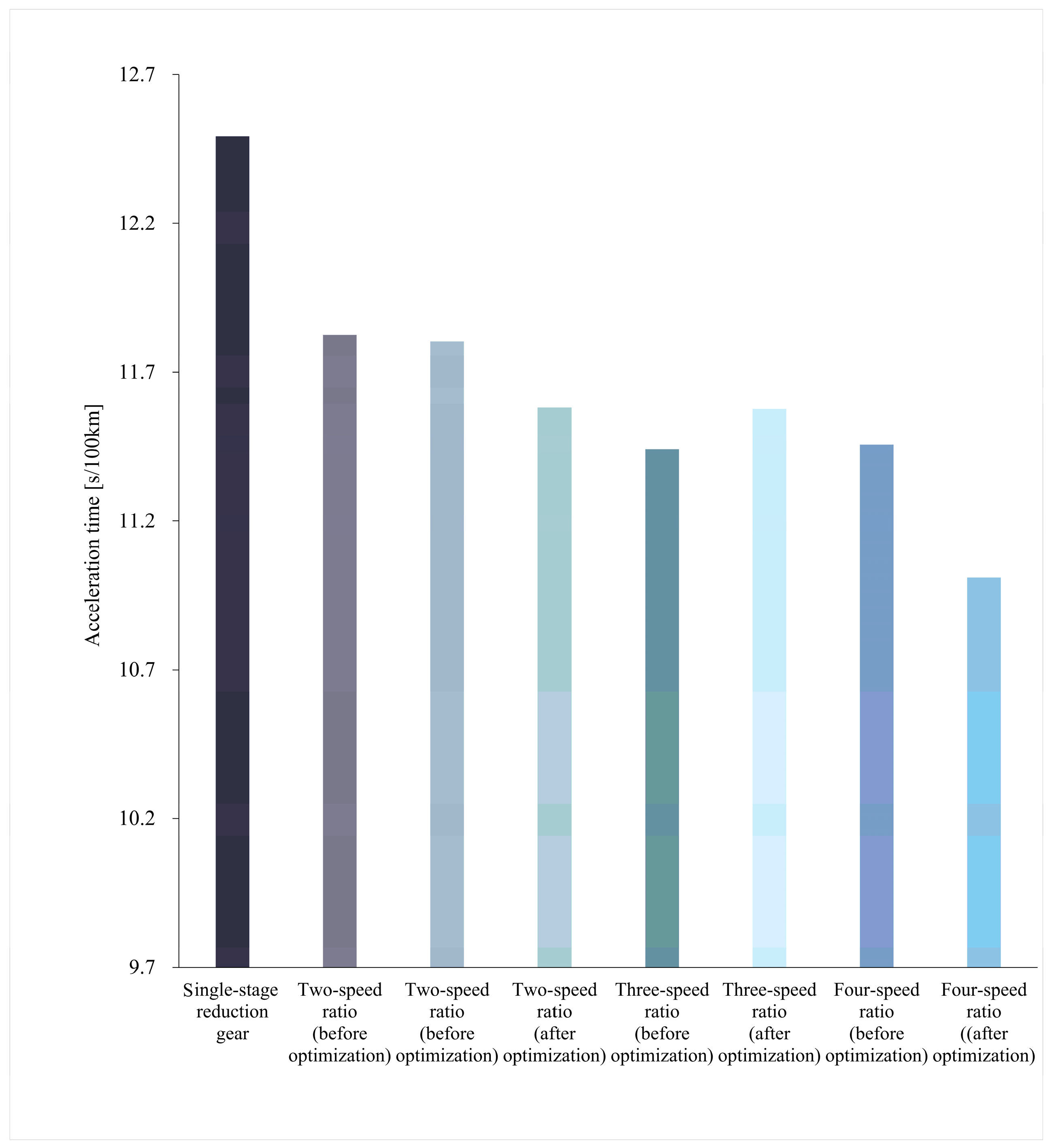
Data from Table 7 suggest that as the number of gearbox ratios increases, both the power performance and the economy of electric vehicles tend to decline. However, gear ratio optimization via genetic algorithms leads to some improvements in vehicle performance metrics, such as power consumption per hundred kilometers, maximum speed, acceleration time to one hundred kilometers, and maximum climbing gradient is shown in Figure 9, Figure 10, Figure 11 and Figure 12. Yet, the overall enhancement effect is somewhat limited. In the realm of power performance, electric vehicles featuring a four-speed gearbox markedly surpass those with a single-stage main reducer, although improvements in economy are not observed.
Upon analyzing the hundred-kilometer energy consumption across different gear transmissions, the optimized four-gear setup emerges as the most energy-efficient, with the three-gear setup trailing slightly behind. This suggests that, by adjusting the gear ratio, the transmission’s economic efficiency significantly benefits from an increased number of gears. Power performance metrics also favor the four-gear transmission, which, despite a minor reduction in maximum climbing capability post-optimization, still delivers the best overall power performance. These results underscore the critical role of gear ratio optimization in boosting both the economy and power performance of electric vehicles.
The energy consumption of single-stage main reducer EVs and the impact of optimization on EVs equipped with AMTs are presented above. The bar chart derived from simulation results reveals that optimizing the speed ratio leads to a decrease in energy consumption. However, the introduction of additional gears does not result in lower energy consumption for the EV.
To understand the reduction in energy consumption more deeply, we analyzed the energy losses and average efficiencies of the battery, motors, gearbox, and primary reducer. The detailed findings are provided in Table 8.
Simulation results indicate that while adding more gears to a vehicle enhances its dynamic performance, it reduces energy efficiency. However, fine-tuning the speed ratio and gear shifting speeds can boost both the vehicle’s economy and dynamics. Despite these optimizations, the economic performance of an EV equipped with AMT remains inferior to that of an EV with a single-level primary reducer.
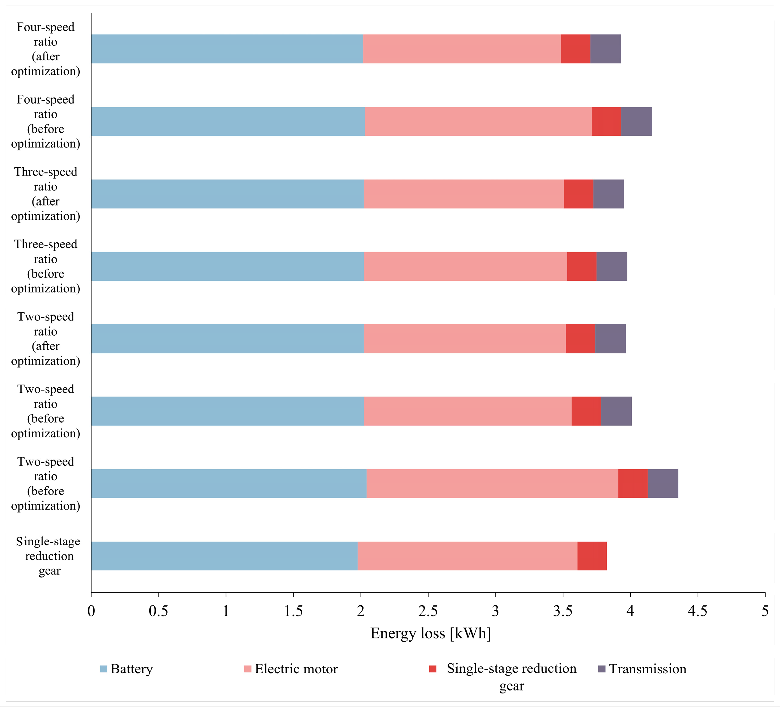
Further analysis on motor efficiency and energy losses shows that increasing the number of gears and optimizing speed ratios leads to higher average motor efficiency and reduced energy losses, specific details can be found in Figure 13 and Figure 14. Nonetheless, the motor efficiency of an EV with AMT still falls short when compared to an EV with a single-level primary reducer. This discrepancy stems from AMT’s extended energy transfer path, which causes a more significant increase in mechanical energy losses than the reduction in motor energy losses, leading to less favorable results. Additionally, AMT does not enhance the vehicle’s economy given the current motor performance, but instead degrades it.
This study also does not account for the potential increase in vehicle weight due to the inclusion of AMT, which could further diminish the vehicle’s economy. Therefore, the real potential for performance improvement with AMT might be less significant than the current findings suggest.
3.2. Double-Motor EV Simulation Results and Analysis
Based on the three different torque distribution schemes mentioned above, the model was constructed, and simulations were conducted by varying the scaling factors of Motor 1 and Motor 2.
The specific simulation results are shown in Table 9.
By calculating the energy losses and average efficiencies of the battery, Motor 1, Motor 2, and the primary reducer, the essence of the energy consumption reduction was analyzed, and the specific results are shown in Table 10.
Table 9 illustrates that increasing the proportion of Motor 1’s share leads to higher energy consumption in the dual-motor setup with equal torque distribution. The most efficient energy consumption, at 100 km, occurs when Motors 1 and 2 each hold a 0.5 share. Under both the single-motor priority and dual-motor efficiency-optimized schemes, energy consumption declines, reaching its lowest when Motor 1’s share is 0.7 and Motor 2’s is 0.3. These data allow for the determination of the optimal allocation of shares to Motor 1 and Motor 2, to achieve greater economic efficiency across three torque distribution schemes. Figure 15 demonstrates that the dual-motor efficiency-optimized scheme outperforms others in economic performance.
The strategy that emphasizes efficiency via dual-motor torque distribution shows that the battery and the motors maintain average efficiencies of 92.638%, 94.527%, and 94.694%, respectively. These figures represent improvements over the efficiencies of a system using a single-stage primary reducer exclusively, where the battery and motor efficiencies are 92.636% and 93.672%, respectively. As depicted in Figure 16 and Figure 17, operating Motor 1 and Motor 2 at a 0.5 ratio within the dual-motor efficiency-optimized scheme yields the highest average motor efficiency and minimal energy losses. Thus, this scheme significantly boosts the economic efficiency of electric vehicles.
4. Conclusions
This study conducted an in-depth efficiency analysis of EVs equipped with AMT and dual-motor configurations. Through simulation and optimization, it was found that although increasing the number of gears in AMT systems can enhance certain dynamic performances of the vehicle, it still falls short in energy efficiency compared to configurations with a single-stage main reducer. Consequently, under the current technological and market conditions, the adoption of one- or two-speed AMT configurations is more favored by the market. This choice boosts the dynamic performance of electric vehicles without significantly compromising economic efficiency.
On the other hand, the analysis of dual-motor configurations demonstrated that a rational torque distribution strategy could significantly improve the energy efficiency and driving experience of EVs. Implementing a dual-motor efficiency optimization scheme not only furthers the economic efficiency of electric vehicles, but also ensures robust dynamic performance. This discovery provides a new direction for the design of EV power systems.
This research highlights the need for meticulous optimization of AMT and dual-motor systems when designing efficient electric vehicles. While some initial results have been achieved, the evolution of EV technology is a continuous process of advancement. Future research may consider the following directions:
- Interdisciplinary Research: engaging in interdisciplinary collaboration across automotive engineering, motor control, and energy management teams to explore more efficient and intelligent EV power system designs.
- Intelligent Management Systems: developing EV energy management systems that integrate advanced control algorithms, enabling dynamic energy distribution based on real-time road conditions, driving habits, and energy consumption patterns.
- Environmental and Economic Win–Win: delving into the potential of electric vehicles to reduce environmental pollution and enhance energy use efficiency, contributing to the realization of sustainable transportation solutions.
Author Contributions
Z.W.: writing—original draft preparation. X.Q.: visualization. Q.C.: software. F.C.: investigation. J.W.: validation. D.S.: writing—reviewing and editing. All authors have read and agreed to the published version of the manuscript.
Funding
This research was funded by the Central Government to Guide Local Science and Technology Development Fund Projects of Hubei Province (2022BGE267), Hubei Superior and Distinctive Discipline Group of “New Energy Vehicle and Smart Transportation” (XKTD072023), the Independent Innovation Projects of the Hubei Longzhong Laboratory (2022ZZ-24).
Data Availability Statement
The original contributions presented in the study are included in the article, further inquiries can be directed to the corresponding author.
Conflicts of Interest
The authors declare no conflicts of interest.
References
- Jiang, J.; Zhu, S.; Wang, W.; Li, Y.; Li, N. Coupling coordination between new urbanisation and carbon emissions in China. Sci. Total Environ. 2022, 850, 158076. [Google Scholar] [CrossRef]
- Han, Y.; Duan, H.; Du, X.; Jiang, L. Chinese househ6old environmental footprint and its response to environmental awareness. Sci. Total Environ. 2021, 782, 146725. [Google Scholar] [CrossRef]
- Tamor, M.A.; Stechel, E.B. Electrification of transportation means a lot more than a lot more electric vehicles. iScience 2022, 25, 104376. [Google Scholar] [CrossRef]
- Hao, X.; Saafi, M.A.; Ou, S.; He, X.; Jiang, Y.; Lin, Z.; Yu, R.; Gan, Y.; Lu, Z. Assessing the cost-effectiveness of carbon neutrality for light-duty vehicle sector in China. iScience 2023, 26, 108203. [Google Scholar] [CrossRef] [PubMed]
- Alcázar-García, D.; Martínez, J.L.R. Model-based design validation and optimization of drive systems in electric, hybrid, plug-in hybrid and fuel cell vehicles. Energy 2022, 254, 123719. [Google Scholar] [CrossRef]
- Caban, J.; Małek, A.; Šarkan, B. Strategic Model for Charging a Fleet of Electric Vehicles with Energy from Renewable Energy Sources. Energies 2024, 17, 1264. [Google Scholar] [CrossRef]
- Piotrowska, K.; Piasecka, I.; Kłos, Z.; Marczuk, A.; Kasner, R. Assessment of the life cycle of a wind and photovoltaic power plant in the context of sustainable development of energy systems. Materials 2022, 15, 7778. [Google Scholar] [CrossRef]
- Dahbi, M.; Doubabi, S.; Rachid, A.; Oulad-Abbou, D. Performance evaluation of electric vehicle brushless direct current motor with a novel high-performance control strategy with experimental implementation. Proc. Inst. Mech. Eng. Part I J. Syst. Control Eng. 2020, 234, 358–369. [Google Scholar] [CrossRef]
- Fang, Y.; Ruan, J.; Walker, P.; Zhang, N. Comparison of effect on motor among 2-, 3-and 4-speed transmission in electric vehicle. In Proceedings of the 2017 IEEE International Conference on Mechatronics (ICM), Churchill, VIC, Australia, 13–15 February 2017. [Google Scholar]
- Kumar, V.; Chenchireddy, K.; Sreejyothi, K.R.; Sujatha, G. Design and Development of Brushless DC Motor Drive for Electrical Vehicle Application. In AI Enabled IoT for Electrification and Connected Transportation; Springer: Berlin/Heidelberg, Germany, 2022; pp. 201–217. [Google Scholar]
- Ganesan, A.; Murgovski, N.; Yang, D.; Gros, S. Real-Time Mixed-Integer Energy Management Strategy for Multi-Motor Electric Vehicles. In Proceedings of the 2023 IEEE Transportation Electrification Conference & Expo (ITEC), Detroit, MI, USA, 21–23 June 2023. [Google Scholar]
- Montazeri-Gh, M.; Pourbafarani, Z.; Mahmoodi-k, M. Comparative study of different types of PHEV optimal control strategies in real-world conditions. Proc. Inst. Mech. Eng. Part D J. Automob. Eng. 2018, 232, 1597–1610. [Google Scholar] [CrossRef]
- Ruan, J.; Walker, P.; Zhang, N. Comparison of power consumption efficiency of CVT and multi-speed transmissions for electric vehicle. Int. J. Automot. Eng. 2018, 9, 268–275. [Google Scholar] [CrossRef]
- Lin, X.; Li, Y.; Xia, B. An online driver behavior adaptive shift strategy for two-speed AMT electric vehicle based on dynamic corrected factor. Sustain. Energy Technol. Assess. 2021, 48, 101598. [Google Scholar] [CrossRef]
- He, B.; Chen, Y.; Wei, Q.; Wang, C.; Wei, C.; Li, X. Performance Comparison of Pure Electric Vehicles with Two-Speed Transmission and Adaptive Gear Shifting Strategy Design. Energies 2023, 16, 3007. [Google Scholar] [CrossRef]
- Shen, P.; Zhao, Z.; Guo, Q.; Zhou, P. Development Of economic velocity planning algorithm for plug-in hybrid electric vehicle. IEEE Trans. Intell. Transp. Syst. 2021, 23, 5501–5513. [Google Scholar] [CrossRef]
- Borthakur, S.; Subramanian, S.C. Design and optimization of a modified series hybrid electric vehicle powertrain. Proc. Inst. Mech. Eng. Part D J. Automob. Eng. 2019, 233, 1419–1435. [Google Scholar] [CrossRef]
- Ganesan, A.; Gros, S.; Murgovski, N. Numerical Strategies for Mixed-Integer Optimization of Power-Split and Gear Selection in Hybrid Electric Vehicles. IEEE Trans. Intell. Transp. Syst. 2022, 24, 3194–3210. [Google Scholar] [CrossRef]
- Fu, J.; Song, S.; Fu, Z.; Ma, J. Design of coordinated control strategy during driving mode switching for parallel hybrid electric vehicles. Trans. Inst. Meas. Control 2019, 41, 2507–2520. [Google Scholar] [CrossRef]
- Li, Y.; Zhu, B.; Zhang, N.; Peng, H.; Chen, Y. Parameters optimization of two-speed powertrain of electric vehicle based on genetic algorithm. Adv. Mech. Eng. 2020, 12, 1687814020901652. [Google Scholar] [CrossRef]
- Korayem, A.H.; Khajepour, A.; Fidan, B. A review on vehicle-trailer state and parameter estimation. IEEE Trans. Intell. Transp. Syst. 2021, 23, 5993–6010. [Google Scholar] [CrossRef]
- Panyam, A.R.; Panguluru, C. Design Parameter Optimization of Electric Drive Units. A Regression Based Optimization of PMSM Geometrical Design Parameters and Final Drive Ratio. Master’s Thesis, Chalmers University of Technology, Gothenburg, Sweden, 2023. [Google Scholar]
- Yu, X.; Lin, C.; Zhao, M.; Yi, J.; Su, Y.; Liu, H. Optimal energy management strategy of a novel hybrid dual-motor transmission system for electric vehicles. Appl. Energy 2022, 321, 119395. [Google Scholar] [CrossRef]
- Tian, Y.; Yi, G.; Ji, X.; Wen, G.; Zhang, Y.; Liu, J.; Zhang, N. Design, Analysis and Mode Shifting of a Novel Dual-Motor Powertrain for electric vehicles. IEEE Trans. Transp. Electrif. 2023. [Google Scholar] [CrossRef]
- Wang, Z.; Zhou, J.; Rizzoni, G. A review of architectures and control strategies of dual-motor coupling powertrain systems for battery electric vehicles. Renew. Sustain. Energy Rev. 2022, 162, 112455. [Google Scholar] [CrossRef]
- Zhu, L.; Tao, F.; Fu, Z.; Wang, N.; Ji, B.; Dong, Y. Optimization based adaptive cruise control and energy management strategy for connected and automated FCHEV. IEEE Trans. Intell. Transp. Syst. 2022, 23, 21620–21629. [Google Scholar] [CrossRef]
- Hu, J.; Zheng, L.; Jia, M.; Zhang, Y.; Pang, T. Optimization and model validation of operation control strategies for a novel dual-motor coupling-propulsion pure electric vehicle. Energies 2018, 11, 754. [Google Scholar] [CrossRef]
- Nguyen, C.T.; Walker, P.D.; Zhang, N. Optimization and coordinated control of gear shift and mode transition for a dual-motor electric vehicle. Mech. Syst. Signal Process. 2021, 158, 107731. [Google Scholar] [CrossRef]
- Wang, Y.; Cai, H.; Liao, Y.; Gao, J. Study on global parameters optimization of dual-drive powertrain system of pure electric vehicle based on multiple condition computer simulation. Complexity 2020, 2020, 6057870. [Google Scholar] [CrossRef]
- Hu, J.; Zu, G.; Jia, M.; Niu, X. Parameter matching and optimal energy management for a novel dual-motor multi-modes powertrain system. Mech. Syst. Signal Process. 2019, 116, 113–128. [Google Scholar] [CrossRef]
- Tian, Y.; Zhang, N.; Zhou, S.; Walker, P.D. Model and gear shifting control of a novel two-speed transmission for battery electric vehicles. Mech. Mach. Theory 2020, 152, 103902. [Google Scholar] [CrossRef]
- Zhao, H.; Liu, K.; Li, S.; Yang, F.; Cheng, S.; Eldeeb, H.H.; Kang, J.; Xu, G. Shielding optimization of IPT system based on genetic algorithm for efficiency promotion in EV wireless charging applications. IEEE Trans. Ind. Appl. 2021, 58, 1190–1200. [Google Scholar] [CrossRef]
- Ahssan, M.R.; Ektesabi, M.; Gorji, S. Gear ratio optimization along with a novel gearshift scheduling strategy for a two-speed transmission system in electric vehicle. Energies 2020, 13, 5073. [Google Scholar] [CrossRef]
Figure 1.
Single-stage main reducer EV powertrain architecture diagram.

Figure 2.
Motor external characteristic diagram.

Figure 3.
First-order equivalent circuit diagram.

Figure 4.
Battery discharge characteristic diagram.

Figure 5.
EV with Automated Manual Transmission powertrain architecture diagram.

Figure 6.
Genetic algorithm flowchart.

Figure 7.
Dual-motor EV powertrain architecture diagram.

Figure 8.
Motor MAP reduced by 50%.

Figure 9.
Comparison of 100 km electric consumption between single-stage main reducer and AMT.

Figure 10.
Comparison of maximum vehicle speeds between single-stage main reducer and AMT.

Figure 11.
Comparison of 0–100 km acceleration times between single-stage main reducer and AMT.

Figure 12.
Comparison of maximum gradients between single-stage main reducer and AMT.

Figure 13.
Comparison of average efficiencies of key components between single-stage main reducer and AMT.
Figure 13.
Comparison of average efficiencies of key components between single-stage main reducer and AMT.

Figure 14.
Comparison of energy losses of key components between single-stage main reducer and AMT.

Figure 15.
Comparison of 100 km electric consumption among different double-motor schemes.

Figure 16.
Comparison of average efficiencies of key components among different double-motor schemes.
Figure 16.
Comparison of average efficiencies of key components among different double-motor schemes.

Figure 17.
Comparison of energy losses of key components among different double-motor schemes.


Table 1.
Basic parameters of the vehicle.
| Technical Parameters | Reference Value |
|---|---|
| Length × Width × Height (mm) | 4070 × 1770 × 1570 |
| Curb Weight (kg) | 1285 |
| Minimum Ground Clearance (mm) | 150 |
| Rolling Resistance Coefficient | 0.0085/0.0018/0.00028 |
| Frontal Area (m2) | 2.513 |
| Tire Rolling Radius (m) | 0.31 |
| Rotating Mass Conversion Coefficient | 1.03 |
| Aerodynamic Drag Coefficient | 0.28 |
| Air Density (kg/m3) | 1.19 |
Table 2.
Design objectives.
| Performance | Design Objective | Value |
|---|---|---|
| Dynamic performance | Maximum Vehicle Speed (km/h) | >140 |
| 0~100 km/h Acceleration Time (s) | <13 | |
| Maximum Gradeability (%) | >30 | |
| Electric consumption | Electric energy consumption per 100 km under China light-duty vehicle test cycle (CLTC) conditions (kWh/100 km) | <9.96600 |
Table 3.
Simulation results.
| Performance | Design Objective | Value |
|---|---|---|
| Dynamic performance | Maximum Vehicle Speed (km/h) | 159.20000 |
| 0~100 km/h Acceleration Time (s) | 12.49260 | |
| Maximum Gradeability (%) | 37.43000 | |
| Electric consumption | Electric energy consumption per 100 km under CLTC conditions (kWh/100 km) | 9.79640 |
Table 4.
Gear ratios and shift speeds of AMT in various gears.
| Type | Gear Ratio | Shift Speed (km/h) |
|---|---|---|
| 2-Speed AMT | 1.5/1 | 60 |
| 2-Speed AMT | 1/0.75 | 60 |
| 3-Speed AMT | 1.25/1/0.75 | 40/80 |
| 4-Speed AMT | 1.5/1.25/1/0.75 | 30/60/90 |
Table 5.
Specific parameter settings for the genetic algorithm.
| Type | Gear Ratio | Shift Speed (km/h) | |||||
|---|---|---|---|---|---|---|---|
| 2-Speed AMT | 1–1.25 | 0.75–1 | 40–60 | ||||
| 3-Speed AMT | 1.375–1.125 | 1.125–0.875 | 0.875–0.625 | 30–45 | 45–90 | ||
| 4-Speed AMT | 1.375–1.125 | 1.125–1 | 1–0.875 | 0.875–0.625 | 30–45 | 45–70 | 70–90 |
Table 6.
Specific data for each gear of AMT after optimization.
| Type | Gear Ratio | Shift Speed (km/h) | Optimal Electric Consumption (kWh/100 km) | |||||
|---|---|---|---|---|---|---|---|---|
| 2-Speed AMT | 1.14480 | 0.75000 | 41.97700 | 9.89130 | ||||
| 3-Speed AMT | 1.35500 | 0.91000 | 0.73800 | 32.16900 | 55.37300 | 9.88190 | ||
| 4-Speed AMT | 1.35540 | 1.00860 | 0.87500 | 0.62510 | 30.24160 | 45.00410 | 75.00730 | 9.8671 |
Table 7.
Simulation results of EV with AMT.
| Electric Energy Consumption per 100 km (kWh/100 km) | Maximum Vehicle Speed (km/h) | 0~100 km/h Acceleration Time (s) | Maximum Gradeability (%) | |
|---|---|---|---|---|
| Single-Motor Primary Reducer | 9.79640 | 159.20000 | 12.49260 | 37.43000 |
| Before Optimization—Two Gears | 10.15250 | 158.30000 | 11.82540 | 62.74000 |
| Before Optimization—Two Gears | 9.92060 | 162.40000 | 11.80340 | 37.43000 |
| After Optimization—Two Gears | 9.89130 | 162.40000 | 11.58140 | 44.02000 |
| Before Optimization—Three Gears | 9.89770 | 162.40000 | 11.44220 | 49.13000 |
| After Optimization—Three Gears | 9.88190 | 162.60000 | 11.57680 | 54.56000 |
| Before Optimization—Four Gears | 10.02040 | 162.40000 | 11.45740 | 62.74000 |
| After Optimization—Four Gears | 9.86710 | 164.50000 | 11.01080 | 54.58000 |
Table 8.
Energy losses and average efficiencies of key components in EV with AMT.
| Battery | Electric Motor | Main Reducer | AMT | ||
|---|---|---|---|---|---|
| Single-Motor Primary Reducer | Energy loss | 1.97646 | 1.63030 | 0.21842 | |
| Average efficiency | 0.92636 | 0.93672 | 0.98039 | ||
| Before Optimization—Two Gears | Energy loss | 2.04247 | 1.86692 | 0.21842 | 0.22733 |
| Average efficiency | 0.92585 | 0.92943 | 0.98039 | 0.98000 | |
| Before Optimization—Two Gears | Energy loss | 2.02277 | 1.54141 | 0.21842 | 0.22733 |
| Average efficiency | 0.92596 | 0.94115 | 0.98039 | 0.98000 | |
| After Optimization—Two Gears | Energy loss | 2.02149 | 1.49911 | 0.21842 | 0.22733 |
| Average efficiency | 0.92595 | 0.94269 | 0.98039 | 0.98000 | |
| Before Optimization—Three Gears | Energy loss | 2.02204 | 1.50812 | 0.21842 | 0.22733 |
| Average efficiency | 0.92596 | 0.94237 | 0.98039 | 0.98000 | |
| After Optimization—Three Gears | Energy loss | 2.02120 | 1.48535 | 0.21842 | 0.22733 |
| Average efficiency | 0.92595 | 0.94320 | 0.98039 | 0.98000 | |
| Before Optimization—Four Gears | Energy loss | 2.03019 | 1.68250 | 0.21842 | 0.22733 |
| Average efficiency | 0.92596 | 0.93605 | 0.98039 | 0.98000 | |
| After Optimization—Four Gears | Energy loss | 2.01877 | 1.46577 | 0.21842 | 0.22733 |
| Average efficiency | 0.92599 | 0.94391 | 0.98039 | 0.98000 |
Table 9.
Simulation results of double-motor EV.
| Motor Scaling Ratio | Electric Energy Consumption per 100 km (kWh/100 km) | ||
|---|---|---|---|
| Equal Torque Distribution between Dual Motors | Single Motor Priority | Dual-Motor Efficiency Optimization | |
| (TM1 0.5, TM2 0.5) | 9.79640 | 9.85810 | 9.61830 |
| (TM1 0.55, TM2 0.45) | 9.80800 | 9.82640 | 9.60270 |
| (TM1 0.6, TM2 0.4) | 9.82610 | 9.77700 | 9.58130 |
| (TM1 0.7, TM2 0.3) | 9.89360 | 9.75820 | 9.57510 |
Table 10.
Energy losses and average efficiencies of key components in double-motor EV.
| Battery | Electric Motor 1 | Electric Motor 2 | Main Reducer | ||
|---|---|---|---|---|---|
| Equal Torque Distribution between DualMotors | Energy loss | 1.97646 | 0.81515 | 0.81515 | 0.21842 |
| Average efficiency | 0.92636 | 0.93672 | 0.93672 | 0.98039 | |
| Single-Motor Priority | Energy loss | 1.99093 | 1.66425 | 0.04331 | 0.21842 |
| Average efficiency | 0.92596 | 0.93410 | 0.92307 | 0.98039 | |
| Dual-Motor Efficiency Optimization | Energy loss | 1.96765 | 0.53875 | 0.83519 | 0.21842 |
| Average efficiency | 0.92638 | 0.94527 | 0.94694 | 0.98039 |
Disclaimer/Publisher’s Note: The statements, opinions and data contained in all publications are solely those of the individual author(s) and contributor(s) and not of MDPI and/or the editor(s). MDPI and/or the editor(s) disclaim responsibility for any injury to people or property resulting from any ideas, methods, instructions or products referred to in the content. |
© 2024 by the authors. Licensee MDPI, Basel, Switzerland. This article is an open access article distributed under the terms and conditions of the Creative Commons Attribution (CC BY) license (https://creativecommons.org/licenses/by/4.0/).
Share and Cite
MDPI and ACS Style
Wang, Z.; Qu, X.; Cai, Q.; Chu, F.; Wang, J.; Shi, D. Efficiency Analysis of Electric Vehicles with AMT and Dual-Motor Systems. World Electr. Veh. J. 2024, 15, 182. https://doi.org/10.3390/wevj15050182
AMA Style
Wang Z, Qu X, Cai Q, Chu F, Wang J, Shi D. Efficiency Analysis of Electric Vehicles with AMT and Dual-Motor Systems. World Electric Vehicle Journal. 2024; 15(5):182. https://doi.org/10.3390/wevj15050182
Chicago/Turabian StyleWang, Zhenghong, Xudong Qu, Qingling Cai, Fulin Chu, Jiaheng Wang, and Dapai Shi. 2024. "Efficiency Analysis of Electric Vehicles with AMT and Dual-Motor Systems" World Electric Vehicle Journal 15, no. 5: 182. https://doi.org/10.3390/wevj15050182