Article

Elevational Earth-Sheltered Buildings with Horizontal Overhang Photovoltaic-Integrated Panels—New Energy-Plus Building Concept in the Territory of Serbia

1
Faculty of Engineering, University of Kragujevac, Sestre Janjić 6, 34000 Kragujevac, Serbia
2
Faculty of Environmental Engineering, Geodesy and Renewable Energy, Kielce University of Technology, al. Tysiaclecia P.P. 7, 25-314 Kielce, Poland
3
Faculty of Mechatronics and Mechanical Engineering, Kielce University of Technology, al. Tysiaclecia P.P. 7, 25-314 Kielce, Poland
*
Author to whom correspondence should be addressed.
Energies 2024, 17(9), 2100; https://doi.org/10.3390/en17092100
Submission received: 15 March 2024 / Revised: 18 April 2024 / Accepted: 22 April 2024 / Published: 27 April 2024
(This article belongs to the Special Issue Energy Efficiency of the Buildings III)

Abstract

:
The global scientific community is intensively promoting energy-plus buildings. Following the leading world trends, this paper presents a new energy-plus building concept—elevational earth-sheltered buildings with three different types of horizontal overhang photovoltaic-integrated panels: wooden support columns covered with clay tiles, steel pipes as support columns covered with sheet steel, and concrete support columns with concrete coverage. In this instance, the specific multi-numerical case study building model for the city of Kragujevac (located in central Serbia with favorable climatic conditions) was performed over 7 months (from 1 October to 30 April), taking into account the soil temperature, the effects of solar shading, the performance of the heating system—a ground source heat pump—and the characteristics of the artificial and automatic lighting control system. The simulation results show that the optimal depth of a horizontal overhang (energy-plus status) depends on the occupant’s habits, in addition to meteorological conditions. The presented methodology can be used for any other location, both in Europe and the world.

1. Introduction

The development of the concept of energy-efficient buildings (EEBs) arose from the need to bring the (primarily) residential sector closer to sustainable development [1]. However, certain studies for the year 2021 showed that the EU residential sector uses 24.7% of the total final energy consumption [2]. The greatest amount of this energy is used for heating (64.4% [3]). The Serbia residential sector, with a share of 35.8% [2], is in a more difficult situation, although several legal documents in the field of energy efficiency (for example, building energy ratings (BERs)) have been prescribed and adopted since the beginning of the 21st century [4]. As time goes on, it is certain that the EU energy community will be increasingly strict about final energy consumption in the residential sector and will work even more intensively to implement EEBs (Figure 1). The mentioned trends will not bypass Serbia either, so it is desirable to catch the connection as soon as possible because the existing buildings will be in an increasingly unfavorable position.
Today, great attention is paid to the shape of buildings [6,7], their orientation [8,9], the mutual distance between buildings and building density [10,11], vegetation use [12,13], maximization of daylight use [14,15], the use of modern construction materials [16,17], and shading devices, which will be chronologically (from 1998 to 2024) analyzed below. In [18], the effects of passive cooling using window overhangs for a building located in Shiraz (Iran) were investigated experimentally and theoretically. The results of a 1998 study showed that the annual final energy consumption for cooling can be reduced by over 12%. The paper also determined the optimal dimensions of overhangs for buildings located at latitudes of about 29.6° N. In 2005, Ossen et al. used a dynamic energy simulation program supported by the DOE2.2 calculation engine to determine the energy consumption for artificial lighting because the overhangs reduce the level of daylight [19]. In a review paper published in 2012, the effects of building shading and their importance for energy savings were analyzed [20].
Determining the optimal dimensions of overhangs above windows on the south facade wall of a building physically made in line with energy efficiency recommendations for the area of Souidania (Algeria) is presented in [21]. In addition to the experimental approach, numerical dynamic simulations (using TRNSYS 16 software EnergyPlus 7.1) were also used in this paper. In the same year (2014), the effects of window shading on high-rise buildings were published in two papers. The first high-rise building was located in Seoul (Republic of Korea) [22]. The second high-rise building was located in Taipei (Taiwan) [23]. For example, the results in [22] showed that the final energy consumption for cooling can be reduced by more than 20%. One more review paper (for different types of shading devices for windows [24]) was published in 2014. Two interesting papers [25,26] were published in 2016. In [25], the use of overhangs as a potential building facade for improving single-sided ventilation performance was analyzed. The influence of horizontal overhangs (HOs) and glazing with special spectral radiative properties on the annual thermal balance of buildings, as well as the thermal and visual comfort of the users, is presented in [26].
Research from 2017, available in [27], focused on the effects of passive cooling and the effects of passive heating. The authors concluded that the overhangs could, on the one hand, reduce the annual final energy consumption for cooling, but they could also increase the annual final energy consumption for heating on the other hand. In other words, the optimal dimensions of the overhangs should be carefully determined. Bojić et al. [28] used the Hooke-Jeeves algorithm and the EnergyPlus 7.0 software Google SketchUp 8 to numerically determine the optimal depth of HOs for a residential building located in Belgrade (Serbia). Concrete HOs were positioned on all facade walls. The simulations were performed during the summer period, so only cooling energy consumption was monitored. The optimization algorithm used takes into account embodied energy and primary energy. A review of energy savings using solar control techniques and optimal building orientation for the strategic placement of facade shading systems is presented in [29].
The possibility of using shading devices in the educational building in Madurai (India) was investigated in [30] in 2018.
Unlike most works, Liu et al. [31] paid attention to nontransparent facades and their shading to achieve energy savings (study from 2019). They used various types of horizontal and vertical shading devices, with different positional angles about the facade walls, to show that the greatest energy savings (up to 8%) are achieved by shading the western nontransparent facade walls. Rashid et al. investigated the redistribution of energy flows for three thermo-technical systems (passive cooling, artificial lighting, and mechanical cooling) for three types of external sun shading devices (one HO, multi-vertical fins, and an egg-crate device) [32].
The results of Sghiouri et al. (2020) showed that automated movable shading in the building located in Maroco is the most effective solution for passive cooling [33]. The research presented in [34] by Nikolić et al., in fact, is a continuation of the research presented in [28]. Here, the subject of numerical research (also using the Hooke-Jeeves algorithm and EnergyPlus software) was a building (also located in Belgrade, Serbia) with two floors. The shading devices were balconies (for the ground floor) and roofs (for the first floor). With optimal dimensions for the mentioned HOs, the annual total primary energy consumption (for heating, cooling, and lighting) can be reduced by over 7%.
In 2021, Krarty compared movable (with different working principles) and fixed window shading devices that would be applied to US buildings in Phoenix and San Francisco [35]. The advantage of movable shading devices over fixed ones depends on the size and type (number of layers, type of material, etc.) of the window, their orientation, and weather conditions (time of day and year). Mobile shading devices can save 45% more energy for air conditioning compared to fixed shading devices for buildings with a window–wall ratio of 30%. In [36], Krarti continued his research in the area of solar shading. He placed PV panels on movable superstructures with a horizontal axis. If such devices were placed above the windows on the southern facade walls, the energy savings would be up to 6% for overhangs without PV panels and up to 35% for overhangs with PV panels. In general, for locations with warm climates, the savings could be over 90%.
Koç et al. [37] created 1485 scenarios with fixed shading devices to reduce the final energy consumption for cooling an office building in Turkey (a study published in 2022). By using a comprehensive approach, they managed to reduce the annual final energy consumption for cooling by 70%. Mohammed et al. installed seven types of shading devices on the Darwin town hall building (Australia) and achieved savings of 15.5% [38].
In 2023, two interesting papers were published. Corti et al. [39] presented a review work of external integrated systems as photovoltaic (PV) shading devices, while [40] presented a design framework of an automatic shading device based on a sun path diagram.
Dong-Hyun et al. (a study from 2024) presented a paper [41] that proposes a high-precision methodology for optimizing dynamic shading device systems using the genetic optimization algorithm. Jiang et al. [42] analyzed energy consumption and daylighting control in office buildings using dynamic PV shading devices. Energy savings in office buildings can be achieved between 32.13–50.38%.
It is clear that in the future, EEBs will strive to maximize the passive use of renewable energy, primarily solar energy, geothermal energy, and wind energy. It can also be expected that the bioclimatic-passive strategy, which promotes the use of earth-sheltered buildings (ESBs) [43,44], again, becomes a subject of wider interest, although it has always been used in human civilization as a construction concept.
The scientific community is working hard to popularize ESBs. In the recent past, the energy, environmental, and economic performance of these buildings have been the subject of many studies and projects in different countries: Nigeria [44], China [45], Egypt [46], Russia [47], the USA [48], Brazil [49], Iran [50], etc. On the other side, the negligible presence of ESBs on the territory of Serbia (despite a certain number of works by Milanović [51,52] and Nešović [53,54]), both in traditional and contemporary architecture, has a multi-layered background: historical, cultural, sociological, economic, climatic, typological, and pedological. Although thermal comfort has been positively evaluated, high investment costs, problems with moisture, sound and visual effects, etc., have, in the past, created another negative background in terms of structural elements. The current rulebook on the classification of buildings in Serbia [4] does not recognize ESBs. The same applies to other accompanying legal documents.
In this paper, the subject of research is elevational earth-sheltered buildings (ESBs) with horizontal overhang photovoltaic-integrated (HOPVI) panels. The authors think that a bioclimatic-passive strategy combined with a passive solar shading device (HO), energy-efficient thermo-technical systems (PV panels, a ground source heat pump (GSHP), and an artificial and automatic lighting control system (AALCS)), as well as people’s responsible habits, can reach EPB status. In other words, drawing the attention of the scientific public to the great importance of ESBs using HOPVI panels as future EEB trends is the main motive of this research.
The work is based on numerical simulations. The EnergyPlus software uses the finite difference method (FDM) to determine energy flows in ESB with HOPVI panels, while the Siemens Femap 2020 software Siemens Femap 2020 uses the finite element method (FEM) to determine the degree of safety of shading devices (the first novelty in this research).
According to the comments given in [27], the potential EPB status of ESBs using HOPVI panels was investigated during the heating season (from 1 October to 30 April) in a moderate continental climate (the second novelty). Contrary to [28], a breakthrough was also made because three completely different types of HOs were considered (the third novelty): wooden support columns covered with clay tiles (first model), steel pipe support columns covered with sheet steel (second model), and concrete support columns with concrete cover (third model).
The energy and ecological indicators of ESBs using HOPVI panels were determined and are presented here: final energy consumption, primary energy consumption, CO2 emission, embodied energy, and total energy consumption.

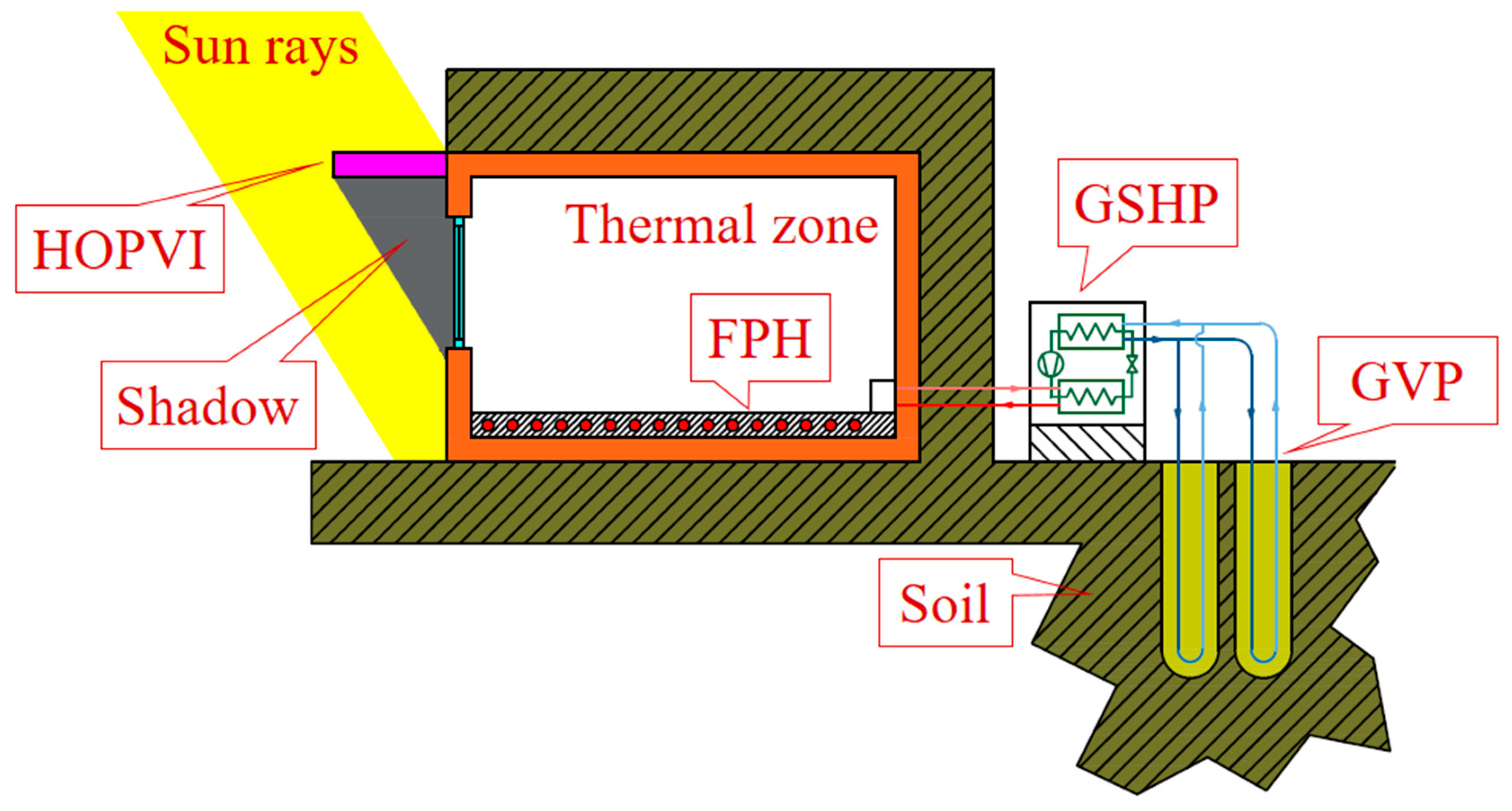
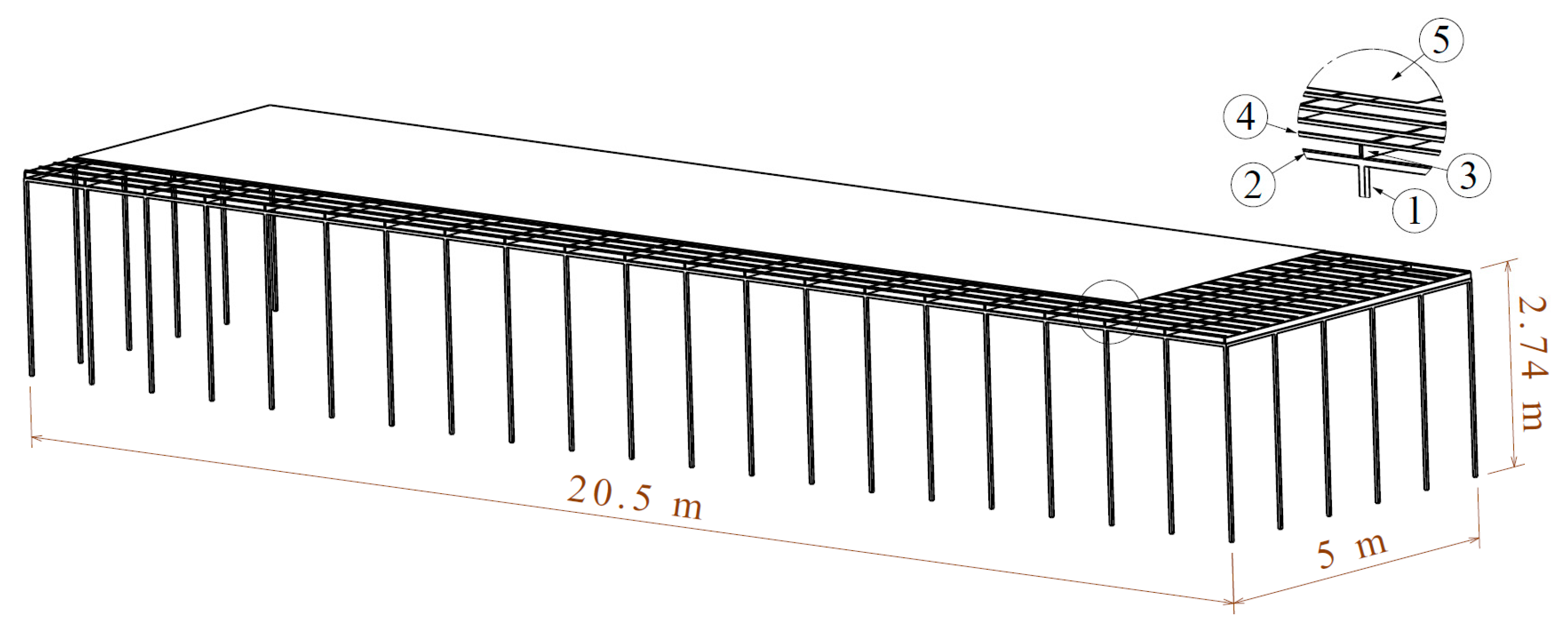
2. Description of the Elevational Earth-Sheltered Buildings

2.1. Construction Physics

The subject of the research is elevational ESBs (Figure 2). The length of the building is 20.5 m, the width is 5 m, and the height is 2.6 m. The total area is Aesb,gf,tot = 102.5 m2. The form factor is Aesb,tot/Vesb,tot = 1.267 l/m, while the window–wall ratio (WWR) is Aesb,ww,tot/Aebs,wl,tot = 0.16 for the south, free facade. An isometric view of an elevational ESB is shown in Figure 2.
A family of four lives in the elevational ESB all year round. The building consists of eight rooms, i.e., thermal zones (Figure 3): BDR1 (17.5 m2), BDR2 (9 m2), BDR3 (9 m2), BAT (6 m2), H (26 m2), LR (25 m2), K (6 m2), and SR (4 m2). BDR1 is intended for the parents, while each child has their room (BDR2 and BDR3). According to basic architectural principles, all rooms (except SR) are exposed to the Sun by the southern facade wall, so all transparent elements (windows and entrance door) are positioned on them.
The elevational ESB is modeled on the Rulebook on Energy Efficiency of New Buildings [4]. The adopted values for the air change for each thermal zone nz [h−1] are the following: nz = 0.5 l/h (BDR1, BDR2, BDR3, H, LR, and SR) and nz = 1.5 l/h (BAT and K). The adopted Uad [W/(m2K)] and allowed, i.e., maximum Umax [W/(m2K)], values for all the construction elements of the analyzed building are presented in Table 1.

2.2. Performance of the Heating System

During the analyzed period (from 1 October to 30 April), 98.5 m2 of the elevational ESB was thermally treated (SR is an unheated room, Figure 3).
The central heating system using a GSHP was selected (Figure 4). The coefficient of performance COP [-] of the GSHP is COP = 4.56. The nominal power of the condenser is 7.3 kW. The nominal power of the compressor is 1.6 kW. On the outside, the GSHP is connected to two geothermal vertical probes (GVPs). The depth of the GVPs is 73.2 m (each), so the total nominal power is 5.7 kW.
Each room (on the inside) is equipped with a suitable floor panel heater (FPH) and a thermostat (Figure 4). The thermostat regulates the mass flow rate of the working fluid (water) to maintain the desired internal ambient temperature (20 °C, valid for all heated rooms).

2.3. Performance of the Lighting System

Each room (except SR) is equipped with artificial lighting (AL). In this case, surface-mount lights (SMLs) were adopted. The technical characteristics of SMLs (according to the recommendations from [55]) are presented in Table 2.
All rooms with SMLs are equipped with day-lighting control systems (DLCSs). The DLCS measures the intensity of solar illuminance through a reference point. In Figure 5 (example for LR), it can be seen that the DLCS device (reference point) is located in the middle of the room and at a height of 800 mm (this applies to each room, except for H and SR).
The DLCS and SML are interconnected within each zone. When the solar illuminance is not sufficient to achieve optimal values, i.e., set values (Table 2), then the DLCD activates the SML, which supplements this difference artificially (with electricity consumption). The SML and DLCS together form the artificial and automatic lighting control system (AALCS). The working time of the AALCS during the analyzed period was from 06:00 to 22:00.

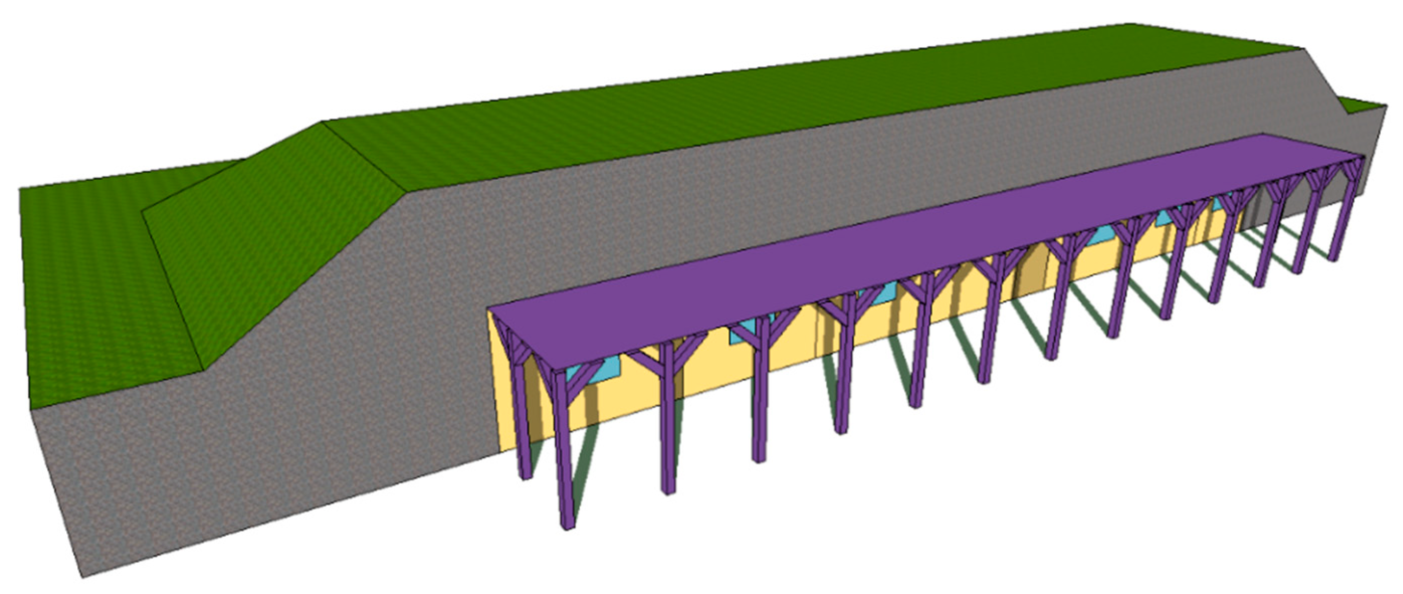
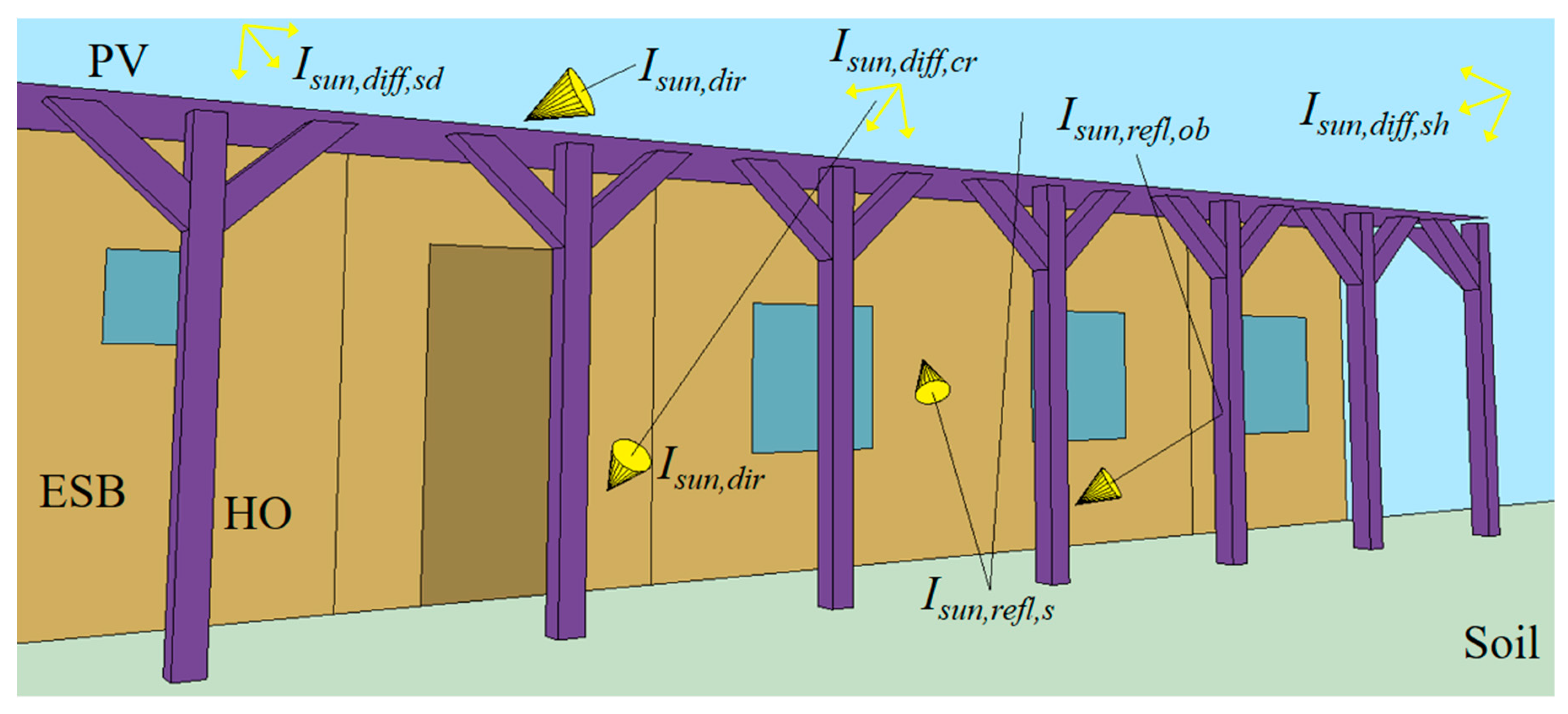
3. Description of the Horizontal Overhang Integrated Photovoltaic Panels

3.1. Performance of the Horizontal Overhangs

The following types of HOs are most often used in the city of Kragujevac: wooden support columns covered with clay tiles, steel pipe support columns covered with sheet steel, and concrete support columns with concrete coverage. Accordingly, in the following figures (Figure 6, Figure 7 and Figure 8), corresponding models of HOs were created: model HO-1 (Figure 6), model HO-2 (Figure 7), and model HO-3 (Figure 8), respectively.
In order to create the HO-1 model at a total height of 2.9, the following profiles were used (Figure 6): vertical wooden posts with hairpins (1) and horizontal wooden beams (2) with a square cross-section of 150 × 150 mm, horizontal slats with cross-sections of 100 × 50 mm (3) and 50 × 50 mm (4). The overhang is covered with clay titles (5) with a thickness of 25 mm.
The geometric characteristics of the HO-2 model are the following (Figure 7): vertical (1) and horizontal (2) steel pipes with a square cross-section of 40 × 40 × 1.5 mm, steel pipes (3) with a rectangular cross-section of 80 × 20 × 2.5 mm, steel pipes (4) with a square cross-section of 20 × 20 × 1.5 mm, and steel sheets (5) with a thickness of 0.5 mm.
The HO-3 model has the simplest design (Figure 8). The vertical concrete columns (1) have a square cross-section of 200 × 200 mm, and the horizontal concrete slab (2) is 100 mm thick.
The mechanical and thermal characteristics of the supporting columns and covers for the different models of HOs (HO-1, HO-2, and HO-3) are presented in Table 3.
According to the recommendations from [61], the production of steel sheets requires the greatest energy investment (97.6 MJ/kg; Table 3). In second place is the production of steel pipes (38.8 MJ/kg). In third place are the wooden elements (26.9 MJ/kg). On the other hand, HO-3 consumes the least amount of energy (1.1 MJ/kg, Table 3).

3.2. Performance of the Photovoltaic Panels

Solar radiation is incoming onto horizontally placed PV panels—according to the design of the HOs (Figure 6, Figure 7 and Figure 8). The PV panels cover the upper surface of the HOs (HOPVI design). The efficiency of the PV panels is 20% (adopted value), and the embodied energy is 585 kWh/m2 [62].

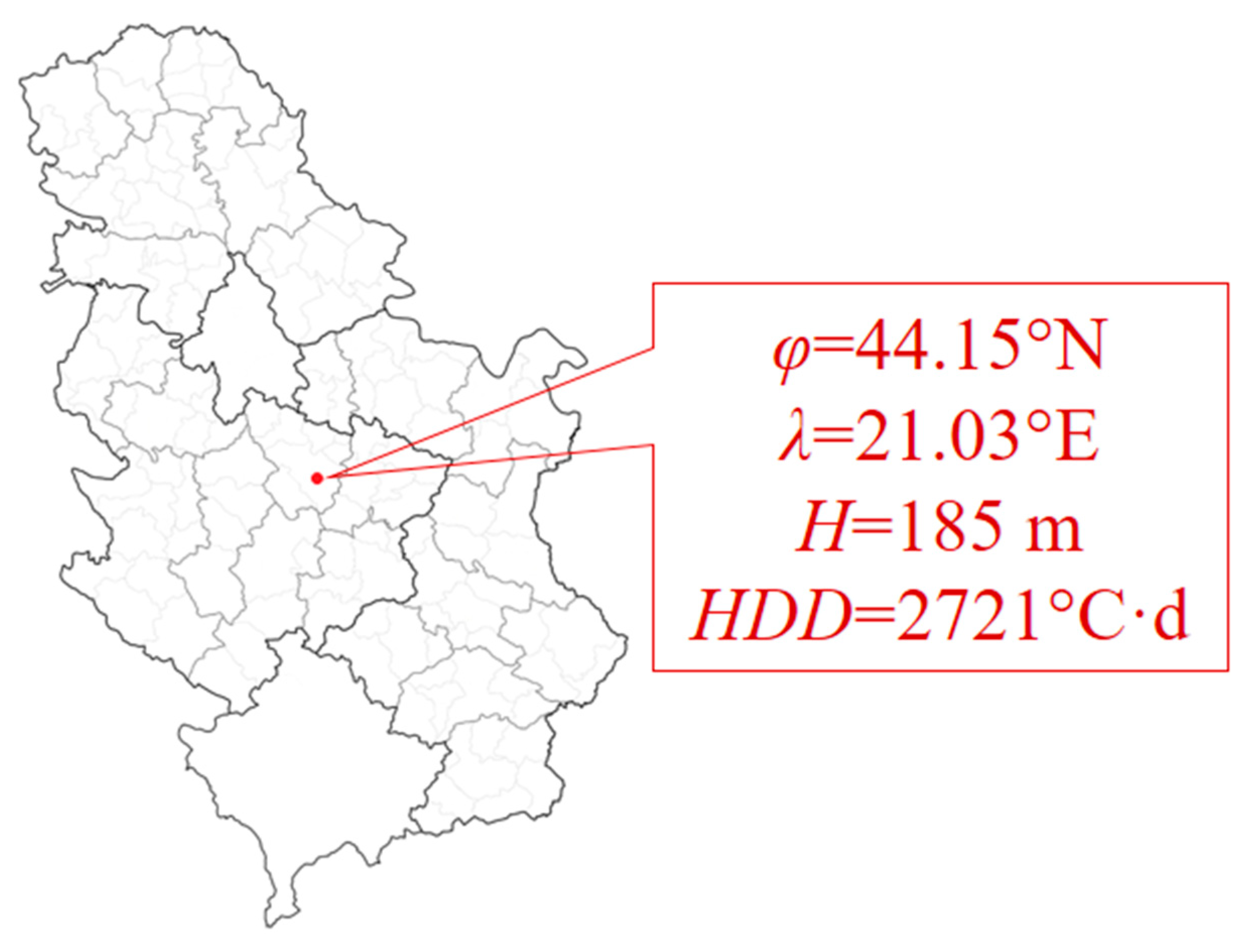
4. Location Parameters

4.1. Meteorological Data

Serbia (with time zone + 1 h) is a continental country in the Balkans. The climate is moderately continental (central and southern regions) and continental (northern regions), with distinct seasons. The summers are hot and humid. On the other hand, the winters are cold and snowy [63]. On the website Climate.OneBuilding.Org [64], meteorological data are available for a large number of cities in Serbia, including Kragujevac, i.e., KG (Figure 9).
During the analyzed 7-month period (from 1 October to 30 April), the average monthly temperature (Figure 10a) ranged between 0.39 °C (January) and 13.39 °C (October). The average monthly wind speed was higher than 2 m/s in November and February (Figure 10b). South and southwest winds were dominant under the influence of the Mediterranean climate (Figure 10c), with an attack angle between 200° and 250° (180° is for the south wind, and 270° is for the west wind).
During the analyzed 7-month period (from 1 October to 30 April), the average monthly temperature (Figure 10a) ranged between 0.39 °C (January) and 13.39 °C (October). The average monthly wind speed was higher than 2 m/s in November and February (Figure 10b). South and southwest winds are dominant—the influence of the Mediterranean climate (Figure 10c) because the attack angle is between 200° and 250° (180° is for the south wind, and 270° is for the west wind).
According to the data of Pavlović et al. [65] and Đurđević [66], the annual average solar irradiance on the horizontal (ground) surfaces is between 1250 kWh/m2 and 1450 kWh/m2, which is 154–354 kWh/m2 more than the European average (1096 kWh/m2). This indicator shows that the solar potential in central Serbia, i.e., Kragujevac, is underutilized; that is, there is a large potential for the additional installation of solar systems.
The individual components of incoming solar irradiance are weakest in intensity (Idir < 100 W/m2 and Idiff < 35 W/m2) in December and January (Figure 10d). Solar irradiance is strongest in April: Idir > 200 W/m2 and Idiff > 60 W/m2. The total incoming solar irradiance on the horizontal (ground) surface can also be determined using Figure 10d as the sum of direct and diffuse solar irradiance (Itot = Idir + Idiff [W/m2]).

4.2. Soil Temperature

The ceiling, i.e., the roof of the elevational ESB is located at a depth of 2 m from the free surface of the soil. Soil temperature at this depth, according to [67], can be determined by Equation (1):
t s , d = t s , a v g ( d = 0 ) t s , a m p ( d = 0 ) e d π 365 α s cos 2 π 365 d a y d a y min d 2 365 π α s
where ts,d [°C] is the average daily soil temperature during the year at depth d, ts,avg(d=0) [°C] is the average annual free soil surface temperature, ts,amp(d=0) [°C] is the temperature free soil surface amplitude, d [m] is the vertical distance from free soil surface to the ceiling (roof) of the elevational ESB, day [-] is the day of the year, daymin [-] is the phase constant corresponding to the day of minimum free soil surface temperature, and αs [m2/s] is the soil thermal diffusivity (for loam soil type αs = 0.91 × 10⁶ m2/s [68,69]).
Equation (1) does not take into account soil precipitation and soil heterogeneity properties at different locations and depths. The soil thermal diffusivity is based on prior knowledge of the soil density (ρs [kg/m3]), soil thermal conductivity (ks [W/(mK)]), and soil specific heat capacity (Cs [J/(kgK)]).
Average monthly soil temperatures at a depth of 2 m for Kragujevac are 12.61 °C (October), 11.73 °C (November), 10.29 °C (December), 9.58 °C (January), 11.07 °C (February), 12.34 °C (March), and 12.95 °C (April).

5. Numerical Analysis

5.1. Google SketchUp

Google SketchUp 8 software is intended for the 3D modeling of buildings and other objects [70]. The interface provides faster and simpler work compared to other CAD softwares CAD—Catia V5R20. Models with a large number of details can be created in this software. It also provides many other possibilities, such as integration with Google Earth services and EnergyPlus software (Legacy OpenStudio 1-0-11 (Legacy OpenStudio 1-0-11) and Legacy OpenStudio Rendering tool palettes). It also has a database with a large number of ready-made 3D models.

5.2. EnergyPlus

The EnergyPlus software is a useful tool for numerical investigations of energy flows in a building and its impact on the environment [71]. It was developed by Lawrence Berkeley, the National Laboratory, the US Army Construction Engineering Laboratory, and the University of Illinois [72]. The calculation algorithm uses the finite difference method (FDM). When combined with a large number of implemented mathematical models and appropriate weather files [64], different thermo-mechanical systems can be simulated (the calculation algorithm uses FDM): heating, cooling, air conditioning, ventilation, electrical devices, gas devices, solar systems, water supply, and sewerage, occupants, artificial lighting, etc.

5.3. Siemens Femap

Siemens Femap is a software application used for engineering numerical simulation and (structural and thermal) the analysis of objects, buildings, complex systems, plants, and production lines [73]. By using the FEM, it is possible to determine the degree of safety of constructions, their mechanical properties, and places with critical loads, from 1D beam models and thin-walled shell element modeling to 3D tet-dominant or hex-dominant meshing.

5.4. Scenario Simulation

5.4.1. EnergyPlus Preparations

The initial simulation model (Figure 2 and Figure 3), modeled according to the Rulebook on Energy Efficiency of New Buildings (Table 1), is an elevational ESB that passively uses geothermal (soil natural thermal insulation) and solar (the windows and the entrance door are positioned on the south facade wall) energy (Figure 11).
The elevational ESB is equipped with smart heating (GSHP, Figure 4) and lighting (AALCS, Table 2) thermo-technical systems. The thermal performance of the mentioned building was analyzed for 7 months (from 1 October to 30 April), depending on two variables (Figure 11): HOPVI type (first variable; three simulation models) and HOPVI depth (second variable; a total of 10 simulation models). The analyzed period (from 1 October to 30 April) includes the heating season (from 15 October to 15 April) and two transitional periods when there are sometimes needs for cooling and sometimes for heating, depending on the outside temperatures. The first transitional period lasts from 1 October to 14 October. The second transitional period lasts from 16 April to 30 April.
The first variable (HOPVI type; Figure 11) has already been mentioned (HOs performance—Section 3.1; PV performance—Section 3.2). The following figures show examples of elevation ESBs with different HOPVI types (for 2.5 m deep): type HO-1 (Figure 12), type HO-2 (Figure 13), and type HO-3 (Figure 14).
The second variable is very important. The depth of the HOPVI panels affects the energy (final and primary) consumption for heating and artificial lighting (with a negative direction), as well as electricity production (with a positive direction). Unlike other studies, in this case, the vertical supporting columns are taken into account. The number of and mutual distances depend on the depth of the HOs (Figure 15). Vertical supporting columns additionally influence the shading effects of an elevational ESB, so they must not be neglected.
All cases of combining the types and depths of the horizontal overhangs were analyzed separately with the appropriate simulation flows. In order to achieve the optimal depth for the horizontal overhangs, 31 simulation scenarios were conducted (one for the initial building model—without horizontal overhang—and 30 for the rest of the simulation scenarios).

5.4.2. Siemens Femap Preparations

A static structural analysis of all HOs in the HOPVI panel construction was performed within some boundary conditions (Figure 16).
The loads due to the PV panels are, on average, Fpv = 11 kg/m2 (field research of available PV panels on the local market). This value was used as one of the boundary conditions. According to recommendations in [74], the load due to snow (Fsn = 0.8 kN/m2) can be determined using Equation (2):
F s n = f s n K e x K t K o
where fsn [N/m2] is the specific load due to snow (fsn = 1 kN/m2), Kex [-] is the exposure coefficient (Kex = 1), Kt [-] is the thermal coefficient (Kt = 1), and Ko [-] is the overhang shape factor (Ko = 0.8).
The static structural analysis took into account the mass of the HOs (according to Table 3 and Figure 15), the mass of the PV panels, and the load due to snow cover for locations with a moderate continental climate.
The third component could have been neglected because of the continuous production of electricity from the PV panels during the analyzed period, which, in itself, implies that the HOPVI panels should always be cleaned, but this does not have to be a required practice.

5.5. Energy Balance

5.5.1. Final Energy Balance

Depending on the total final energy balance, each building can be classified into a certain BER (Figure 1). The same applies to elevational ESBs. For elevational ESBs to be in the EPB category (objective function) during the analyzed period (from 1 October to 30 April), the total final energy balance during this season must be negative (Ef,tot < 0 kWh), which is described by Equation (3):
E f , t o t = E f , t o t > 0   kWh E f , t o t = E f , t o t > 7175   kWh E S B N E E B 1537.5   kWh < E f , t o t 7175   kWh E S B L E B E f , t o t 1537.5   kWh E S B P B E f , t o t = 0   kWh E S B A B   or   Z E B E f , t o t < 0   kWh E S B E P B
where Ef,tot [kWh] is the total final energy balance in an elevational ESB during the analyzed period.

Final Energy Consumption

All energy flows in elevational ESBs are based on the use of electricity. In order to fulfill the condition Ef,tot < 0 kWh in Equation (3), electricity production must be greater than electricity consumption, as per Equation (4):
E f , t o t = E f , t o t , e = E f , t o t , e c o n s E f , t o t , e p r o d < 0   kWh
where Ef,tot,e [kWh] is the total final (electricity) balance, (Ef,tot,e)cons [kWh] is the total final (electricity) consumption (Equation (5)), and (Ef,tot,e)prod [kWh] is the total final (electricity) production.
E f , t o t , e c o n s = E f , t o t , e h + E f , t o t , e l + E f , t o t , e e q
where (Ef,tot,e)h [kWh] is the total electricity consumption for heating, (Ef,tot,e)l [kWh] is the total electricity consumption for lighting, and (Ef,tot,e)eq [kWh] is the total electricity consumption for electric equipment.

Heating System

Total electricity consumption for heating in Equation (6) is equal to the sum of electricity consumption for GSHP Egshp [kWh] in Equation (7), electricity consumption for circulation pump 1 (CP1) Ecp1 [kWh] (the primary heating connection between GSHP and GVPs), and electricity consumption for circulation pump 2 (CP2) Ecp2 [kWh] (the secondary heating connection between the GSHP and the FPHs):
E f , t o t , e h = E g s h p + E c p 1 + E c p 2
E g s h p = z = 1 7 E f p h z
where (Efph)z [kWh] is the electricity consumption for the FPH zone heater.

Lighting System

Since seven thermal zones (rooms) are equipped with SMLs (Table 2), then (Ef,tot,e)l is determined by Equation (8):
E f , t o t , e l = z = 1 7 E s m l z
where (Esml)z [kWh] is the electricity consumption for the SML zone lighting.

Final Energy Production

Total final (electricity) production in Equation (4) from HOPVI panels can be calculated as per Equation (9):
E f , t o t , e p r o d = E h o p v i = E p v = I s u n , t o t A p v S C p v η p v η i n v
where Ehopvi [kWh] is the electricity production from HOPVI, Epv [kWh] is the electricity production from PV panels, Isun,tot [kWh/m2] is the total solar irradiance incident on the PV panels, Apv [m2] is the area covered by the PV panels, SCpv [-] is the area fraction with active solar cells (SCpv = 0.85), ηpv [-] is the efficiency of the PV panels (ηpv = 0.2), and ηinv [-] is the efficiency of the DC/AC inverter (ηinv = 0.85).
Value Isun,tot (Figure 17) is determined by the following components in Equation (10):
I s u n , t o t = I s u n , d i r + I s u n , d i f f + I s u n , r e f l
where Isun,dir [kWh/m2] is the direct solar irradiance incident on the PV panels, Isun,diff [kWh/m2] is the diffuse solar irradiance incident on the PV panels in Equation (11), and Isun,refl [kWh/m2] is the reflected solar irradiance incident on the PV panels in Equation (12).
I s u n , d i f f = I s u n , d i f f , c r + I s u n , d i f f , s d + I s u n , d i f f , s h
I s u n , r e f l = I s u n , r e f , s + I s u n , r e f , o b
where Isun,diff,cr [kWh/m2] is the diffuse solar irradiance incident on the PV panels from the circumsolar region, Isun,diff,sd [kWh/m2] is the diffuse solar irradiance incident on the PV panels from the sky dome, Isun,diff,sh [kWh/m2] is the diffuse solar irradiance incident on the PV panels from the sky horizon, Isun,refl,s [kWh/m2] is the reflected solar irradiance incident on the PV panels from the soil, and Isun,refl,ob [kWh/m2] is the reflected solar irradiance incident on the PV panels from the obstacles.

5.5.2. Primary Energy Balance

Primary energy consumption, Ep,tot = Ep,tot,e [kWh], depends, in this case, on the primary energy transformation coefficient for electricity Rp,e [-]. If Rp,e = 2.5 [4], then Equation (13) holds:
E p , t o t = E p , t o t , e = E p , t o t , e c o n s E p , t o t , e p r o d = R p , e E f , t o t , e c o n s E f , t o t , e p r o d
where (Ep,tot,e)cons [kWh] in Equation (14) and (Ep,tot,e)prod [kWh] can be calculated for Equation (15):
E p , t o t , e c o n s = R p , e E f , t o t , e c o n s
E p , t o t , e p r o d = R p , e E f , t o t , e p r o d

5.5.3. Greenhouse Gases Balance

Analogously, Equation (13) for CO2 emission can be used to calculate Equation (16):
M c o 2 = M c o 2 , e = m c o 2 , e E p , t o t , e c o n s E p , t o t , e p r o d
where Mco2 = Mco2,e [kg] is the total CO2 emission, and mco2,e [kg/kWh] is the specific CO2 emission (mco2,e = 0.53 kg/kWh [4]).

5.5.4. Embodied Energy Balance

In order to determine the total embodied energy of HOPVI panels Eemb,tot = Eemb,hopvi [kWh] in Equation (17) during the exploitation period of 25 years (the adopted working life), the embodied energy for HO Eemb,ho [kWh] in Equation (18), and the embodied energy for PV panels Eemb,pv [kWh] in Equation (19) must be calculated separately, as per Equation (17):
E e m b , t o t = E e m b , h o p v i = E e m b , h o + E e m b , p v 25
E e m b , h o = wooden   support   columns + clay   tiles E e m b , h o 1 = E e m b , w s c + E e m b , c t steel   pipes + sheet   steel E e m b , h o 2 = E e m b , s p + E e m b , s s total   concrete   construction E e m b , h o 3 = E e m b , c c
E e m b , p v = e e m b , p v A p v
where Eemb,wsc [kWh] is the embodied energy for wooden support columns in Equation (20), Eemb,ct [kWh] is the embodied energy for clay tiles in Equation (21), Eemb,sp [kWh] is the embodied energy for steel pipes in Equation (22), Eemb,ss [kWh] is the embodied energy for sheet steel in Equation (23), Eemb,cc [kWh] is the embodied energy for concrete construction in Equation (24), and eemb,pv [kWh/m2] is the specific embodied energy for the PV panels (Table 3):
E e m b , w s c = e e m b , w s c ρ w s c V w s c
E e m b , c t = e e m b , c t ρ c t V c t
E e m b , s p = e e m b , s p ρ s p V s p
E e m b , s s = e e m b , s s ρ s s V s s
E e m b , c c = e e m b , c c ρ c c V c c
where (Table 3) eemb,wsc [kWh/kg] is the specific embodied energy for the wooden support columns, ρwsc [kg/m3] is the density for the wooden support columns, Vwsc [m3] is the volume of the wooden support columns, eemb,ct [kWh/kg] is the specific embodied energy for the clay tiles, ρct [kg/m3] is the density for the clay tiles, Vct [m3] is the volume for the clay tiles, eemb,sp [kWh/kg] is the specific embodied energy for the steel pipes, ρsp [kg/m3] is the density for the steel pipes, Vsp [m3] is the volume for the steel pipes, eemb,ss [kWh/kg] is the specific embodied energy for the sheet steel, ρss [kg/m3] is the density for the sheet steel, Vss [m3] is the volume for the sheet steel, eemb,cc [kWh/kg] is the specific embodied energy for the concrete construction, ρcc [kg/m3] is the density for the concrete construction, and Vcc [m3] is the volume for the concrete construction.

5.5.5. Total Energy Balance

In the end, the total energy balance Etot [kWh] is the sum of Ep,tot, and Eemb,tot, as per Equation (25):
E t o t = E p , t o t + E e m b , t o t

6. Results and Discussion

6.1. Static Structural Analysis

Analogous to Figure 6, Figure 7 and Figure 8, the following figures (Figure 18, Figure 19 and Figure 20) show characteristic displacement fields for the limiting case of depth (5 m) for all three HOPVI panel types: HO-1 (Figure 18), HO-2 (Figure 19), and HO-3 (Figure 20).
All HIOPV types (HO-1, HO-2, and HO-3), in addition to their weight, were tested for loads due to PV panels in snow conditions (Section 3.1). The results of the static calculations are shown in Table 4.
The maximum displacements (deformations) in the case of HO-1 (16.03 t, i.e., 157.25 kN) are 32.171 mm (Figure 18). The maximum displacements for HO-2 (11.4 t, i.e., 111.77 kN) amount to 34.619 mm (Figure 19). Finally, for HO-3, the maximum displacements are 3.4001 mm (38.6 t, i.e., 378.46 kN; Figure 20). In all analyzed cases, the degree of certainty is within the allowed limits (<0.7%): 32.171/5000 = 0.0064 (0.64%) for HO-1, 34.619/5000 = 0.0069 (0.69%) for HO-2, and 3.4001/5000 = 0.00068 (0.068%) for HO-3.

6.2. Final Energy Consumption

6.2.1. Heating System

The final (electricity) energy consumption for heating (GSHP) in the elevational ESB during the analyzed period (from 1 October to 30 April) for all scenarios (Figure 11 and Figure 15) is presented in Figure 21.
For the first type (HO-1, Figure 6 and Figure 12) of elevational ESB with HOPVI, electricity consumption for heating is (Figure 21) 1400.5 kWh (without HOPVI), 1419.66 (Dho-1 = 0.5 m), 1482.7 (Dho-1 = 1 m), 1797.69 (Dho-1 = 1.5 m), 1914.05 (Dho-1 = 2 m), 2023.84 (Dho-1 = 2.5 m), 2113.13 (Dho-1 = 3 m), 2173.23 (Dho-1 = 3.5 m), 2187.3 (Dho-1 = 4 m), 2205.43 (Dho-1 = 4.5 m), and 2215.18 (Dho-1 = 5 m).
Since the HO-1, HO-2, and HO-3 overhangs are characterized by an identical design for Dho = 0 m, Dho = 0.5 m, and Dho = 1 m (Figure 15), electricity consumption for the considered cases is the same (Figure 21): 1400.5 kWh (Dho-1 = Dho-2 = Dho-3 = 0 m), 1419.66 (Dho-1 = Dho-2 = Dho-3 = 0.5 m), and 1482.7 (Dho-1 = Dho-2 = Dho-3 = 1 m).
For other HO-2 depths, electricity consumption in the elevational ESB with HOPVI panels is (Figure 21) 1649.97 (Dho-2 = 1.5 m), 1780.91 (Dho-2 = 2 m), 1914.17 (Dho-2 = 2.5 m), 2012.88 (Dho-2 = 3 m), 2095.88 (Dho-2 = 3.5 m), 2128.12 (Dho-2 = 4 m), 2171.84 (Dho-2 = 4.5 m), and 2186.93 (Dho-2 = 5 m).
In the end, electricity consumption for the HO-3 type is (Figure 21) 1736.99 (Dho-3 = 1.5 m), 1846.42 (Dho-3 = 2 m), 1968.13 (Dho-3 = 2.5 m), 2056.03 (Dho-3 = 3 m), 2136.53 (Dho-3 = 3.5 m), 2164.95 (Dho-3 = 4 m), 2199.93 (Dho-3 = 4.5 m), and 2220.97 (Dho-3 = 5 m).
The biggest differences between the considered overhang types can be observed when Dho = 1.5 m. As the overhang surfaces increase with their depth, the differences decrease, so at a depth of 5 m, they are the smallest.
Figure 22 shows that the monthly electricity consumption for heating in elevational ESBs with HOPVI panels during the analyzed period is the highest in January (for all scenario simulations), from 381.07 kWh (Dho-1 = 0 m) to 502.52 kWh (Dho-1 = 5 m) for HO-1 (Figure 22a), from 381.07 kWh (Dho-2 = 0 m) to 496.61 kWh (Dho-2 = 5 m) for HO-2 (Figure 22b), and from 381.07 kWh (Dho-3 = 0 m) to 500.75 kWh (Dho-3 = 5 m) for HO-3 (Figure 22c).
On the other hand, electricity consumption is the lowest in October, from 20.41 kWh (Dho-1 = 0 m) to 129.35 kWh (Dho-1 = 5 m) for HO-1 (Figure 22a), from 20.41 kWh (Dho-2 = 0 m) to 126.71 kWh (Dho-2 = 5 m) for HO-2 (Figure 22b), and from 20.41 kWh (Dho-3 = 0 m) to 129.05 kWh (Dho-3 = 5 m) for HO-3 (Figure 22c).
Electricity consumption for circulation pumps (CPs) in elevational ESBs with HOPVI panels during the analyzed period for HO-1, HO-2, and HO-3 is presented in Figure 23.
For HO-1, circulation pumps consume between 20.28 kWh (without overhang) and 27.15 kWh (deep 5 m). The highest electricity consumption in the rest cases is 26.96 kWh (HO-2) and 27.24 kWh (HO-3), both for Dho = 5 m.
From the diagram in Figure 23, three characteristic zones can also be observed: the overlapping zone (0 m, 0.5 m, and 1 m), the zone of intense changes (1.5 m, 2 m, 2.5 m, and 3 m), and the zone of slow changes (3.5 m, 4 m, 4.5 m, and 5 m).
Electricity consumption for heating in an elevational ESB (Figure 21, Figure 22 and Figure 23) depends on solar gains (Figure 17). The shading effects increase with increasing overhang depth, and the solar gains are reduced, so the temperature of the free (southern) facade is lower. Figure 24 shows the daily (for 7 January) surface outside temperature for LR in an elevational ESB with HOPVI, depending on the type and dimension of the overhangs: HO-1 (Figure 24a), HO-2 (Figure 24b), and HO3 (Figure 24c).
Regardless of the HO types, the biggest temperature changes in the reference case (building without overhangs) can be observed in the period from 09:00 to 16:30. For example, at 12:45 pm, tlr,sr,out = 4.02 °C (for ESB without HOPVI). In the same period, this temperature is lower by 1.65 °C for Dho-1 = 5 m, 1.56 °C for Dho-2 = 5 m, and 1.61 °C for Dho-3 = 5 m.
Figure 24 also shows that in the early morning hours and late evening hours, the temperature of the south facade increases with the increase in the depth of the overhangs. This can be explained by the solar elevation angle (very small), so the diffuse and reflected components increase the total solar gains, following Equation (10).

6.2.2. Lighting System

Electricity consumption for the adopted lighting system (AALCS) in an elevational ESB with HOPVI panels during the analyzed period for HO-1, HO-2, and HO-3 is presented in Figure 25.
Regardless of HO types, AALCS electricity consumption is the same for Dho = 0 m (440.63 kWh), Dho = 0.5 m (441.31 kWh), and Dho = 1 m (443.79 kWh). The following discontinuities (drops in AALCS electricity consumption) can be seen in Figure 25: HO-1 (3 m, 3.5 m), HO-2 (3.5 m, 4 m), and HO-3 (3.5 m, 5 m). The discontinuities are explained by the different numbers, shapes, and dimensions of the vertical supporting columns (Figure 26—daily AALCS electricity consumption for LR: Figure 26a for HO-1, Figure 26b for HO-2, and Figure 26c for HO-3). The green line (Figure 25) shows the AALCS electricity consumption for different overhang depths in the variant without vertical columns (reference case). The highest AALCS electricity consumption is for Dho = 5 m: 560.22 kWh (HO-0), 607.63 kWh (HO-1), 582.33 kWh (HO-2), and 574.06 kWh (HO-3).

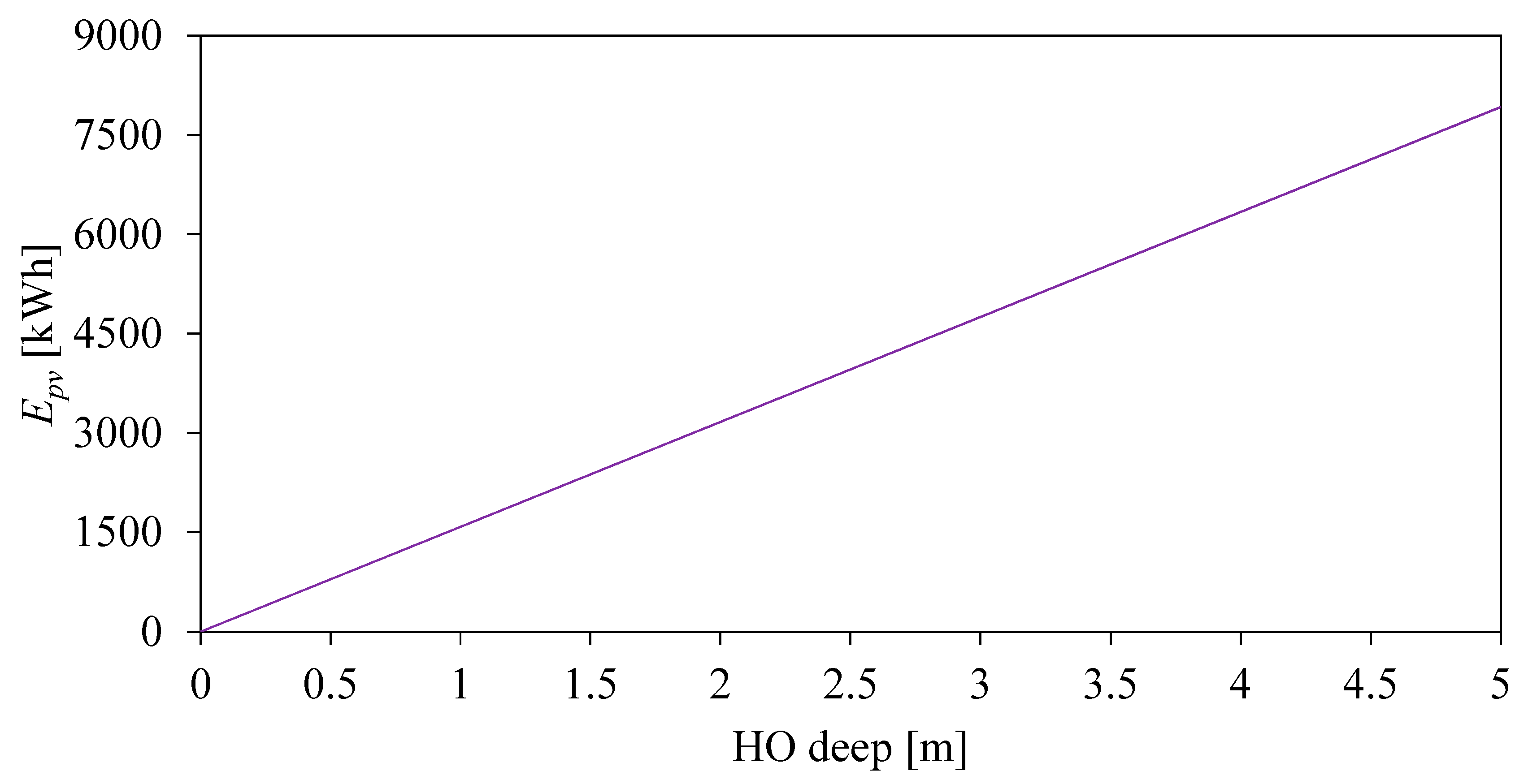
6.2.3. Electricity Production

All HOPVI panel types (HO-1, HO-2, and HO-3) are characterized by the same production of electricity (77.31 kWh/m2; Figure 27), which depends on the surface of the upper side of the overhangs, i.e., their depths: 792.44 kWh (Ahopvi = 10.25 m2), 1584.89 kWh (Ahopvi = 20.5 m2), 2377.33 kWh (Ahopvi = 30.75 m2), 3169.77 kWh (Ahopvi = 41 m2), 3962.22 kWh (Ahopvi = 51.25 m2), 4754.66 kWh (Ahopvi = 61.5 m2), 5547.1 kWh (Ahopvi = 71.75 m2), 6339.54 kWh (Ahopvi = 82 m2), 7131.99 kWh (Ahopvi = 92.25 m2), and 7924.43 kWh (Ahopvi = 102.5 m2).

6.3. Primary Energy Flow and Greenhouse Gas Emission

Considering the results shown in Figure 21, Figure 22, Figure 23, Figure 24, Figure 25, Figure 26 and Figure 27, as well as the corresponding Equations (13)–(16), the following diagram (Figure 28) shows the primary energy flows and CO2 emissions in an elevational ESB with HOPVI, depending on the overhang types with depth, as well as electricity consumption for water heating, electrical equipment, cooking, etc.
E f , t o t , a v g = E f , t o t , h o 1 + E f , t o t , h o 2 + E f , t o t , h o 3 3
E p , t o t , a v g = E p , t o t , h o 1 + E p , t o t , h o 2 + E p , t o t , h o 3 3
M c o 2 , a v g = M c o 2 , h o 1 + M c o 2 , h o 2 + M c o 2 , h o 3 3
One member of the household in Serbia consumes nearly 151.61 kWh/month of electricity [75] (for water heating, electrical equipment, cooking, etc.), which means that a family of four consumes 4245 kWh of electricity (final energy consumption) during 7 months (Figure 28a). The average primary energy consumption in an elevational ESB without HOPVI panels is 15,266.03 kWh (Equation (27)), and the CO2 emissions are 8090.99 kg (Equation (28)). A HOPVI panel system with Dho = 4.5 m provides EPB status because the primary energy consumption is between −141.9 kWh (for HO-1) and −297.575 kWh (for HO-2), while the CO2 emissions are between −75.21 kg (for HO-1) and −157.71 kg (for HO-2).
Figure 28b shows that the optimal dimension of the horizontal overhangs could be 4 m (average primary electricity consumption is −180.49 kWh, and the average CO2 emissions are −95.03 kg), with reduced electricity consumption for water heating, electrical equipment, cooking, etc., in an ESB with HOPVI panels on 3500 kWh.
Analogous to Figure 28a,b, the optimal dimension of the horizontal overhangs for an ESB with HOPVI panels could be 3.5 m if electricity consumption for additional needs is <3000 kWh (Figure 28c).
In the end, if the same indicator (people’s habits) reaches a value of 2500 kWh, the optimal depth of the overhang tends to reach a value of 3 m because the production of electrical energy that is delivered to the electrical network for Dho = 3 m is greater than the others (the average value is −922.86 kWh).

6.4. Embodied Energy and Total Energy Flow

The diagram in Figure 29 shows total embodied energy and total energy flow in an elevational ESB with HOPVI, depending on the overhang types and depths and electricity consumption for water heating, electrical equipment, cooking, etc.
Total embodied energy (Figure 29) is the lowest in the case of concrete HOPVI panels (HO-3). This applies to all analyzed cases. In second place are the steel HOPVI panels (HO-2), and HO-1 represents the most unfavorable type (from the point of view of embodied energy). The types and depths of the overhangs, in combination with the appropriate number of vertical support columns, caused the differences between HO-1 and HO-2 to be greater for depths ranging from 0 m to 1 m. For greater depths (1.5–5 m), these differences are much smaller, and a slight advantage is on the side of HO-2 (Figure 29).
When a comprehensive analysis of energy flows (the construction physics of the building, meteorological data, heating system, lighting system, people’s habits—electricity consumption 4245 kWh—and electricity production from PV panels) in an ESB with HOPVI panels is carried out while taking into account the final, embodied, and primary energy (for the adopted primary energy transformation coefficient for electricity; Rp,e = 2.5), the ESB with HOPVI panels is unable to reach EPB status (Figure 29a). Additionally, it can be concluded that an ESB with concrete HOPVI panels is the most favorable solution for reaching EPB status.
It can also be concluded that a reduction in electricity consumption to 3500 kWh provides EPB status for Dho = 5 m (the average total energy consumption for all overhang types is −805.82 kWh). A reduction in electricity consumption to 3000 kWh enables an ESB with HOPVI panels to reach the desired goal (goal function), even for 4.5 m deep horizontal overhangs (Etot = −409.16 kWh).
Interesting results are achieved when electricity consumption is reduced to 2500 kWh (89.29 kWh/month/person). Then the EPB status for all types of horizontal overhangs (HO-1, HO-2, and HO-3) is reached for Dho = 4.5 m (average total energy consumption is 1659.16 kWh) and also for Dho-3 = 4 m (Etot = −486.93, for HO-3). Precisely because the mentioned data values for the embodied energy for HO-3 are the smallest, a solution should be found for them.
However, when taking into account the trend of damaging the environment on a global level, as well as the current global political, economic, and social conditions, energy flows can no longer be viewed selfishly only from the human perspective (final energy consumption). The problem must be approached comprehensively, taking into account the reaction of the environment, which, despite a large number of legal norms, agreements, and other documents, is persistently ignored.

7. Conclusions

In this paper, the subject of the research is elevational earth-sheltered buildings with horizontal overhang photovoltaic-integrated panels. The authors combined a bioclimatic-passive construction approach, energy-efficient thermo-technical systems (ground source heat pump, geothermal vertical probes, floor panel heaters, circulation pumps, artificial and automatic lighting control systems, and PV panels), shading devices (three types of overhangs: wooden support columns covered with clay tiles, steel pipe support columns covered with sheet steel, and concrete support columns with concrete coverage) and the habits of tenants to determine the moment of reaching the energy-plus status regarding a building located in Kragujevac (Serbia); this was considered during the 7-month winter period (from 1 October to 30 April) because this time domain is very sensitive in terms of energy.
A static structural analysis was performed using the finite element method in the Siemens Femap software. Energy flow analysis was performed using the finite difference method in the EnergyPlus software (with the support of the Google SketchUp software).
The results showed that the energy-plus building status of such an architectural concept can be reached at a horizontal overhang depth of 3.5 m (for primary energy consumption) and 4.5 m (for total energy consumption). It was also concluded that the building energy rating of an ESB with HOPVI panels is greatly influenced by the habits of the ocupants, in addition to the construction physics of the building, meteorological data, heating system, lighting system, and electricity production from PV panels.
Modern architectural and construction design should not bypass such buildings, especially when taking into account the following facts: final energy consumption in the housing sector of the Republic of Serbia is still quite high, an increasing number of people live in cities, rural settlements are closing down, and the agricultural sector is collapsing.
The presented methodology can be applied to other locations in Europe and the world but with a very careful approach to assessing applicability. The specifics of climatic and geographical conditions, the specific production of electricity from PV panels, people’s habits, local differences in the field of energy efficiency in buildings, and other sensitive variables must be taken into account.

Author Contributions

Conceptualization, A.N., M.B. and R.K.; Methodology, A.N. and M.B.; Software, A.N. and M.B.; Validation, M.B.; Formal analysis, A.N., R.K., M.B. and A.J.; Investigation, A.N., R.K., M.B. and A.J.; Resources, R.K.; Data curation, R.K. and A.J.; Writing—original draft, A.N.; Writing—review & editing, A.N., R.K. and M.B.; Visualization, A.N.; Supervision, S.A.; Project administration, R.K., A.J. and S.A.; Funding acquisition, A.J. and S.A. All authors have read and agreed to the published version of the manuscript.

Funding

This research received no external funding.

Data Availability Statement

The original contributions presented in the study are included in the article, further inquiries can be directed to the corresponding author.

Conflicts of Interest

The authors declare no conflicts of interest.

Nomenclature

Symbols
AArea, [m2]
aDirection, [rad]
CSpecific heat, [J/(kgK)]
cSpeed, [m/s]
CHGConvective heat gains, [-]
COPCoefficient of performance, [-]
dDepth, [m]
dayDay of the year, [-]
EEnergy consumption (production), [J]
eSpecific energy, [J/kg]
FLoad, [N/m2]
fSpecific load, [N/m2]
FRFraction radiant, [-]
FVFraction visible, [-]
HElevation, [m]
HDDHeating degree days, [K·d]
ISolar irradiance, [W/m2]
KCoefficient, [-]
kThermal conductivity, [W/(mK)]
LSun illuminance, [lux]
lLength, [m]
MCO2 emission, [kg]
mSpecific CO2 emission, [kg/J]
nAir change, [l/h]
PPower, [W]
RPrimary energy transformation coefficient, [-]
RAFReturn air fraction, [-]
SCArea fraction with active solar cells, [-]
TAbsolute temperature, [K]
tTemperature, [°C]
UHeat transfer coefficient, [W/(m2K)]
VVolume, [m3]
WWidth, [m]
YmYoung’s Modulus, [Pa]
Greek letters
αThermal diffusivity, [m2/s]
ηEfficiency, [-]
λLongitude, [rad]
νPoisson ratio, [-]
ρDensity, [kg/m3]
φLatitude, [rad]
Indexes
aAir
adAdopted
ampAmplitude
avgAverage
ccConcrete construction
consConsumption
co2CO2 emission
cpCirculation pump
crCircumsolar region
ctClay tiles
dDeep
diffDiffuse
dirDirect
eElectric (electricity)
embEmbodied
eqElectric equipment
esbEarth-sheltered building
exExposure
fFinal
fphFloor panel heater
gfGround floor
gshpGround source heat pump
hHeating
hoHorizontal overhang
hopviHorizontal overhang photovoltaic-integrated panels
invInverter
lLight (lighting)
lrLiving room
maxMaximum
minMinimum
oOverhang
obObstacle
outOutside
pPrimary
prodProduction
pvPhotovoltaic panels
reflReflected
sSoil
sdSky dome
shSky horizon
smlSurface-mount light
snSnow
spSteel pipes
srSurface
ssSheet steel
sunSolar
tThermal
totTotal
wWind
wlWall
wscWooden support columns
wwWindow
zZone
Abbreviations
AALCSArtificial and automatic lighting control system
ABAutonomous building
ALArtificial lighting
BATBathroom
BDRBedroom
BERBuilding energy rating
CPCirculation pump
DLCSDay-lighting control system
EEBEnergy-efficient building
EPBEnergy-plus building
ESBEarth-sheltered building
FDMFinite difference method
FEMFinite element method
FPHFloor panel heater
GSHPGround source heat pump
GVPGeothermal vertical probes
HHall
HOHorizontal overhang
HOPVIHorizontal overhang photovoltaic-integrated panels
KKitchen
LEBLow-energy building
LRLiving room
NEEBNon-energy efficient building
PBPassive building
PVPhotovoltaic panels
SMLSurface-mount light
SRStorage room
WWRWindow–wall ratio
ZEBZero-energy building

References

  1. Ionescu, C.; Baracu, T.; Vlad, G.E.; Necula, H.; Badea, A. The historical evolution of the energy efficient buildings. Renew. Sustain. Energy Rev. 2015, 49, 243–253. [Google Scholar] [CrossRef]
  2. International Energy Agency. Available online: https://www.iea.org (accessed on 23 January 2024).
  3. Eurostat—European Commission. Available online: https://ec.europa.eu (accessed on 22 January 2024).
  4. Republic of Serbia—Ministry of Construction, Transport and Infrastructure. Available online: https://www.mgsi.gov.rs (accessed on 26 December 2023).
  5. Gupta, J.; Chakraborty, M. Energy efficiency in buildings. In Sustainable Fuel Technologies Handbook; Academic Press: Cambridge, MA, USA, 2021; pp. 457–480. [Google Scholar]
  6. Orman, Ł.J.; Majewski, G.; Radek, N.; Pietraszek, J. Analysis of thermal comfort in intelligent and traditional buildings. Energies 2022, 15, 6522. [Google Scholar] [CrossRef]
  7. Martin, R.; Arthur, T.; Jonathan, V.; Mathieu, T.; Enora, G.; Robin, G. SHAPE: A temporal optimization model for residential buildings retrofit to discuss policy objectives. Appl. Energy 2024, 361, 122936. [Google Scholar] [CrossRef]
  8. Dai, J.; Wang, J.; Bart, D.; Gao, W. The impact of building enclosure type and building orientation on indoor thermal comfort—A case study of Kashgar in China. Case Stud. Therm. Eng. 2023, 49, 103291. [Google Scholar] [CrossRef]
  9. Zheng, Z.; Xiao, J.; Yang, Y.; Xu, F.; Zhou, J.; Liu, H. Optimization of exterior wall insulation in office buildings based on wall orientation: Economic, energy and carbon saving potential in China. Energy 2024, 290, 130300. [Google Scholar] [CrossRef]
  10. Li, J.; Zheng, B.; Bedra, K.B.; Li, Z.; Chen, X. Effects of residential building height, density, and floor area ratios on indoor thermal environment in Singapore. J. Environ. Manag. 2022, 313, 114976. [Google Scholar] [CrossRef] [PubMed]
  11. Schorcht, M.; Jehling, M.; Krüger, T. Where are cities under pressure?—An indicator for measuring the impact of building changes on urban density. Ecol. Indic. 2023, 149, 110142. [Google Scholar] [CrossRef]
  12. Ge, J.; Wang, Y.; Zhou, D.; Gu, Z.; Meng, X. Effects of urban vegetation on microclimate and building energy demand in winter–An evaluation using coupled simulations. Sustain. Cities Soc. 2024, 102, 105199. [Google Scholar] [CrossRef]
  13. Kabore, A.; Ouellet-Plamondon, C.M. The impact of vegetable fibres on the shrinkage and mechanical properties of cob materials. Materials 2024, 17, 736. [Google Scholar] [CrossRef]
  14. Kalaimathy, K.; Priya, R.S.; Rajagopal, P.; Pradeepa, C.; Senthil, R. Daylight performance analysis of a residential building in a tropical climate. Energy Nexus 2023, 11, 100226. [Google Scholar] [CrossRef]
  15. Sepúlveda, A.; De Luca, F.; Thalfeldt, M.; Kurnitski, J. Analyzing the fulfillment of daylight and overheating requirements in residential and office buildings in Estonia. Build. Environ. 2020, 180, 107036. [Google Scholar] [CrossRef]
  16. Na, S.; Kim, S.; Moon, S. Additive manufacturing (3D Printing)-applied construction: Smart node system for an irregular building façade. J. Build. Eng. 2022, 56, 104743. [Google Scholar] [CrossRef]
  17. Sommese, F.; Badarnah, L.; Ausiello, G. Smart materials for biomimetic building envelopes: Current trends and potential applications. Renew. Sustain. Energy Rev. 2023, 188, 113847. [Google Scholar] [CrossRef]
  18. Raeissi, S.; Taheri, M. Optimum overhang dimensions for energy saving. Build. Environ. 1998, 33, 293–302. [Google Scholar] [CrossRef]
  19. Ossen, D.R.; Hamdan Ahmad, M.; Madros, N.H. Optimum overhang geometry for building energy saving in tropical climates. J. Asian Archit. Build. Eng. 2005, 4, 563–570. [Google Scholar] [CrossRef]
  20. Pacheco, R.; Ordóñez, J.; Martínez, G. Energy efficient design of building: A review. Renew. Sustain. Energy Rev. 2012, 16, 3559–3573. [Google Scholar] [CrossRef]
  21. Majewski, G.; Telejko, M.; Orman, Ł.J. Preliminary results of thermal comfort analysis in selected buildings. E3S Web Conf. 2017, 17, 00056. [Google Scholar] [CrossRef]
  22. Cho, J.; Yoo, C.; Kim, Y. Viability of exterior shading devices for high-rise residential buildings: Case study for cooling energy saving and economic feasibility analysis. Energy Build. 2014, 82, 771–785. [Google Scholar] [CrossRef]
  23. Valladares-Rendón, L.G.; Lo, S.L. Passive shading strategies to reduce outdoor insolation and indoor cooling loads by using overhang devices on a building. Build. Simul. 2014, 7, 671–681. [Google Scholar] [CrossRef]
  24. Bellia, L.; Marino, C.; Minichiello, F.; Pedace, A. An overview on solar shading systems for buildings. Energy Procedia 2014, 62, 309–317. [Google Scholar] [CrossRef]
  25. Park, J.; Choi, J.I.; Rhee, G.H. Enhanced single-sided ventilation with overhang in buildings. Energies 2016, 9, 122. [Google Scholar] [CrossRef]
  26. Nowak, H.; Nowak, L.; Sliwińska, E. The impact of different solar passive systems on energy saving in public buildings and occupants’ thermal and visual comfort. J. Build. Phys. 2016, 40, 177–197. [Google Scholar] [CrossRef]
  27. Sameti, M.; Jokar, M.A. Numerical modelling and optimization of the finite-length overhang for passive solar space heating. Intell. Build. Int. 2017, 9, 204–221. [Google Scholar] [CrossRef]
  28. Bojić, M.; Cvetković, D.; Bojić, L. Optimization of geometry of horizontal roof overhangs during a summer season. Energy Effic. 2017, 10, 41–54. [Google Scholar] [CrossRef]
  29. Valladares-Rendón, L.G.; Schmid, G.; Lo, S.L. Review on energy savings by solar control techniques and optimal building orientation for the strategic placement of façade shading systems. Energy Build. 2017, 140, 458–479. [Google Scholar] [CrossRef]
  30. Subhashini, S.; Thirumaran, K. A passive design solution to enhance thermal comfort in an educational building in the warm humid climatic zone of Madurai. J. Build. Eng. 2018, 18, 395–407. [Google Scholar] [CrossRef]
  31. Liu, S.; Kwok, Y.T.; Lau, K.K.L.; Chan, P.W.; Ng, E. Investigating the energy saving potential of applying shading panels on opaque façades: A case study for residential buildings in Hong Kong. Energy Build. 2019, 193, 78–91. [Google Scholar] [CrossRef]
  32. Rashid, M.; Malik, A.; Gulzar, S.; Jalil, A. The Efficacy of Shading Design in Commercial Buildings in the Semi-arid Climate of Lahore; Focusing on The Geometry of Horizontal Shade. Tech. J. 2019, 24, 1–10. [Google Scholar]
  33. Sghiouri, H.; Charai, M.; Mezrhab, A.; Karkri, M. Comparison of passive cooling techniques in reducing overheating of clay-straw building in semi-arid climate. Build. Simul. 2020, 13, 65–88. [Google Scholar] [CrossRef]
  34. Nikolić, D.; Đorđević, S.; Skerlić, J.; Radulović, J. Energy analyses of serbian buildings with horizontal overhangs: A case study. Energies 2020, 13, 4577. [Google Scholar] [CrossRef]
  35. Krarti, M. Evaluation of energy performance of dynamic overhang systems for US residential buildings. Energy Build. 2021, 234, 110699. [Google Scholar] [CrossRef]
  36. Krarti, M. Impact of PV integrated rotating overhangs for US residential buildings. Renew. Energy 2021, 174, 835–849. [Google Scholar] [CrossRef]
  37. Koç, S.G.; Kalfa, S.M. The effects of shading devices on office building energy performance in Mediterranean climate regions. J. Build. Eng. 2021, 44, 102653. [Google Scholar] [CrossRef]
  38. Mohammed, A.; Tariq, M.A.U.R.; Ng, A.W.M.; Zaheer, Z.; Sadeq, S.; Mohammed, M.; Mehdizadeh-Rad, H. Reducing the cooling loads of buildings using shading devices: A case study in Darwin. Sustainability 2020, 14, 3775. [Google Scholar] [CrossRef]
  39. Corti, P.; Bonomo, P.; Frontini, F. Paper review of external integrated systems as photovoltaic shading devices. Energies 2023, 16, 5542. [Google Scholar] [CrossRef]
  40. da Silva, F.T.; Veras, J.C.G. A design framework for a kinetic shading device system for building envelopes. Front. Archit. Res. 2023, 12, 837–854. [Google Scholar] [CrossRef]
  41. Kim, D.H.; Luong, H.T.; Nguyen, T.T. Optimizing the shading device configuration of kinetic façades through daylighting performance assessment. Buildings 2024, 14, 1038. [Google Scholar] [CrossRef]
  42. Jiang, Y.; Qi, Z.; Ran, S.; Ma, Q. A study on the effect of dynamic photovoltaic shading devices on energy consumption and daylighting of an office building. Buildings 2024, 14, 596. [Google Scholar] [CrossRef]
  43. Roy, R.L. Underground Houses: How to Build a Low-Cost Home; Sterling Publishing: New York, NY, USA, 1979. [Google Scholar]
  44. Akubue, J. Earth-sheltered housing; design concepts for urban ground-scrapers. Int. J. Archit. Arts Appl. 2021, 7, 1–7. [Google Scholar] [CrossRef]
  45. Zhu, X.; Liu, J.; Yang, L.; Hu, R. Energy performance of a new Yaodong dwelling, in the Loess Plateau of China. Energy Build. 2014, 70, 159–166. [Google Scholar] [CrossRef]
  46. Hassan, H.; El Kotory, A.M. A discussion of the application’s possibility of the earth-sheltered building type in Egypt: Implementation guidelines. Acad. Res. Community Publ. 2019, 3, 72–84. [Google Scholar] [CrossRef]
  47. Berezin, D.V. Earth-sheltering effect on dwelling in cold climate: Simulation-based and theoretical approaches. IOP Conf. Ser. Mater. Sci. Eng. 2019, 687, 055042. [Google Scholar] [CrossRef]
  48. Yadollahi, M.; Ali Shafaat, P.E.; Mohammadreza Hafezi, P.E. An algorithm for evaluating energy costs for earth-sheltered buildings. In ASHRAE Topical Conference Proceedings; American Society of Heating, Refrigeration and Air Conditioning Engineers, Inc.: Peachtree Corners, GA, USA, 2019; pp. 209–216. [Google Scholar]
  49. Callejas, I.J.A.; Apolonio, R.M.; Guarda, E.L.A.D.; Durante, L.C.; de Andrade Carvalho Rosseti, K.; Roseta, F.; Amarante, L.M.D. Bermed earth-sheltered wall for low-income house: Thermal and energy measure to face climate change in tropical region. Appl. Sci. 2021, 11, 420. [Google Scholar] [CrossRef]
  50. Khayami, S.; Ekhlassi, A.; Rahbar, M. Effect of earth-sheltering and atrium form and proportion integration on energy and lighting performance optimization in a hot arid climate of Mashhad, Iran. Energy Effic. 2023, 16, 6. [Google Scholar] [CrossRef]
  51. Rudnik, M.A.; Kurtović, F.N. Earth-sheltered housing buildings in the energy efficient structures context. Build. Mater. Struct. 2017, 60, 47–60. [Google Scholar]
  52. Milanović, A.R.; Kurtović Folić, N.; Folić, R. Earth-sheltered house: A case study of Dobraca village house near Kragujevac, Serbia. Sustainability 2018, 10, 3629. [Google Scholar] [CrossRef]
  53. Nešović, A.; Jurišević, N.; Kowalik, R.; Terzić, I. Potential of contemporary earth-sheltered buildings to achieve Plus Energy status in various European climates during the heating season. Build. Simul. 2023, 17, 41–52. [Google Scholar] [CrossRef]
  54. Nešović, A. Energy performance of infiltrated and elevational earth-sheltered buildings in the territory of the city of Kragujevac—A numerical investigation. Arhit. I Urban. 2023. [Google Scholar] [CrossRef]
  55. Rea, M.S. Lighting Handbook: Reference & Application, 8th ed.; Illuminating Engineering Society of North America: New York, NY, USA, 1993. [Google Scholar]
  56. Murata, K.; Kanazawa, T. Determination of Young’s modulus and shear modulus by means of deflection curves for wood beams obtained in static bending tests. Holzforschung 2007, 61, 589–594. [Google Scholar] [CrossRef]
  57. Mirmiran, A.; Wang, T.L.; Abishdid, C.; Huang, P.; Jiménez, D.L.; Younes, C. Performance of Tile Roofs under Hurricane Impact—Phase 2; Rep. No. SCL-070801; Department of Civil and Environmental Engineering, Florida International University: Miami, FL, USA, 2007. [Google Scholar]
  58. Hoque, M.E.; Noor, S.S.; Sultana, O.F. An Investigation of the Behavior of Mechanical Structures Due to Vibration Using ANSYS. In Proceedings of the International Conference on Mechanical Engineering and Renewable Energy, Chittagong, Bangladesh, 18–20 December 2017. [Google Scholar]
  59. Kamal, W.N.W.M.; Saad, N.H.; Ghani, A.R.A.; Abdullah, N.R.; Jazam, K.I.A. Modelling and simulation 1048 of a single deck bus subjected to rollover crash loading. Appl. Mech. Mater. 2013, 393, 453–459. [Google Scholar] [CrossRef]
  60. Al-Gabri, B.N.A.; Nabilah, A.B.; Aziz, F.A.; Karim, I.A. Numerical analysis of out-of-plane deformation of shear wall. IOP Conf. Ser. Earth Environ. Sci. 2019, 357, 012001. [Google Scholar] [CrossRef]
  61. Your Home—Australia’s Guide to Environmentally Sustainable Homes. Available online: https://www.yourhome.gov.au (accessed on 15 November 2023).
  62. Dale, M.; Benson, S.M. Energy balance of the global photovoltaic (PV) industry-is the PV industry a net 1053 electricity producer? Environ. Sci. Technol. 2013, 47, 3482–3489. [Google Scholar] [CrossRef] [PubMed]
  63. Republic of Serbia—Republic Hydrometeorological Service of Serbia. Available online: https://www.hidmet.gov.rs (accessed on 19 October 2023).
  64. Climate.OneBuilding.Org. Available online: https://climate.onebuilding.org (accessed on 18 October 2023).
  65. Pavlović, T.; Milosavljević, D.; Radonjić, I.; Pantić, L.; Radivojević, A.; Pavlović, M. Possibility of electricity generation using PV solar plants in Serbia. Renew. Sustain. Energy Rev. 2013, 20, 201–218. [Google Scholar] [CrossRef]
  66. Djurdjevic, D.Z. Perspectives and assessments of solar PV power engineering in the Republic of Serbia. Renew. Sustain. Energy Rev. 2011, 15, 2431–2446. [Google Scholar] [CrossRef]
  67. Van Dronkelaar, C.; Cóstola, D.; Mangkuto, R.A.; Hensen, J.L. Heating and cooling energy demand in underground buildings: Potential for saving in various climates and functions. Energy Build. 2014, 71, 129–136. [Google Scholar] [CrossRef]
  68. Joint Research Centre—European Soil Data Centre. Available online: https://esdac.jrc.ec.europa.eu (accessed on 28 November 2023).
  69. Andújar Márquez, J.M.; Martínez Bohórquez, M.Á.; Gómez Melgar, S. Ground thermal diffusivity calculation by direct soil temperature measurement. Application to very low enthalpy geothermal energy systems. Sensors 2016, 16, 306. [Google Scholar] [CrossRef]
  70. Google SketchUp Software. Available online: https://www.sketchup.com (accessed on 28 January 2024).
  71. EnergyPlus Software. Available online: https://energyplus.net (accessed on 20 January 2024).
  72. Crawley, D.B.; Lawrie, L.K.; Pedersen, C.O.; Winkelmann, F.C. Energy plus: Energy simulation program. ASHRAE J. 2000, 42, 49–56. [Google Scholar]
  73. Siemens Femap Software. Available online: https://plm.sw.siemens.com (accessed on 23 January 2024).
  74. Golubović, Z.; Simonović, M.; Mitrović, Z. Mechanics of Statics, 1st ed.; Faculty of Engineering University of Belgrade: Belgrade, Serbia, 2019. [Google Scholar]
  75. Republic of Serbia—Electricity Distribution of Serbia. Available online: https://elektrodistribucija.rs (accessed on 5 February 2024).
Figure 1. Interaction between EEB and BER in Serbia [4,5]: AB—autonomous building, EPB—energy-plus building, LEB—low-energy building, NEEB—non-energy-efficient building, PB—passive building, and ZEB—zero-energy building.
Energies 17 02100 g001
Figure 2. Research subject: ESB from LEB to EPB status.
Energies 17 02100 g002
Figure 3. Room arrangement in elevational ESB: BAT—bathroom, BDR1—bedroom 1, BDR2—bedroom 2, BDR3—bedroom 3, H—hall, K—kitchen, LR—living room, and SR—storage room.
Energies 17 02100 g003
Figure 4. Scheme of central heating system with a GSHP: FPH—floor panel heater, GSHP—ground source heat pump, HOPVI—horizontal overhang photovoltaic-integrated panels, GVP—geothermal vertical probes.
Energies 17 02100 g004
Figure 5. Reference point co-ordinates for LR.
Energies 17 02100 g005
Figure 6. Model HO-1 (wooden support columns covered with clay tiles).
Energies 17 02100 g006
Figure 7. Model HO-2 (steel pipe support columns covered with sheet steel).
Energies 17 02100 g007
Figure 8. Model HO-3 (concrete support columns with concrete coverage).
Energies 17 02100 g008
Figure 9. Geographical position of the city of Kragujevac.
Energies 17 02100 g009
Figure 10. Location parameters for the city of Kragujevac: (a) average monthly temperature, (b) wind speed, (c) wind direction, (d) solar irradiance (direct and diffuse) on the horizontal (ground) surfaces.
Energies 17 02100 g010
Figure 11. Considered cases.
Energies 17 02100 g011
Figure 12. Isometric view of elevational ESB with HOPVI panels (type HO-1 at a depth of 2.5 m deep).
Energies 17 02100 g012
Figure 13. Isometric view of elevational ESB with HOPVI panels (type HO-2 at a depth of 2.5 m).
Energies 17 02100 g013
Figure 14. Isometric view of elevational ESB with HOPVI panels (type HO-3 at a depth of 2.5 m).
Energies 17 02100 g014
Figure 15. All relations between HO types and HO depths.
Energies 17 02100 g015
Figure 16. Fixed support depending on the HO types and HO deeps. The first limitation refers to the fixing of vertical supporting columns in the ground (a). The second limitation refers to the fixing of the horizontal beam for the elevational ESB along its entire length (b). In some cases (HOs at a depth of 3 m), there are vertical supporting columns next to the elevational ESB itself (Figure 15), which are simultaneously fixed to the ground and the south facade wall of the building (c).
Energies 17 02100 g016
Figure 17. Solar irradiance model.
Energies 17 02100 g017
Figure 18. Displacement fields for HO-1.
Energies 17 02100 g018
Figure 19. Displacement fields for HO-2.
Energies 17 02100 g019
Figure 20. Displacement fields for HO-3.
Energies 17 02100 g020
Figure 21. GSHP electricity consumption in an elevational ESB with HOPVI panels (depending on the scenario simulation).
Energies 17 02100 g021
Figure 22. Monthly GSHP electricity consumption in an elevational ESB with HOPVI panels (depending on the scenario simulation): (a) HO-1, (b) HO-2, (c) HO-3.
Energies 17 02100 g022
Figure 23. CPS electricity consumption in an elevational ESB with HOPVI panels (depending on the scenario simulation).
Energies 17 02100 g023
Figure 24. Daily (7 January) LR surface outside temperature in an elevational ESB with HOPVI panels (depending on the scenario simulation): (a) HO-1, (b) HO-2, (c) HO-3.
Energies 17 02100 g024
Figure 25. AALCS electricity consumption in an elevational ESB with HOPVI panels (depending on the scenario simulation).
Energies 17 02100 g025
Figure 26. Daily (7 January) AALCS electricity consumption for LR in an elevational ESB with HOPVI panels (depending on the scenario simulation): (a) HO-1; (b) HO-2, (c) HO-3.
Energies 17 02100 g026
Figure 27. Electricity production in an elevational ESB with HOPVI.
Energies 17 02100 g027
Figure 28. Primary energy flow and CO2 emissions in an elevational ESB with HOPVI, depending on the overhang types and depth, electricity consumption for water heating, electrical equipment, cooking, etc.: (a) 4245 kWh, (b) 3500 kWh, (c) 3000 kWh, (d) 2500 kWh.
Energies 17 02100 g028
Figure 29. Total embodied energy and total energy flow in an elevational ESB with HOPVI, depending on the overhang types and depth and electricity consumption for water heating, electrical equipment, cooking, etc.: (a) 4245 kWh, (b) 3500 kWh, (c) 3000 kWh, (d) 2500 kWh.
Energies 17 02100 g029
Table 1. Heat transfer coefficients of construction elements.
Construction ElementUad [W/(m2K)]Umax [W/(m2K)]
Floor on the ground0.30.3
Exposed facade wall
Facade wall in the ground0.35
Flat roof above unheated space0.150.15
Flat roof above heated space0.3
Window1.51.5
Entrance door1.61.6
Table 2. Technical performances of SMLs.
Room (Zone)(Pe,l)z [W](Le,l)z [lux]RAF [-]FR [-]FV [-]CHG [-]
BDR12710000.720.180.1
BDR218
BDR3
BAT54700
K
LR36100
H1850
SRNo lighting system
Table 3. Mechanical and thermal performances of HO models.
Model HOHO-1HO-2HO-3
ConstructionSupporting ColumnsCoverSupporting ColumnsCoverSupporting
Columns
Cover
MaterialWoodClay titlesSteel pipesSheet steelConcrete
Ym,ho [GPa]12.513.7920021026.3
νho [-]0.550.20.30.2
ρho [kg/m3]700138478502400
eho,emb [MJ/kg]26.94.338.879.61.1
Source[56][57][58][59][60]
Table 4. Results of the static structural analysis.
GHO [kg]MaterialHO-1HO-2HO-3
Supporting
columns
Wood2875.60--
Steel pipes-1507.20-
Concrete--4492.8
CoverClay titles3667.60--
Sheet steel-400.35-
Concrete--24,600
PV panels1127.5
Snow8358.82
Total16,029.5211,393.8738,579.12
Disclaimer/Publisher’s Note: The statements, opinions and data contained in all publications are solely those of the individual author(s) and contributor(s) and not of MDPI and/or the editor(s). MDPI and/or the editor(s) disclaim responsibility for any injury to people or property resulting from any ideas, methods, instructions or products referred to in the content.

