The Balanced Energy Mix for Achieving Environmental and Economic Goals in the Long Run

Abstract

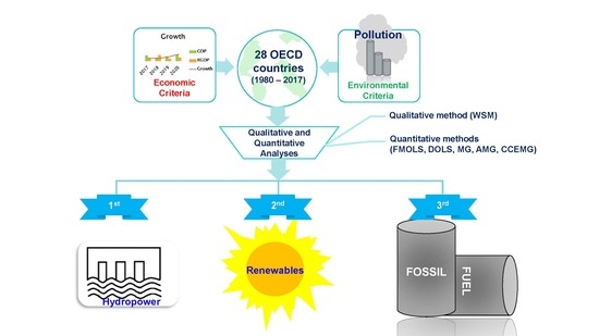
In this paper, we seek to find a balanced structure of energy sources that can simultaneously achieve two essential goals: (i) the environmental (degradation) goal and (ii) the economic (growth) goal. This study combines quantitative and qualitative methods to estimate and then rank each of the energy sources (including coal, gas, oil, hydropower, and renewable energy) to achieve the above two goals. This paper uses the weighted scoring method, the most popular method in multi-criteria decision-making techniques, to combine the rankings using five energy sources and two goals from panel data of 28 countries from Organization for Economic Co-operation and Development (OECD) countries for the period 1980–2017. Techniques for estimating the mean group long-run effect, including fully modified ordinary least squares (FMOLS) and dynamic ordinary least squares (DOLS), are used. The empirical findings of this paper reveal that, in the long term, in achieving both environmental goals and economic goals, the OECD countries should consider adopting a balanced energy mix in which the following structure is preferred: (i) hydropower, (ii) renewables and (iii) fossil fuels (oil, gas, coal).

1. Introduction

Energy is of widespread concern because of its effects on life, development, and the existence of current as well as future generations. Early in human history, fire was the primary energy source. Since then, we have exploited energy from various sources, such as coal, oil, hydropower, wind, solar, geothermal, and nuclear. Each source of energy has different advantages and disadvantages. In the past, fossil fuels were cheaper than renewables and had stable production. However, they caused pollution, whereas renewables were clean but limited in production. However, the selection of a source of energy depends on governmental direction, without deep and overall analysis of the economy and environment simultaneously.

Following the general trend of sustainable economic growth and development, which is generally known as green growth, the sustainable aspect of economic growth focuses on policies that can achieve economic growth not only for this generation, but also for many generations to come. The OECD countries have been formulating and implementing energy policies that are based on limiting CO₂ emissions by cutting and moving towards zero oil and coal use. The energy use of the United Kingdom has been transferred dramatically from fossil to clean energies, which accounted for 52 percent of the total energy consumption in 2017 [1]. In the US, the current government is still interested in fossil fuels. However, the government is planning to switch to solar and wind because of its low cost and environmentally friendly attributes. However, the US economy is still heavily dependent on fossil energy, particularly coal and oil. Limiting the use of fossil fuels will reduce the amount of CO₂ released into the environment, but at the same time, slow down economic growth [2].

Some countries take advantage of their natural advantages to develop and exploit renewable energy. In Sweden, renewable energy (mainly wind, nuclear and hydro) accounts for a share of more than half of the domestic demand. This current level is expected to increase further by 100 percent by 2040 [1]. The most significant problem for energy policies with a focus on renewable energy is the guarantee of energy security for the nation.

On the other hand, the problem with oil-use countries is the fluctuations in oil prices. We note that oil prices are unpredictable and uncontrollable, especially in the event of unexpected events like the COVID-19 pandemic. The impact of oil prices on the consumer price index (CPI) in these countries is very significant, requiring quick actions from the government in seeking alternative energy sources or supporting the economy with stimulus packages. The need to balance sustainable economic growth and development and environmental protection should be a top priority in energy policy.

In general, energy policies are based on various factors, including internal and external factors, such as price stabilization, reducing CO₂ emissions and ensuring energy security, affordability, and suitability to the economy. However, decisions are mainly based on specific information for each factor, without considering the balance of economics and the environment simultaneously. As such, we consider that this paper will provide an additional piece of empirical evidence for governments to consider when they formulate and implement energy mix policies in their countries.

The empirical papers on energy economics to date appear to focus on the investigation of a relationship among variables of interest. For example, empirical studies on the environmental Kuznets curve hypothesis (EKC), a highly cited concept in energy economics studies, generally focus on the three main streams of analyses. The first stream empirically examines the change in the traditional EKC theory. The second stream investigates the nexus between environmental quality and total energy use. The last stream of research investigates the inter-relationship between trade openness, proxied by foreign investment flows, and environmental quality.

This paper is unique and different from other empirical papers in the area of energy economics and policy implications. In this paper, we seek to find a balanced structure of energy sources that can simultaneously achieve important goals in both domains: (i) the environment and (ii) the economy. Advanced countries such as Japan, the United Kingdom and France (and many others) have been advancing towards the use of cleaner energy sources to minimize the negative impacts of energy consumption on environmental degradation. The governments of developing and emerging countries appear to prioritize economic growth and development. The debate about striking the right balance between what we call the environmental goal and the economic goal appears to have been ignored in the current literature.

The structure of this paper is as follows: Section 2 discusses selected empirical studies on energy economics to date, with a focus on the three strands of research in response to the environmental Kuznets curve hypothesis. Section 3 presents the research methodology and data. The empirical findings of this paper, including the sensitivity analyses, are included in Section 4, followed by the conclusions in Section 5 of the paper.

2. Literature Review

This paper is based on two traditional theories/hypotheses, including the Kuznets environment curve from environmental studies and economic growth theory. For the first hypothesis, in the 1950s, Simon Kuznets examined the relationship between economic growth and initial inequality. The Kuznets curve hypothesis states that when a nation follows industrialization, especially in agricultural mechanization, the economic center of a nation will move gradually towards the urban zones. The consequence of this development is that farmers and unskilled laborers from rural areas have to change their workplace by moving to large cities in order to earn more. This movement causes a substantial gap in earnings between people living in rural areas and downtown areas. Business owners earn profits. Workers in these industries receive an increase in income at a slower rate. However, the incomes of farmers fall because the population in rural areas declines, while the urban population increases. Nevertheless, inequality then declines as economic growth reaches the highest level of average income. An increase in Gross Domestic Product (GDP) per capita follows after the country reaches the optimal level of industrialization. Kuznets states that this inequality tends to resemble a U-shaped curve, where it increases first and then decreases with the increase in GDP per capita.

After decades of hypothesizing, Kruger and Grossman [3] apply the concept to their research in the field of the environment. Kuznets’ curve is used to illustrate the relationship between economic growth and environmental degradation. An inverted U-shaped correlation is found. These results indicate that the nation’s early stage of economic growth can be associated with the sacrifice of environmental quality. This view supports observations from developing and emerging countries. However, when a relatively high level of economic growth and development is achieved, the concerns for environmental quality emerge and increase. As a result, the inverted U-shape of the EKC curve has been supported by various empirical studies, including Shafik [4] and Omotor and Orubu [5]. This relationship has been considered a standard feature in engineering for formulating and implementing environmental policies. Onafowora and Owoye [6] indicate the long-term relationship between economic development and CO₂ emissions. Al-Mulali and Oxturk [7] also confirm the U-shaped relationship between GDP and CO₂ emissions.

Given the importance of the concept, may empirical studies have been conducted to examine the validity of the EKC hypothesis. In the beginning, time series analyses with many different techniques are employed such as Auto Regressive Distributed Lag (ARDL), Vector Auto Regression (VAR), the Vector Error Correction Model (VECM), and Granger causality to investigate the nexus of economic growth and environmental quality for specific countries or groups of countries. Empirical papers to date appear to focus on the investigation of a relationship among variables of interest using panel data. Mixed results on this relationship are reported, including studies from Ang [8], Hossain [9], Lean and Smyth [10], Magazzino [11], and Magazzino [12]. In particular, Rahman and Velayutham [13] confirm no causal relationship or unidirectional causality in the short and long run. In contrast, Zhang [14], Shahbaz et al. [15], Salahuddin et al. [16] report on the bidirectional relationship between economic growth and environmental quality. Niu et al. [17] indicate the unidirectional causality findings in the short run, and the directional relationship is observed in the long run.

In addition to testing the validity of traditional EKC theory (the inverted U-shape curve), a new stream of research examines whether a so-called N-shaped relationship between income and CO₂ emissions does exist. This stream of research has raised many empirical research questions, which have been explored by various scholars such as Rahman and Velayutha [13], To et al. [18], Sarkodie and Strezov [19], Churchill et al. [20], Zhou et al. [21], Magazzino [22], and Magazzino [14]. Churchill et al. [20] test the N-shape relationship for the OECD countries in the period 1870–2014 using mean group estimators (Mean Group (MG), Pooled Mean Group (PMG), Augmented Mean Group (AMG), and Common Correlated Effects Mean Group (CCEMG)). They find two turning points in terms of GDP per capita, i.e., the relationship exhibits an N-shape in some countries such as Australia, Canada, and Japan, but not in others, such as Spain and the UK. Moreover, Sarkodie and Strezov [19] also test this N-shape in the top five developing countries that emit a significant level of greenhouse gases, including China, Iran, Indonesia, India, and South Africa, using panel quantile regression with data from 1982 to 2016. The findings of this study confirm the N-shaped relationship between per capita income and CO₂ emissions in selected countries, leading to support for the validity of the EKC hypothesis.

In addition, unlike other papers, the second background theory utilized in this paper is based on economic growth theory. Economic growth has been considered an important and interesting topic for many economists. Barro [23], who supplements the classical and neoclassical growth models, studies the growth model, which considers additional variables of energy and other macro variables, including the impact of government on economic growth in the long run. This model simultaneously tests the validity of Keynes’ theory and provides evidence on an unclear relationship between economic growth and environmental quality. By assuming government spending is complementary to private-sector production, Barro’s model points to the non-monotonous relationship between government spending and economic growth. Hence, the neoclassical growth model with the participation of government such as the model of Barro [23] is often used in the research to test the factors affecting economic growth [24].

Empirical research based on growth theory and the growth model of Barro [23] conducts two main empirical tests. The first empirical test examines the impact of the government’s role on economic development. The second test examines the link between economic growth and energy consumption, a stream that normally runs alongside EKC research.

The mechanism and level of the economic impact of public spending remain controversial and are explained by different theories. In Keynesian economics, economic output is determined by aggregate demand. Meanwhile, along with factors such as consumption, income, and net exports, public spending is seen as an important derivative of aggregate demand [25]. Consequently, therefore, Keynes argued that government involvement in the economy is necessary. When the economy is in recession, the government needs to maintain demand for investment to stimulate private investment with large public investment programs, also known as the “crowding-in effects” hypothesis of public spending with private investment [26,27].

In contrast, neoclassical growth models argue for the “crowding-out effects” of public spending on private investment [28,29,30,31,32]. Government spending can directly substitute private investment, thereby slowing future growth [31]. Furthermore, government demand for goods and services may cause interest rates to rise. As a result, capital becomes more expensive, negatively affecting access to private sector capital. By raising taxes or borrowing to finance public spending, public spending also makes it difficult for the private sector to access scarce financial resources [30,31].

Many economists, such as Devarajan et al. [33], Chen [34], and Ghosh and Gregoriou [35], extended Barro’s model to examine the impact of different components of government spending on economic growth. By assigning different elasticity coefficients to different sectors of government expenditure, their models can determine the optimal scale and structure of the public sector for economic growth.

The empirical findings of other papers confirm the negative effect of public spending on economic growth [36,37]. In contrast, a positive contribution of public spending to economic growth has also been found in other studies [38]. Meanwhile, a few studies have found public spending to have non-linear effects on economic growth [39]. Interpreting the results of a mixed test, Gemmell et al. [24] point out the role of budget constraints in the relationship between public spending and economic growth. Nevertheless, empirical studies examining the role of budget constraints in the relationship between public spending and economic growth are quite limited [24,40].

In other words, empirical studies that test the relationship between energy consumption and economic growth face problems with inconsistency and conflicting results among researchers. In the beginning, researchers found a one-directional effect of this nexus; however, the direction between them is actually the opposite. For instance, Soytas and Sari [41] find no bidirectional nexus between the two, while Lee [42] confirms a causal relationship in which energy consumption affects economic growth and vice versa.

Huang et al. [43]; To et al. [18]; Vo et al. [44] state the reasons for their inconsistent results: (1) the difference in the period of the time series; (2) the use of time series techniques without analyzing or controlling for structural change (change in the short run) and the business cycle; (3) the sample period not being long enough to analyze the long-run effects. Thus, to address these issues, especially the disadvantages of time series data, To et al. [18] used macro panel data (panel data with a large time dimension) on 25 emerging and developing countries to determine the causality nexus between energy consumption, foreign direct investment (FDI), CO₂ emissions, and GDP. They found an inverted N-shaped relationship between GDP and environmental degradation. An inverted U-shaped nexus between FDI and CO₂ emissions is also found in these emerging and developing countries, which implies a trade-off between economic growth and the quality of the environment, in which environmental standards are relaxed to attract more foreign investment. Moreover, they also stated the positive impact of energy consumption on CO₂ emissions. This finding is consistent with the results of Chandran and Tang [45] and Acaravci and Ozturk [46].

In this paper, the authors simultaneously use the EKC hypothesis on the environment and Barro’s economic growth model. Unlike previous papers, our study does not utilize energy consumption as the total amount of energy. In contrast, our study breaks down energy consumption into various energy sources. We then carefully analyze the impact of each energy source on the environment and economic growth. This analysis is done together with the use of macroeconomic panel data to estimate the long-run effect for each energy source. Based on the estimated coefficients, all energy sources are ranked in order of those that are the least harmful to the environment and that provide the most significant contribution to economic growth. We believe that the approach which was taken for solving our research objective is new. Multi-criteria decision making (MCDM) analyses, including five energy sources and two criteria, are considered to combine these two rankings from two criteria (environmental degradation and economic growth). This study uses the weighted scoring method (WSM), the most popular method for MCDM [47,48,49], to score all rankings from five sources and two criteria. This method chooses a set of several alternatives (energy sources), which depend on the score for each alternative and the weighting for each criterion. The final optimal structure of energy sources is a set of five sources that satisfy the two most important criteria, including: (i) the most positive and significant effect on economic growth, and (ii) the least harmful effect on the environment by reducing CO₂ emissions.

3. Methodology and Data

3.1. Models Representing for the Environmental Goal and the Economic Goal

To determine an energy structure that simultaneously achieves both the environmental degradation goal and the economic growth goal, we construct a model including two distinct parts for achieving these two goals simultaneously: (i) the environmental degradation goal and (ii) the economic growth goal.

-

The first part, with a focus on the environmental goal, ranks five energy sources based on the level of CO₂ emissions.

-

The second part, with a focus on the economic goal, ranks five energy sources (coal, gas, oil, hydropower, and renewable energy) based on their impact on economic growth.

To combine the rankings from these two parts, we develop a multi-criterion decision-making technique (MCDM) using five energy sources (including coal, gas, oil, hydropower, and renewable energy) and two criteria (environmental goal and economic goal). The weighted score method (WSM), the most popular method in MCDM [47,48,49], is used to score all the ranking results. The final structure for the energy mix demonstrates a source of energy (coal, gas, oil, hydropower, and renewable energy) in the order of preferences that satisfy the following two conditions: (i) a particular source of energy does the least harm to the environment or has the lowest CO₂ emissions and (ii) a particular source of energy boosts economic growth the most.

3.1.1. The Environmental Goal

The rankings related to the environmental goal are employed following an examination of the validity of the traditional EKC hypothesis [50]. The non-linear relationships between environmental quality and income are reported. More specifically, the relationship has an inverted U-shape, which means that, after a threshold level of income, an increase in income will reduce the negative effect on environmental quality. On this basis, the model takes the following form [18]:

EQ = f(GDP, GDP², EC)

where EQ stands for the environment quality, which can be proxied by the level of emissions, such as CO₂. In order to raise the reliability of the analysis and estimation, the proxy variable should have a long time period. As such, we consider that employing CO₂ emissions as the proxy is appropriate. Income and square income are widely used in empirical analyses testing a non-linear relationship between economic growth and environmental degradation. EC stands for energy consumption, which comprises the consumption of five energy sources: oil, gas, coal, hydropower, and renewable energy. Employing various energy sources allows us to separate the contribution of each energy source to environmental quality. With these variables, we construct a regression model, model 1, as follows:

CO_{2 it} = π₀ + π₁GDP_it+ π₂GDP²_it + π₃Coa_it+ π₄Gas_it+ π₅Oil_it + π₆Hyd_it + π₇Ren_it + ε_it

(1)

where carbon emissions (CO₂) are used as the dependent variable.

Various independent variables are used, including per capita real GDP, per capita real GDP squared and cubed, and per capita consumption of coal, gas, oil, hydropower, and renewable energy. All variables are transformed into their logarithmic form.

3.1.2. The Economic Growth Goal

According to growth theories, empirical studies on testing and estimating the effect of growth factors are commonly based on the production function, especially the Cobb-Douglas [51] function, divided into four main factors: technology, capital, human resources, and natural resources. These empirical studies normally transform the model into a logarithmic form to facilitate analysis. The output growth model of Barro [52] is basically presented as follows:

∆Y = F(Y, Y*)

where ∆Y is the growth rate of income/output, Y is per capita income/output, and Y* is the long-run level of income/output or potential income/output of an economy. The value of Y* is based on government policies such as investment in education, research activities, and increases in capital. ∆Y is positively related to Y* and negatively related to Y. The Barro model, which includes control variables, is as follows:

∆Y_it = π₀ + π₁Y_{o i} + π₂∆EC_it+ π₃X_it+ ε_it

where ∆Y_it is the economic growth rate of country i at year t, Y_{o I} stands for the logarithm of initial per capita GDP of country i, and EC_it denotes the log of energy consumption of country i at year t. Barro [52] and Huang et al. [43] used control variables (X_it), including inflation, capital stock, government spending, growth of labor, and degree of international openness. Model 2 is written as follows:

∆lnY_it = π₀ + π₁lnY_{o i} + π₂∆lnCoa_it+ π₃∆lnGas_it+ π₄∆lnOil_it + π₅∆lnHyd_it + π₆∆lnRen_it +π₇INF_it + π₈CAP_it + π₉GEX_it + π₁₀∆lnLF_it + π₁₁TRADE_it + ε_it

(2)

where:

∆lnY_it: the first difference in the logarithm of per capita income for the country i at year t;

lnY_{o i}: the log of initial per capita income of country i;

∆lnCoa/Gas/Oil/Hyd/Ren_it: the first difference in the logarithm of coal, natural gas, oil, hydropower, and renewable energy consumption for country i at year t;

INF_it: inflation rate of country i at year t;

CAP_it: gross fixed capital formation for country i at year t (%GDP);

GEX_it: general government final consumption expenditure for country i at year t (%GDP);

∆lnLF_it: the first difference in the logarithm of the labor force for country i at year t;

TRADE_it: total export and import as a share of GDP for country i at year t (%GDP).

3.2. Econometric Techniques

Two models, model 1 representing the environmental goal and model 2 representing the economic goal, are analyzed using the same econometric techniques. Various econometric analyses, including the cross-sectional test, the stationary test, and panel cointegration test, are conducted. Nguyen and Vo [53] and To et al. [18] state that this procedure can be estimated by three steps. First, macro panel data have a long time dimension; thus, the first step for the macro panel data is the same as with the time series data. Second, the order of integration for each variable of the macro panel data needs to be tested and determined. Third, a prerequisite for the existence of a long-run relationship is the presence of cointegration between variables. Once cointegration is confirmed, the long-run relationship between the group of integrated variables can be investigated using the Vector Error Correction Model (VECM) (see [54,55]). These tests are discussed in detail by To et al. [18].

If these tests are verified, and the results show that there is at least one long-run nexus between explanatory variables and the dependent variable, then the long-run estimators are employed. The most popular models for estimating the mean group long-run effect, which can treat endogeneity problems and serial correlation in macro panel data, are fully modified ordinary least squares (FMOLS) and dynamic ordinary least squares (DOLS). These techniques, FMOLS and DOLS, are used in this paper. The purpose of this study is to find a balanced structure of energy sources (coal, gas, oil, hydropower, and renewable energy). As such, after conducting regressions, these five energy sources are ranked based on their regressors.

-

For the first criterion (with a focus on the environmental degradation goal, using the model of EKC as presented in Equation (1)), the first priority is the source of energy that has the smallest effect on environmental degradation or the smallest regression coefficient obtained in model 1. As such, these five sources of energy are ranked based on the magnitude of their respective regressors, in the following order: (i) negative impact on CO₂ emissions or negative coefficients (statistically significant); (ii) no impact (zero coefficients with statistically significant) or the coefficients are statistically insignificant; (iii) positive coefficient (statistically significant).

-

For the second criterion (with a focus on the economic growth goal, using the growth model as presented in Equation (2)), the first priority is the source of energy that has the largest contribution to economic growth. As such, the following order is used to rank energy sources: (i) statistically significant with a positive sign, (ii) no impact (zero coefficient with insignificant coefficient), and (iii) negative contribution (statistically significant).

3.3. Weighted Scoring Method

The weighted scoring method (WSM) is then used in the next step to combine the two sets of rankings (one set for the environmental goal and the other set for the economic goal) based on the score for each of the five energy sources (coal, gas, oil, hydropower, and renewable energy). The following equation is used:

S(A_i) = ∑W_j x S_ij.

The multi-criteria decision-making techniques (MCDM) in this paper now consist of two criteria {C₁, C₂} (being the environmental criterion and the economic criterion) and five energy sources {A₁, A₂, A₃, A₄, A₅} (being coal, gas, oil, hydropower, and renewable energy) in a decision matrix of all choices {S_ij}, where {S_ij} is the score after calculating and evaluating the performance of choices using criterion {C_j}. The weights {W₁, W₂} indicate the importance or the role of a specific criterion. A sensitivity analyses using different sets of weights are also conducted to ensure the robustness of the findings.

3.4. Data

Data are used for both model 1 (on the environmental goal) as presented in Equation (1) and model 2 (on the environmental goal) as presented in Equation (2). Data are collected for the period from 1980 to 2017 for 28 developed countries in the Organization for Economic Co-operation and Development (OECD), which include the following countries: Australia, Austria, Belgium, Canada, Chile, Czech Republic, Denmark, Estonia, Finland, France, Germany, Greece, Hungary, Iceland, Ireland, Israel, Italy, Japan, Korea, Rep., Latvia, Lithuania, Luxembourg, Mexico, Netherlands, New Zealand, Norway, Poland, Portugal, Slovak Republic, Slovenia, Spain, Sweden, Switzerland, Turkey, United Kingdom, and the United States.

The description of all variables in both model 1 and model 2 are presented in

Table 1. Definitions of the variables.

Variable	Measurement	Definition	Source
Carbon emissions (CO2)	Metric tons per capita	CO2 emissions are generated by burning fossil fuels and by consumption of solid, liquid and gas fuel, and gas.	International Energy Agency *
Per capita income (GDP)	GDP per capita (current US$)	GDP per capita is the ratio between the gross domestic product and the midyear population	WDI, World Bank
Oil consumption (Oil)	Tons of per capita oil equivalent)	Crude oil is an unrefined oil, and it is classified as fossil fuels. It includes hydrocarbon residues and other organic materials. It can be refined to produce usable products such as gasoline, diesel, petrochemicals (such as plastics), fertilizers, and even drugs.	BP Statistical Review of World Energy **
Gas consumption (Gas)	Consumption of natural gas (tons of oil equivalent per capita)	Natural gas is a fossil fuel that is a mixture of combustible gases, including most of the hydrocarbons.	BP Statistical Review
Coal consumption (Coa)	Consumption of coal (tons of oil equivalent per capita)	Coal consumption is commercial coal, which is primarily used as a solid fuel for electricity generation and combustion.	BP Statistical Review
Hydropower consumption (Hyd)	Consumption of hydropower (tons of oil equivalent per capita)	Hydropower consumption, based on total primary hydropower output, does not account for transboundary electricity supply. Consumption is converted from energy generation data, with an assumption of efficiency of 38% based on data from modern thermal power plants	BP Statistical Review
Renewable energy consumption (Ren)	Consumption of Renewable energy (tons of oil equivalent per capita)	Renewable energy consumption, based on the total output from renewable sources, including wind, geothermal, solar, biomass, and waste, and does not account for cross-border power supplies	BP Statistical Review
Inflation rate (INF)	Based on consumer prices (annual %)	Inflation represents an increase in the general price of goods and services over time in the economy.	World Bank
Gross fixed capital formation (CAP)	Measured by dividing investment by income (%)	Total fixed capital includes improvements in land, factories, machines, vehicles, weapons, intellectual property, rare assets (gold, silver and others), underground assets (oil, coal and others), and other natural assets.	World Bank
Government expenditure (GEX)	Measured by dividing public spending by income (annual %)	General government expenditure includes all current government spending on the purchase of goods and services (excluding military spending)	World Bank
Labor force (LF)	Total labor force	The labor force includes all people who are of working age who have a job or are looking for work.	World Bank
International openness (TRADE)	Measured as % of GDP	It is calculated by dividing the sum of exports and imports by GDP.	World Bank

* CO₂ emissions are affected by burning data from fossil fuels, soil, and cement equipment, collected by the Carbon Dioxide Information Analysis Center (CD CDIAC). The center collected global carbon dioxide emissions between 1950 and 1982, estimated by Marland and Rotty [56] from fuel production data from the UN’s Energy Statistics Yearbook [57]. We consider that the main reason for the use of fuel production data is due to a higher level of reliability in comparison with fuel consumption data at the global level. This choice of using fuel production data is widely utilized in empirical analyses. Moreover, doing so will also avoid creating an accounting identity in Equation (1). We consider that when energy consumption data is used, the total of estimated coefficients for GDP, GDP² in Equation (1) is equal to zero. ** Collected from government sources and published data, including data from the Energy Research of the Institute of Geosciences and Natural Resources which is available in BP Statistical Review [58].

.

Table 2. Descriptive statistics.

Variable *	Mean	Standard Error	Skewness	Kurtosis	Min	Max	Obs.
CO2 (log)	2.11	0.53	−0.36	3.34	0.50	3.44	1064
GDP (log)	9.91	0.86	−0.80	3.52	7.13	11.69	1064
GDP2 (log)	98.95	16.55	−0.55	3.08	50.81	136.63	1064
Coal consumption (log)	5.56	1.88	−2.03	6.97	−1.38	8.52	1064
Natural gas consumption (log)	5.56	2.18	−1.67	4.84	−0.89	7.91	991
Oil consumption (log)	0.54	0.49	−0.70	4.39	−1.07	1.93	1064
Hydropower consumption (log)	4.33	2.75	−0.53	2.63	−2.90	9.15	1054
Renewable energy consumption ** (log)	−11.92	7.60	0.06	2.80	−34.79	9.51	986
Inflation	7.67	20.91	9.73	137.60	−4.48	373.22	1064
Capital formation	22.81	3.92	0.67	4.33	11.54	39.40	1064
Government expenditure	18.55	4.61	−0.02	3.12	7.52	38.24	1064
Labor force (dlog)	0.01	0.02	4.33	53.78	−0.05	0.25	961
Trade openness	73.56	49.04	3.11	16.95	16.01	416.39	1064

* The unit production data is a million tonnes of oil equivalent (Mtoe). ** Renewable energy includes biomass, geothermal, solar, wind, and other renewable sources.

presents the descriptive statistics of the variables utilized in our two models.

4. Empirical Results

4.1. Test of Presence of Cross-Sectional Dependence

The first step in the regression technique is to test for the presence of cross-sectional dependence, and the results from this test affect all the techniques used in the subsequent steps. As a result, to obtain strong test results, we use three simultaneous tests: Pesaran [59], Friedman [60], and Frees [61]. Although the three tests have their advantages and disadvantages, they also provide an overview of the robustness of the results. Moreover, two of the specifications (fixed effect and random effect) are employed in the three tests in both models to reveal the change in the test results.

If the null hypothesis is accepted, there is no cross-sectional dependence, and the appropriate unit root test for all data is the Pesaran test [62]—the second generation of panel unit root tests, and the long-run estimator methods are pooled using FMOLS and DOLS [18]. In contrast, all the results in

Table 3. Sectional independence tests.

	Pesaran		Friedman		Frees
	CD Test	p-Value	CD	p-Value	CD (Q)	p-Value
Model 1: Environment
FE model	2.089 **	0.0367	42.632 **	0.0211	3.949 ***	0.000
RE model	2.173 **	0.0298	46.507 ***	0.0080	4.130 ***	0.000
Model 2: Economic
FE model	50.617 ***	0.000	230.101 ***	0.000	8.563 ***	0.000
RE model	47.956 ***	0.000	228.886 ***	0.000	8.499 ***	0.000

Notes: Fixed effects (FE) and random effects (RE) models. *** and ** indicate statistical significance at the one and five percent level, respectively.

, including six tests for each model, strongly reject the null hypothesis at the one percent and five percent significance levels. That means that all data samples have cross-sectional dependence or are sample country specific. This leads to a change in the test used in the following steps. In this case, the unit root test used should be the one by Im, Pesaran, and Shin (IPS test; [63]), which is expanded in the Choi test for cross-sectional dependence. Furthermore, mean group regressions, such as main mean group analysis, including fully modified ordinary least squares (FMOLS), dynamic ordinary least squares (DOLS) and the other mean group analysis methods, including Mean Group (MG), Common Correlated Effects Mean Group (CCEMG) and Augmented Mean Group (AMG), should be used to determine the long-run effects [64].

4.2. Panel Unit Root Tests

A unit root test is conducted to determine the stationarity and the integration of the same order for variables used in the paper [18]. This test is required before the cointegration tests are conducted to examine the long-run nexus between CO₂ emissions and each source of energy (model 1) and economic growth and each source of energy (model 2). The results of the unit root tests and robustness checks are presented in

Table 4. Unit root test using Pesaran test.

Variables	Level		First Difference		Order of Integration
	Constant	Constant and Trend	Constant	Constant and Trend
lnCO2	0.969	−0.672	−16.158	−15.002	I(1)
	(0.834)	(0.251)	(0.000)	(0.000)
lnGDP	−0.11	−0.103	−13.964	−11.918	I(1)
	(0.456)	(0.459)	(0.000)	(0.000)
lnGDP2	0.034	0.014	−13.602	−11.442	I(1)
	(0.514)	(0.506)	(0.000)	(0.000)
lncoa	2.032	2.407	−13.365	−11.547	I(1)
	(0.979)	(0.992)	(0.000)	(0.000)
lngas	0.661	3.816	−12.924	−12.06	I(1)
	(0.746)	(1.000)	(0.000)	(0.000)
lnoil	3.495	−1.203	−14.358	−12.208	I(1)
	(1.000)	(0.114)	(0.000)	(0.000)
lnhyd	−0.651	−1.037	−19.948	−18.359	I(1)
	(0.258)	(0.150)	(0.000)	(0.000)
lnren	−0.237	−0.403	−12.499	−10.724	I(1)
	(0.406)	(0.344)	(0.000)	(0.000)
INFCPI	−1.911	−0.171	−14.968	−13.106	I(1)
	(0.028)	(0.432)	(0.000)	(0.000)
CAP	−0.281	1.351	−13.002	−10.442	I(1)
	(0.389)	(0.912)	(0.000)	(0.000)
GEX	−0.863	1.154	−9.131	−7.272	I(1)
	(0.194)	(0.876)	(0.000)	(0.000)
lnLF	0.922	0.260	−6.546	−5.563	I(1)
	(0.822)	(0.603)	(0.000)	(0.000)
TRADE	−1.171	0.190	−12.965	−10.474	I(1)
	(0.121)	(0.575)	(0.000)	(0.000)

Standard errors in parentheses.

below. The robustness checks from all four tests are presented for all variables, with the constant and the trend and constant shown in both the level and first difference forms.

4.3. Panel Cointegration Test Results

Cointegration tests, including those by Kao [65], Pedroni [66], and Westerlund [67], are employed after confirming the stationarity at the same order I(1) in Table 4. This step helps to avoid spurious results [18], and we conduct these three tests at the same time to obtain robust results. All the results are in

Table 5. Cointegration tests for model 1 (Equation (1)).

	Test Statistic	p-Value
Kao test for cointegration
Modified Dickey–Fuller t	−2.6220 ***	0.0044
Dickey–Fuller t	−1.1550	0.1239
Augmented Dickey–Fuller t	−0.3082	0.3790
Unadjusted modified Dickey–Fuller t	−3.1510 ***	0.0008
Unadjusted Dickey–Fuller t	−1.4200 *	0.0778
Pedroni test for cointegration
Modified Phillips–Perron t	2.3250 ***	0.0100
Phillips–Perron t	−4.1450 ***	0.0000
Augmented Dickey–Fuller t	−4.0770 ***	0.0000
Westerlund test for cointegration
Variance ratio	−2.3404 **	0.0333

Notes: ***, **, and * show the rejection of the null hypothesis of no cointegration is statistically significant at the 1, 5, and 10 percent levels, respectively.

and

Table 6. Cointegration tests for model 2 (Equation (2)).

	Test Statistic	p-Value
Kao test for cointegration
Modified Dickey–Fuller t	−28.5952 ***	0.0000
Dickey–Fuller t	−18.8550 ***	0.0000
Augmented Dickey–Fuller t	−16.9937 ***	0.0000
Unadjusted modified Dickey–Fuller t	−34.1630 ***	0.0000
Unadjusted Dickey–Fuller t	−19.3050 ***	0.0000
Pedroni test for cointegration
Modified Phillips–Perron t	−2.2520 **	0.0122
Phillips–Perron t	−8.6760 ***	0.0000
Augmented Dickey–Fuller t	−8.4680 ***	0.0000
Westerlund test for cointegration
Variance ratio	−2.0190 **	0.0218

Notes: *** and ** show the rejection of the null hypothesis of no cointegration is statistically significant at the 1, 5, percent levels, respectively.

.

In Table 5, the result is highly statistically significant at one percent in both the Kao and Pedroni tests and at five percent in the Westerlund test using model 1, a model of the environment. We conclude that some or all panels show cointegration between variables. In other words, there may be at least one long-run nexus between the variables in model 1. Therefore, the use of Panel Vector Auto Regression (P-VAR), which is used for evaluating the short-run effect, is not considered in this research.

Similarly, the growth model for the environment has the same results in the cointegration test. All the results, which are in Table 6, reject the null hypothesis at a highly significant level (one percent). This critical step ensures that at least one variable in model 2 has a long-run relationship with the dependent variable (economic growth rate). Overall methods, both models 1 and 2 show robustness in their test results, which predict high reliability in conclusion to this study.

4.4. Regression and Ranking Results

We consider that ordinary least squares (OLS) regression is inappropriate, leading to a biasedness in estimating the long-run equilibrium relationship. In this paper, we apply fully modified ordinary least squares (FMOLS) in order to take the endogeneity problems, as well as the serial correlation issues, into account [68,69]. In addition, dynamic ordinary least squares (DOLS) is also employed, as this DOLS technique can also eliminate endogeneity problems and serial correlation issues using contemporaneous values, leads, and lags in the first difference. Due to the greater use of assumptions and the reduction in the degrees of freedom by using leads and lags [70,71], FMOLS is the preferred model in this study. However, we use the result of the DOLS model to confirm the direction of the estimated coefficients.

4.4.1. Model 1: Environmental Goal

We employ the traditional model of the environment (Kuznet [50]) with the control variables (income and square of income) and the proxy variable for energy consumption, which is divided into five main sources of energy (coal, gas, oil, hydropower, and renewable energy) that have enough data for analysis. Furthermore, in this model, the multicollinearity problem between GDP and sources of energy is very clear in the variables in model 2 (the impact of energy use on the growth rate). To analyze the effect of the multicollinearity problem on the coefficient of the variables of concern, we use both models (FMOLS and DOLS) and other mean group models with and without control variables (GDP and GDP²). The regression results are shown in

Table 7. Regression results for model 1 (dependent variable: lnCO₂).

Variable	Rank	Main Mean Group Models		Other Mean Group Methods
		FMOLS	DOLS	MG	CCEMG	AMG
Coal	4	0.273 ***	0.273 ***	0.225 ***	0.245 ***	0.232 ***
		(0.007)	(0.004)	(0.025)	(0.025)	(0.021)
Gas	3	0.166 ***	0.190 ***	0.136 ***	0.135 ***	0.123 ***
		(0.012)	(0.008)	(0.021)	(0.021)	(0.021)
Oil	5	0.533 ***	0.522 ***	0.585 ***	0.560 ***	0.591 ***
		(0.013)	(0.007)	(0.036)	(0.036)	(0.031)
Hydropower	1	−0.0073 *	−0.0134 ***	−0.0186 ***	−0.012 **	−0.0151 **
		(0.004)	(0.002)	(0.007)	(0.006)	(0.008)
Renewable	2	−0.0001	−0.0001 ***	−0.0000	−0.0005	0.0001
		(0.000)	(0.000)	(0.000)	(0.001)	(0.001)
GDP		0.0013	−0.0785	−0.0454	−0.086	0.112
		(0.107)	(0.079)	(0.268)	(0.248)	(0.260)
GDP2		−0.0011	0.0026	0.0024	0.0061	−0.0055
		(0.005)	(0.004)	(0.013)	(0.012)	(0.013)
Constant		2.191 ***	2.596 ***	2.136	3.146 ***	1.3900
		(0.540)	(0.399)	(1.390)	(1.196)	(1.340)
Observation		912	912	912	912	912

Standard errors in parentheses, *** p < 0.01, ** p < 0.05, * p < 0.1.

and

Table 8. Robustness check for model 1 by excluding the income variables.

Variable	Rank	Main Mean Group Models		Other Mean Group Methods
		FMOLS	DOLS	MG	CCEMG	AMG
Coal	4	0.255 ***	0.253 ***	0.229 ***	0.242 ***	0.254 ***
		(0.009)	(0.014)	(0.023)	(0.024)	(0.027)
Gas	3	0.152 ***	0.174 ***	0.140 ***	0.113 ***	0.120 ***
		(0.020)	(0.035)	(0.024)	(0.021)	(0.020)
Oil	5	0.595 ***	0.586 ***	0.558 ***	0.547 ***	0.552 ***
		(0.024)	(0.035)	(0.040)	(0.033)	(0.038)
Hydropower	1	0.0275 ***	0.0204 **	−0.0177 ***	−0.0147 **	−0.0095
		(0.005)	(0.010)	(0.006)	(0.007)	(0.007)
Renewable	2	−0.0003 *	−0.0007	−0.0002	−0.0002	0.0002
		(0.000)	(0.000)	(0.000)	(0.000)	(0.001)
Constant		2.078 ***	2.058 ***	1.937 ***	0.765 **	1.987 ***
		(0.030)	(0.050)	(0.068)	(0.380)	(0.062)
Observation		912	912	912	912	912

Standard errors in parentheses, *** p < 0.01, ** p < 0.05, * p < 0.1. All variables are transferred into logarithmic form. Note: A rank of one denotes the least environmental harm, and a rank of five denotes the most environmental harm.

.

This step aims to determine the impact of energy sources on environmental degradation before we do any further rankings. The main concern is how the coefficient or final rankings of these sources change across multicollinearity problems and multiple specifications. If there is no difference or the deviation in regressors between specifications is small, or the statistical significance is still high, the final rank based on these coefficients is the most reliable.

With these concerns in mind, the first considerations in the results in both Table 7 and Table 8 are the sign and magnitude of the estimated coefficients for all five energies (coal, gas, oil, hydropower, and renewable energy). In the main models, FMOLS and DOLS with and without a multicollinearity check, the coefficient of coal consumption is from +0.253 to +0.273. This deviation is quite low and highly significant (one percent). This coefficient means that when coal consumption increases/decreases by one percent, on average, CO₂ emissions increase/decrease by 0.273 percent (FMOLS model), ceteris paribus. The coefficient for gas consumption is from +0.152 to +0.19, and all regressors are also highly statistically significant (at one percent). The economic meaning is similar to that for coal consumption, in that a change in the use of gas of one percent leads to a 0.17 percent change in CO₂ emissions (in the same direction). Oil and hydropower consumption have high statistical significance as well, but oil use has the biggest effect on CO₂ emissions (a one percent increase/reduce in oil use, on average, leads to a 0.53 percent increase/decrease in CO₂ emissions). In contrast, the effect of renewable energy is unclear and has a weak significance. These results indicate no evidence that the use of renewables leads to environmental degradation.

Based on the magnitude and signs of the regressors, the following steps are used to rank the five energy sources: (1) a negative impact on CO₂ emissions or a negative coefficient (statistically significant); (2) no impact (zero coefficient with statistically significant) or the coefficient is statistically insignificant; (3) positive coefficient (statistically significant). The final rank is as follows: hydropower, renewable energy, gas, coal and oil in the order of the least environmental harm to the most environmental harm, as indicated in Table 8.

4.4.2. Model 2: Economic Goal

This step considers the impact of each energy source on economic growth in the long run by applying Barro’s growth model. In accordance with the approach adopted for the environmental model (Equation (1)), this analysis for the economic growth model (Equation (2)) also uses the five mean group methods, FMOLS, DOLS, MG, CCEMG and AMG, to regress the effects. The results are presented in

Table 9. Regression and ranking results.

∆lnGDP	Rank	Main Mean Group Models			Other Mean Group Methods
		FMOLS	DOLS	MG	CCEMG	AMG
lnGDP0		−0.0132 ***		0.000	0.000	0.000
		(0.005)		0.000	0.000	0.000
∆lncoa	5	−0.0483 *	−0.0219	0.0017	−0.0537	0.0114
		(0.029)	(0.014)	(0.050)	(0.064)	(0.039)
∆lngas	2	0.112 ***	0.125 ***	−0.0661	−0.0442	0.001
		(0.036)	(0.021)	(0.075)	(0.081)	(0.053)
∆lnoil	1	0.548 ***	0.176 ***	0.577 ***	0.0153	0.419 ***
		(0.064)	(0.049)	(0.119)	(0.125)	(0.098)
∆lnhyd	3	0.0158 *	0.0184 ***	0.0152	0.0819 *	0.0265
		(0.009)	(0.004)	(0.024)	(0.044)	(0.017)
∆lnren	4	−0.0014 ***	−0.0009 ***	−0.0016	−0.0116	−0.0044
		(0.000)	(0.000)	(0.004)	(0.009)	(0.004)
INFCPI		0.0093 ***	0.0043 ***	0.0054 *	−0.0015	−0.0047 *
		(0.001)	(0.000)	(0.003)	(0.005)	(0.003)
CAP		0.0047 ***	0.0101 ***	−0.0079 **	−0.0044	−0.004
		(0.001)	(0.001)	(0.004)	(0.005)	(0.004)
GEX		0.0014	−0.0003	−0.0313 ***	−0.0621 ***	−0.0530 ***
		(0.002)	(0.001)	(0.007)	(0.017)	(0.006)
dlnLF		0.332	−1.437 ***	0.671 *	−1.187	0.152
		(0.306)	(0.202)	(0.385)	(0.863)	(0.292)
TRADE		0.0007 *	−0.0016 ***	−0.0016 **	0.0000	−0.004 ***
		(0.000)	(0.000)	(0.001)	(0.002)	(0.001)
Constant		0.0000	−0.130 ***	0.900 ***	−18.03	1.508 ***
		0.000	(0.013)	(0.191)	(14.380)	(0.186)
R2		0.739	0.945

Standard errors in parentheses, *** p < 0.01, ** p < 0.05, * p < 0.1. Note: A rank of one denotes the most contribution to economic growth, and a rank of five denotes the least contribution to economic growth.

.

4.5. A Combination of These Two Criteria Using the Weighted Scoring Method

We then use the weighted scoring method (WSM) to obtain a score for the five sources, in which the order of these scores shows their final contribution to the balanced structure of energy sources (including coal, gas, oil, hydropower, and renewable energy). The most preferred source of energy is the energy source with the highest score. In this method, the weight of each criterion plays an important role in the score and directly affects the final ranking. Thus, to obtain an overview of the final rank and its role in achieving both environmental and economic goals, we analyze changes in the final rank across the two scenarios step by step with sensitivity analyses. Using the weights of each criterion range from 70% to 80%,

Table 10. Final ranking for each of the energy sources.

Source *	Model 1 (Environment Goal)	Model 2 (Economic Goal)	Weighting Range **		Final Ranking ***
			Environment Scenario	Economic Scenario	Environment Scenario	Economic Scenario
Coal	4	5	70% to 80%	70% to 80%	5	5
Gas	3	2			3	2
Oil	5	1			4	1
Hydro	1	3			1	3
Renew	2	4			2	4

* Hydro stands for hydropower, and Renew stands for other types of renewable energy, including wind, geothermal, solar, biomass, and waste. ** With the environmental scenario, the weighting of the environmental goal ranges from 70% to 80% and the remaining proportion of 20–30% applies to the economic goal. The same approach applies to the economic scenario, with a weight of 70–80%, leaving 20–30% for the environmental goal. *** The final ranking takes into account the rankings from estimated coefficients from models 1 and 2, together with the assumed weighting range. Robustness analyses are presented in the Appendix A of this paper. Note: A rank of one denotes the most contribution to economic growth, and a rank of five denotes the least contribution to economic growth. A rank of one denotes the least environmental harm, and a rank of five denotes the most environmental harm.

shows how the WSM method works and the influence of this weight on the final structure.

In the environmental goal scenario, we assume that a government prioritizes the environmental goal rather than the economic goal. We assign scores for each energy source using the WSM, which increases the weight of the environmental goal from 70 percent to 80 percent, and the remaining proportion for the economic goal is from 30 percent to 20 percent. This selected range demonstrates the overwhelming priority of one goal, being the environmental goal, which in this case might create a “crowding-out effect” on the other goal, being the economic goal. We also conduct sensitivity analyses, which are included in Appendix A,

Table A1. Sensitivity analysis for the environmental goal.

The Weighting of Environment Goal	Score Results					Ranking
	Coal	Gas	Oil	Hydro	Renew	Coal	Gas	Oil	Hydro	Renew
70%	4.30	2.70	3.80	1.60	2.60	5	3	4	1	2
71%	4.29	2.71	3.84	1.58	2.58	5	3	4	1	2
72%	4.28	2.72	3.88	1.56	2.56	5	3	4	1	2
73%	4.27	2.73	3.92	1.54	2.54	5	3	4	1	2
74%	4.26	2.74	3.96	1.52	2.52	5	3	4	1	2
75%	4.25	2.75	4.00	1.50	2.50	5	3	4	1	2
76%	4.24	2.76	4.04	1.48	2.48	5	3	4	1	2
77%	4.23	2.77	4.08	1.46	2.46	5	3	4	1	2
78%	4.22	2.78	4.12	1.44	2.44	5	3	4	1	2
79%	4.21	2.79	4.16	1.42	2.42	5	3	4	1	2
80%	4.20	2.80	4.20	1.40	2.40	5	3	4	1	2

Note: A rank of one denotes the least environmental harm, and a rank of five denotes the most environmental harm.

.

Table 10 shows that, with the priority of the environmental goal, the top ranking belongs to clean energy such as hydropower (ranked 1) and renewable (ranked 2) and fossil sources including gas, oil and coal. These findings have important implications for countries who make the environmental goal a policy priority. These countries should focus on policies that can encourage the use of clean energies. This scenario may be relevant for developed countries who have achieved a certain level of economic development, as these countries are not completely reliant on fossil fuels. For instance, many countries such as Germany, France, and Britain have set targets to ban the sale of petrol and diesel vehicles in the future [72,73]. Similarly, many cities around the world have started to convert public transportation to electric vehicles, and have banned or put taxes on diesel vehicles coming into their cities, such as Paris, Athens, Mexico City, Madrid and London [74].

The economic scenario uses the same method to analyze the role of the economic goal in the final ranking. We assign a weight from 70 percent to 80 percent to prioritize the economic goal. We also conduct sensitivity analyses using various weights for the economic scenario, which are included in Appendix A,

Table A2. Sensitivity analysis for the economic goal.

The Weighting of Economic Goal	Score Results					Ranking
	Coal	Gas	Oil	Hydro	Renew	Coal	Gas	Oil	Hydro	Renew
70%	4.80	2.20	1.80	2.60	3.60	5	2	1	3	4
71%	4.79	2.21	1.84	2.58	3.58	5	2	1	3	4
72%	4.78	2.22	1.88	2.56	3.56	5	2	1	3	4
73%	4.77	2.23	1.92	2.54	3.54	5	2	1	3	4
74%	4.76	2.24	1.96	2.52	3.52	5	2	1	3	4
75%	4.75	2.25	2.00	2.50	3.50	5	2	1	3	4
76%	4.74	2.26	2.04	2.48	3.48	5	2	1	3	4
77%	4.73	2.27	2.08	2.46	3.46	5	2	1	3	4
78%	4.72	2.28	2.12	2.44	3.44	5	2	1	3	4
79%	4.71	2.29	2.16	2.42	3.42	5	2	1	3	4
80%	4.70	2.30	2.20	2.40	3.40	5	2	1	3	4

Note: A rank of one denotes the most contribution to economic growth and a rank of five denotes the least contribution to economic growth.

.

When the priority is on the economic goal, a major change in ranking is observed from the first scenario (with a focus on the environmental goal) to the second scenario (with a focus on the economic goal). Table 10 shows that fossil fuels are ranked first (oil is ranked first, and gas is ranked second), and then clean energy follows (hydro and renewable energy). Making the economic goal a priority may be relevant in practice for underdeveloped countries and some developing countries. Currently, at a low economic growth rate, these countries are willing to trade off environmental degradation to attract more foreign investment in order to boost the economy [18]. It is argued that the widespread use of fossil fuel-based energy in these countries, such as oil and gas, in the process of industrialization and modernization, will lead to significant economic growth.

5. Conclusions and Policy Implications

This paper aimed to determine a balanced energy structure, in the long run, using data from the OECD countries for the period from 1980 to 2017 [75]. In this paper, five energy sources were considered including coal, gas, oil, hydropower, and renewable energy. The proposed optimal energy mix was developed with the view of achieving two fundamental goals at the same time: (i) to minimize environmental degradation; and (ii) to support economic growth.

In this paper, the weighted scoring method (WSM), the most popular method of the multi-criteria decision-making (MCDM) techniques, was used to combine the rankings using five energy sources and two goals. Various tests, including the cross-sectional test, the stationarity test, and panel cointegration test, were conducted in this paper. Furthermore, this paper employed mean group regressions to consider the long-run effect of the estimates. These mean group techniques included two groups: (i) the main mean group analysis, including fully modified ordinary least squares (FMOLS) and dynamic ordinary least squares (DOLS); the other mean group analysis, including Mean Group (MG), Common Correlated Effects Mean Group (CCEMG) and Augmented Mean Group (AMG). These techniques were used to determine the long-run effects between the variables utilized in the paper. Sensitivity analyses were also conducted to ensure the robustness of the findings.

Our empirical findings indicate that, in the long term, in achieving both the environmental goal and economic goals, the OECD countries may consider adopting a balanced energy mix in which the following structure, associated with preferences for each source of energy, is considered: (i) hydropower, (ii) renewables, and (iii) fossil fuels (oil, then gas, and then coal). However, we are aware that determining an optimal energy structure is not a solid scientific process because the decision on optimal energy mix heavily depends on various factors, including internal and external factors. Some of these factors may be well beyond the control of the governments of the OECD countries. For example, in designing an optimal energy structure, affordability is very important. Affordability represents the financial capacity the general public can pay to use energy. An energy structure is not optimal if the general public is unable to pay for its energy consumption. In addition, security is also a very important aspect of any optimal energy mix because the economy and society cannot be without energy. Last but not least, sustainability in economic growth and development, together with sustainability in energy consumption, are equally important compared to any other aspects. Designing an optimal energy structure is not only for current generations, but also for the many generations to come. As a consequence, we are aware of and agree with the view that designing and implementing an optimal energy structure is an extremely complicated issue. In addition, there may not be a one-size-fits-all approach because each country will face different challenges in the process of designing an optimal energy policy. The members of the OECD are mainly advanced countries, and they may share similarities in terms of their economic growth and development progress, social inclusion and culture. However, this does not mean that one policy for an optimal energy structure can be developed and applied to all members. We also consider that there may not be an optimal energy structure for any nation because energy policy has been moving and changing very quickly, particularly due to the current progress of technology. An optimal energy structure for a country today may no longer be optimal in the very near future as technology can change at the pace of days or months.

Based on the above observations, we consider that the findings of this paper should be considered as an additional piece of empirical evidence for the governments of the OECD countries to take into account, alongside all other pieces of evidence currently available within their constraints and contexts. As a result, based on the findings of this paper, the policy implications can be summarized as follows. When the environmental goal is prioritized, the optimal energy structure will start with clean energy sources, including hydropower and renewable energy. Fossil fuel energy will follow, including oil, gas and then coal. This scenario appears to be relatively consistent with the current environment for most of the developed countries in the OECD. On the other hand, in our economic scenario, in which the economic growth goal is prioritized, the important role of fossil fuel in boosting the economy is observed. This scenario confirms the view that it is difficult to replace fossil fuels with cleaner sources of energy when the first priority is to achieve economic goals. This scenario reflects the reality of the developing and emerging markets in the process of industrialization and modernization.

References

- International Energy Agency. 2019. Available online: https://webstore.iea.org/download/summary/2784 (accessed on 1 July 2020).
- U.S. Energy Information Administration. 2019. Available online: https://www.eia.gov/beta/international/data/browser (accessed on 20 April 2019).
- Grossman, G.M.; Krueger, A.B. Environmental Impacts of a North American Free Trade Agreement; Working Paper No. w3914; National Bureau of Economic Research: Cambridge, MA, USA, 1991. [Google Scholar]
- Shafik, N. Economic development and environmental quality: An econometric analysis. Oxf. Econ. Pap. 1994, 46, 757–774. [Google Scholar] [CrossRef]
- Orubu, C.O.; Omotor, D.G. Environmental quality and economic growth: Searching for environmental Kuznets curves for air and water pollutants in Africa. Energy Policy 2011, 39, 4178–4188. [Google Scholar] [CrossRef]
- Onafowora, O.A.; Owoye, O. Bounds testing approach to analysis of the environment Kuznets curve hypothesis. Energy Econ. 2014, 44, 47–62. [Google Scholar] [CrossRef]
- Al-Mulali, U.; Ozturk, I. The investigation of environmental Kuznets curve hypothesis in the advanced economies: The role of energy prices. Renew. Sustain. Energy Rev. 2016, 54, 1622–1631. [Google Scholar] [CrossRef]
- Ang, J.B. Economic development, pollutant emissions and energy consumption in Malaysia. J. Policy Model. 2008, 30, 271–278. [Google Scholar] [CrossRef]
- Hossain, M.S. Panel estimation for CO2 emissions, energy consumption, economic growth, trade openness and urbanization of newly industrialized countries. Energy Policy 2011, 39, 6991–6999. [Google Scholar] [CrossRef]
- Lean, H.H.; Smyth, R. CO2 emissions, electricity consumption and output in ASEAN. Appl. Energy 2010, 87, 1858–1864. [Google Scholar] [CrossRef]
- Magazzino, C. Economic growth, CO2 emissions and energy use in Israel. Int. J. Sustain. Dev. World Ecol. 2015, 22, 89–97. [Google Scholar]
- Magazzino, C. The relationship between CO2 emissions, energy consumption and economic growth in Italy. Int. J. Sustain. Energy 2016, 35, 844–857. [Google Scholar] [CrossRef]
- Rahman, M.M.; Velayutham, E. Renewable and non-renewable energy consumption-economic growth nexus: New evidence from South Asia. Renew. Energy 2020, 147, 399–408. [Google Scholar] [CrossRef]
- Zhang, M.; Li, H.; Zhou, M.; Mu, H. Decomposition analysis of energy consumption in Chinese transportation sector. Appl. Energy 2011, 88, 2279–2285. [Google Scholar] [CrossRef]
- Shahbaz, M.; Mahalik, M.K.; Shah, S.H.; Sato, J.R. Time-varying analysis of CO2 emissions, energy consumption, and economic growth nexus: Statistical experience in next 11 countries. Energy Policy 2016, 98, 33–48. [Google Scholar] [CrossRef] [Green Version]
- Salahuddin, M.; Alam, K.; Ozturk, I.; Sohag, K. The effects of electricity consumption, economic growth, financial development and foreign direct investment on CO2 emissions in Kuwait. Renew. Sustain. Energy Rev. 2018, 81, 2002–2010. [Google Scholar] [CrossRef] [Green Version]
- Niu, S.; Ding, Y.; Niu, Y.; Li, Y.; Luo, G. Economic growth, energy conservation and emissions reduction: A comparative analysis based on panel data for 8 Asian-Pacific countries. Energy Policy 2011, 39, 2121–2131. [Google Scholar] [CrossRef]
- To, A.H.; Ha, D.T.T.; Nguyen, H.M.; Vo, D.H. The impact of foreign direct investment on environment degradation: Evidence from emerging markets in Asia. Int. J. Environ. Res. Public Health 2019, 16, 1636. [Google Scholar] [CrossRef] [PubMed] [Green Version]
- Sarkodie, S.A.; Strezov, V. Effect of foreign direct investments, economic development and energy consumption on greenhouse gas emissions in developing countries. Sci. Total Environ. 2019, 646, 862–871. [Google Scholar] [CrossRef]
- Churchill, S.A.; Inekwe, J.; Ivanovski, K.; Smyth, R. The environmental Kuznets curve in the OECD: 1870–2014. Energy Econ. 2018, 75, 389–399. [Google Scholar] [CrossRef]
- Zhou, Y.; Fu, J.; Kong, Y.; Wu, R. How foreign direct investment influences carbon emissions, based on the empirical analysis of Chinese urban data. Sustainability 2018, 10, 2163. [Google Scholar] [CrossRef] [Green Version]
- Magazzino, C. CO2 emissions, economic growth, and energy use in the Middle East countries: A panel VAR approach. Energy Sources Part B Econ. Plan. Policy 2016, 11, 960–968. [Google Scholar] [CrossRef]
- Barro, R.J. Economic growth in a cross section of countries. Q. J. Econ. 1991, 106, 407–443. [Google Scholar] [CrossRef] [Green Version]
- Gemmell, N.; Misch, F.; Moreno-Dodson, B. Public spending and long-run growth in practice: Concepts, tools, and evidence. In Is Fiscal Policy the Answer? A Developing Country Perspective; Moreno–Dodson, B., Ed.; World Bank: Washington, DC, USA, 2012; pp. 69–107. [Google Scholar]
- Coddington, A. Keynesian economics: The search for first principles. J. Econ. Lit. 1976, 14, 1258–1273. [Google Scholar]
- Coenen, G.; Straub, R. Does government spending crowd in private consumption? Theory and empirical evidence for the euro area. Int. Financ. 2005, 8, 435–470. [Google Scholar] [CrossRef] [Green Version]
- Jahan, S.; Mahmud, A.S.; Papageorgiou, C. What is Keynesian economics? Financ. Dev. 2014, 51, 53–54. [Google Scholar]
- Aschauer, D.A. Is government spending productive? J. Monet. Econ. 1989, 23, 177–200. [Google Scholar] [CrossRef]
- Carlson, K.M.; Spencer, R.W. Crowding Out and Its Critics; Federal Reserve Bank of St. Louis Review: St. Louis, MO, USA, 1975. [Google Scholar]
- Greene, J.; Villanueva, D. Private investment in developing countries: An empirical analysis. Staff Pap. 1991, 38, 33–58. [Google Scholar] [CrossRef]
- Ramirez, M.D. The impact of public investment on private investment spending in Latin America: 1980–95. Atl. Econ. J. 2000, 28, 210–225. [Google Scholar] [CrossRef]
- Spencer, R.W.; Yohe, W.P. The “crowding out” of private expenditures by fiscal policy actions. Fed. Reserve Bank St. Louis Rev. 1970, 10, 12–24. [Google Scholar] [CrossRef] [Green Version]
- Devarajan, S.; Swaroop, V.; Zou, H.-F. The composition of public expenditure and economic growth. J. Monet. Econ. 1996, 37, 313–344. [Google Scholar] [CrossRef] [Green Version]
- Chen, B.L. Economic growth with an optimal public spending composition. Oxf. Econ. Pap. 2006, 58, 123–136. [Google Scholar] [CrossRef]
- Ghosh, S.; Gregoriou, A. The composition of government spending and growth: Is current or capital spending better? Oxf. Econ. Pap. 2008, 60, 484–516. [Google Scholar] [CrossRef] [Green Version]
- Dar, A.A.; Amir Khalkhali, S. Government size, factor accumulation, and economic growth: Evidence from OECD countries. J. Policy Model. 2002, 24, 679–692. [Google Scholar] [CrossRef]
- Schaltegger, C.A.; Torgler, B. Growth effects of public expenditure on the state and local level: Evidence from a sample of rich governments. Appl. Econ. 2006, 38, 1181–1192. [Google Scholar] [CrossRef] [Green Version]
- Karras, G. Employment and output effects of government spending: Is government size important? Econ. Inq. 1993, 31, 354–369. [Google Scholar] [CrossRef]
- Herath, S. Size of government and economic growth: A nonlinear analysis. Econ. Ann. 2012, 57, 7–30. [Google Scholar] [CrossRef]
- Teles, V.K.; Mussolini, C.C. Public debt and the limits of fiscal policy to increase economic growth. Eur. Econ. Rev. 2014, 66, 1–15. [Google Scholar] [CrossRef]
- Soytas, U.; Sari, R. Energy consumption and GDP: Causality relationship in G-7 countries and emerging markets. Energy Econ. 2003, 25, 33–37. [Google Scholar] [CrossRef]
- Lee, C.C. Energy consumption and GDP in developing countries: A cointegrated panel analysis. Energy Econ. 2005, 27, 415–427. [Google Scholar] [CrossRef]
- Huang, B.N.; Hwang, M.J.; Yang, C.W. Does more energy consumption bolster economic growth? An application of the nonlinear threshold regression model. Energy Policy 2008, 36, 755–767. [Google Scholar] [CrossRef]
- Vo, D.H.; Vo, T.A.; Ho, M.C.; Nguyen, M.H. The Role of Renewable Energy, Alternative and Nuclear Energy in Mitigating Carbon Emissions in the CPTPP Countries Renewable Energy. Renew. Energy 2020. forthcoming. [Google Scholar]
- Chandran, V.G.R.; Tang, C.F. The impacts of transport energy consumption, foreign direct investment and income on CO2 emissions in ASEAN-5 economies. Renew. Sustain. Energy Rev. 2013, 24, 445–453. [Google Scholar] [CrossRef]
- Acaravcı, A.; Ozturk, I. On the relationship between energy consumption, CO2 emissions and economic growth in Europe. Energy 2010, 35, 5412–5420. [Google Scholar] [CrossRef]
- Jadhav, A.; Sonar, R. Analytic hierarchy process (AHP), weighted scoring method (WSM), and hybrid knowledge-based system (HKBS) for software selection: A comparative study. In Proceedings of the 2009 Second International Conference on Emerging Trends in Engineering & Technology, Nagpur, India, 16–18 December 2009; pp. 991–997. [Google Scholar]
- Fishburn, P.C. Methods of estimating additive utilities. Manag. Sci. 1967, 13, 435–453. [Google Scholar] [CrossRef]
- Mendoza, G.A.; Prabhu, R. Multiple criteria decision-making approaches to assessing forest sustainability using criteria and indicators: A case study. For. Ecol. Manag. 2000, 131, 107–126. [Google Scholar] [CrossRef]
- Kuznets, S. Economic growth and income inequality. Am. Econ. Rev. 1955, 45, 1–28. [Google Scholar]
- Douglas, P.H. The Cobb-Douglas production function once again: Its history, its testing, and some new empirical values. J. Polit. Econ. 1976, 84, 903–915. [Google Scholar] [CrossRef]
- Barro, R.J. Human capital and growth. Am. Econ. Rev. 2001, 91, 12–17. [Google Scholar] [CrossRef]
- Nguyen, V.P.; Vo, H.D. Macroeconomics Determinants of Exchange Rate Pass-Through: New Evidence from the Asia-Pacific Region. Emerg. Mark. Financ. Trade 2019, 1–16. [Google Scholar] [CrossRef]
- Vo, D.H.; Nguyen, V.P.; Nguyen, M.H.; Vo, T.A.; Nguyen, C.T. Derivatives market and economic growth nexus: Policy implications for emerging markets. N. Am. J. Econ. Financ. 2018, 100866. [Google Scholar] [CrossRef]
- Vo, T.A.; Vo, H.D.; Le, T.T.Q. CO2 Emissions, Energy Consumption, and Economic Growth: New Evidence in the ASEAN Countries. J. Risk Financ. Manag. 2019, 12, 145. [Google Scholar] [CrossRef] [Green Version]
- Marland, G.; Rotty, R.M. Carbon dioxide emissions from fossil fuels: A procedure for estimation and results for 1950–1982. Tellus B Chem. Phys. Meteorol. 1984, 36, 232–261. [Google Scholar] [CrossRef]
- United Nations Statistical Yearbook 1983–1984. Available online: https://www.un-ilibrary.org/economic-and-social-development/statistical-yearbook-1983-1984-thirty-fourth-issue_0d8efb97-en-fr (accessed on 1 July 2020).
- BP Statistical Review of World Energy. Available online: http://www.bp.com/statisticalreview (accessed on 20 June 2019).
- Pesaran, M.H. General Diagnostic Tests for Cross Section Dependence in Panels. 2004. Available online: http://ftp.iza.org/dp1240.pdf (accessed on 25 July 2019).
- Friedman, M. The use of ranks to avoid the assumption of normality implicit in the analysis of variance. J. Am. Stat. Assoc. 1937, 32, 675–701. [Google Scholar] [CrossRef]
- Frees, E.W. Assessing cross-sectional correlation in panel data. J. Econom. 1995, 69, 393–414. [Google Scholar] [CrossRef]
- Pesaran, M.H. A simple panel unit root test in the presence of cross-section dependence. J. Appl. Econom. 2007, 22, 265–312. [Google Scholar] [CrossRef] [Green Version]
- Im, K.S.; Pesaran, M.H.; Shin, Y. Testing for unit roots in heterogeneous panels. J. Econom. 2003, 115, 53–74. [Google Scholar]
- Eberhardt, M. Estimating panel time-series models with heterogeneous slopes. Stata J. 2012, 12, 61–71. [Google Scholar] [CrossRef] [Green Version]
- Kao, C. Spurious regression and residual-based tests for cointegration in panel data. J. Econom. 1999, 90, 1–44. [Google Scholar] [CrossRef]
- Pedroni, P. Panel cointegration: Asymptotic and finite sample properties of pooled time series tests with an application to the PPP hypothesis. Econom. Theory 2004, 20, 597–625. [Google Scholar] [CrossRef] [Green Version]
- Westerlund, J. Testing for error correction in panel data. Oxf. Bull. Econ. Stat. 2007, 69, 709–748. [Google Scholar] [CrossRef] [Green Version]
- Pedroni, P. Purchasing power parity tests in cointegrated panels. Rev. Econ. Stat. 2001, 83, 727–731. [Google Scholar] [CrossRef] [Green Version]
- Vo, T.A.; Ho, M.C.; Vo, H.D. Understanding the exchange rate pass-through to consumer prices in Vietnam: The SVAR approach. Int. J. Emerg. Mark. 2019, 15, 971–989. [Google Scholar] [CrossRef]
- Ouedraogo, N.S. Energy consumption and human development: Evidence from a panel cointegration and error correction model. Energy 2013, 63, 28–41. [Google Scholar] [CrossRef]
- Huynh, V.S.; Vo, H.D.; Vo, T.A.; Ha, T.T.D. The Importance of the Financial Derivatives Markets to Economic Development in the World’s Four Major Economies. J. Risk Financ. Manag. 2019, 12, 35. [Google Scholar] [CrossRef] [Green Version]
- Riley, C. Britain Bans Gasoline and Diesel Cars Starting in 2040. 2017. Available online: https://money.cnn.com/2017/07/26/news/uk-bans-gasoline-diesel-engines-2040/index.html (accessed on 12 October 2019).
- Petroff, A. These Countries Want to Ditch Gas and Diesel Cars. 2017. Available online: https://money.cnn.com/2017/07/26/autos/countries-that-are-banning-gas-cars-for-electric/index.html (accessed on 12 October 2019).
- Forrest, A. The Death of Diesel: Has the One-Time Wonder Fuel Become the New Asbestos? 2017. Available online: https://www.theguardian.com/cities/2017/apr/13/death-of-diesel-wonder-fuel-new-asbestos (accessed on 12 October 2019).
- World Bank. World Development Indicators. 2019. Available online: https://data.worldbank.org/indicator (accessed on 18 June 2019).