Abstract
Time series forecasting has been a challenging area in the field of Artificial Intelligence. Various approaches such as linear neural networks, recurrent linear neural networks, Convolutional Neural Networks, and recently transformers have been attempted for the time series forecasting domain. Although transformer-based architectures have been outstanding in the Natural Language Processing domain, especially in autoregressive language modeling, the initial attempts to use transformers in the time series arena have met mixed success. A recent important work indicating simple linear networks outperform transformer-based designs. We investigate this paradox in detail comparing the linear neural network- and transformer-based designs, providing insights into why a certain approach may be better for a particular type of problem. We also improve upon the recently proposed simple linear neural network-based architecture by using dual pipelines with batch normalization and reversible instance normalization. Our enhanced architecture outperforms all existing architectures for time series forecasting on a majority of the popular benchmarks.
1. Introduction
The goal of time series forecasting is to predict future values based on patterns observed in historical data. It has been an active area of research with applications in many diverse fields such as weather, financial markets, electricity consumption, health care, and market demand, among others. Over the last few decades, different approaches have been developed for time series prediction involving classical statistics, mathematical regression, machine learning, and deep learning-based models. Both univariate and multivariate models have been developed for different application domains. The classical statistics- and mathematics-based approaches include moving average filters, exponential smoothing, Autoregressive Integrated Moving Average (ARIMA), SARIMA [1], and TBATs [2]. SARIMA improves upon ARIMA by also taking into account any seasonality patterns and usually performs better in forecasting complex data containing cycles. TBATs further refines SARIMA by including multiple seasonal periods.
With the advent of machine learning where the foundational concept is to develop a model that learns from data, several approaches to time series forecasting have been explored including Linear Regression, XGBoost, and random forests. Using random forests or XGBoost for time series forecasting requires the data to be transformed into a supervised learning problem using a sliding window approach. When the training data are relatively small, the statistical approaches tend to yield better results; however, it has been shown that for larger data, machine-learning approaches tend to outperform the classical mathematical techniques of SARIMA and TBATs [2,3].
In the last decade, deep learning-based approaches [4] to time series forecasting have drawn considerable research interest starting from designs based on Recurrent Neural Networks (RNNs) [5,6]. A detailed study comparing the ARIMA-based architectures and RNNs [6] concluded that RNNs can model seasonality patterns directly if the data have homogeneous seasonal patterns; otherwise, a deseasonalization step was recommended. It was also concluded that (semi-) automatic RNN models are no silver bullets but can be competitive in some situations. The work in [6] compared different RNN designs and indicated that a Long Short-Term Memory (LSTM) cell with peephole connections performed relatively better, the Elmann Recurrent Neural Network (ERNN) cell performed the worst, and the performance of the Gated Recurrent Unit (GRU) was in between.
LSTM and Convolutional Neural Networks (CNNs) [7] have been combined to address the long-term and short-term patterns arising in data. One notable design was proposed in [8], termed by the authors as Long- and Short-term Time-series network (LSTNet). It uses the CNN and RNN to extract short-term local dependency patterns among variables and to discover long-term patterns for time series trends. Recently, the use of RNNs and CNNs is being replaced by transformer-based architectures in many applications, such as Natural Language Processing (NLP) and Computer Vision. Transformers [9], which use an attention mechanism to determine the similarity in the input sequence, are one of the best models for NLP applications, as demonstrated by the success of large language models such as ChatGPT. Some time series forecasting implementations using transformers have achieved good performance [10,11,12,13]; however, the transformer has some inherent challenges and limitations with respect to time series forecasting in current implementations due to the following reasons:
- Temporal dynamics vs. semantic correlations: Transformers excel in identifying semantic correlations but struggle with the complex, non-linear temporal dynamics crucial in time series forecasting [14,15]. To address this, an auto-correlation mechanism is used in Autoformer [11];
- Order insensitivity: The self-attention mechanism in transformers treats inputs as an unsequenced collection, which is problematic for time series prediction where order is important. Even though, positional encodings used in transformers partially address this but may not fully incorporate the temporal information. Some transformer-based models try to solve this problem using enhancements in architecture, e.g., Autoformer [11] uses series decomposition blocks that enhance the system’s ability to learn from intricate temporal patterns [11,13,15];
- Complexity trade-offs: The attention mechanism in transformers has high computational costs for long sequences due to its quadratic complexity , and modifications of sparse attention mechanisms, e.g., Informer [10], reduce this to by using a ProbSparse technique. Some models reduce this complexity to , e.g., FEDformer [12], which uses a Fourier-enhanced structure, and Pyraformer [16], which incorporates a pyramidal attention module with inter-scale and intra-scale connections to accomplish the linear complexity. These reductions in complexity come at the cost of some information loss in the time series prediction;
- Noise susceptibility: transformers with many parameters are prone to overfitting noise, a significant issue in volatile data like a financial time series where the actual signal is often subtle [15];
- Long-term dependency challenge: Transformers, despite their theoretical potential, often find it challenging to handle very long sequences typical in time series forecasting, largely due to training complexities and gradient dilution. For example, PatchTST [14] used disassembling a time series into smaller segments and used it as patches to address this issue. This may cause some segment fragmentation issues at the boundaries of the patches in input data;
- Interpretation challenge: Transformers’ complex architecture, with layers of self-attention and feed-forward networks, complicates understanding their decision-making, a notable limitation in time series forecasting where rationale clarity is crucial. An attempt has been made in LTS-Linear [15] to address this by using a simple linear network instead of a complex architecture; however, this may be unable to exploit the intricate multivariate relationships between data.
In summary, different approaches for time series forecasting have been explored. These include classical approaches based on mathematics and statistics, neural network approaches (including linear networks, LSTMs and CNNs), and recently the transformer-based approaches. Even though transformer-based models have claimed to outperform previous approaches, the recent work in [15] questions the use of complex models including transformers, and shows that a simple linear neural network yields better results than transformer-based models. This seems counter-intuitive to not utilize the attention capabilities of the transformer, which has revolutionized AI in text generation in large language models. We investigate this paradox further to see if better models for time series can be created by using either the linear network or transformer-based approaches. We review the related work in the next section before elaborating on our enhanced models.
2. Related Work
Some of the recent works related to time series forecasting include models based on simple linear networks, transformers, and state-space models. One of the important works related to Long-Term Time Series Forecasting (LTSF), termed LTSF-Linear, was presented in [15]. It uses the most fundamental Direct Multi-Step DMS [17] model through a temporal linear layer. The core approach of LTSF-Linear involves predicting future time series data by directly applying a weighted sum to historical data, as shown in Figure 1.
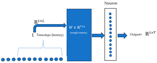
Figure 1.
Linear network predicting future time steps based on past time steps [15].
The output of LTSF-Linear is described as , where is a temporal linear layer and is the input for the variable. This model applies uniform weights across various variables without considering spatial correlations between the variates. Besides LTSF-Linear, a few variations termed NLinear and DLinear were also introduced in [15]. NLinear processes the input sequence through a linear layer with normalization by subtracting and re-adding the last sequence value before predicting. DLinear decomposes raw data into trend and seasonal components using a moving average kernel, processes each with a linear layer, and sums the outputs for the final prediction [15]. This concept has been borrowed from the AutoFormer and FedFormer models [11,12].
Although some research indicates the success of the transformer-based models for time series forecasting, e.g., [10,11,12,16], the LTSF-Linear work in [15] questions the use of transformers due to the fact that the permutation-invariant self-attention mechanism may result in temporal information loss. The work in [15] also presented better forecasting results than the previous transformer-based approaches. However, important research later presented in [14] proposed a transformer-based architecture called PatchTST, showing better results than [15] in some cases. PatchTST segments the time series into subseries-level patches and maintains channel independence between variates. Each channel contains a single univariate time series that shares the same embedding and transformer weights across all the series. Figure 2 depicts the architecture of PatchTST.
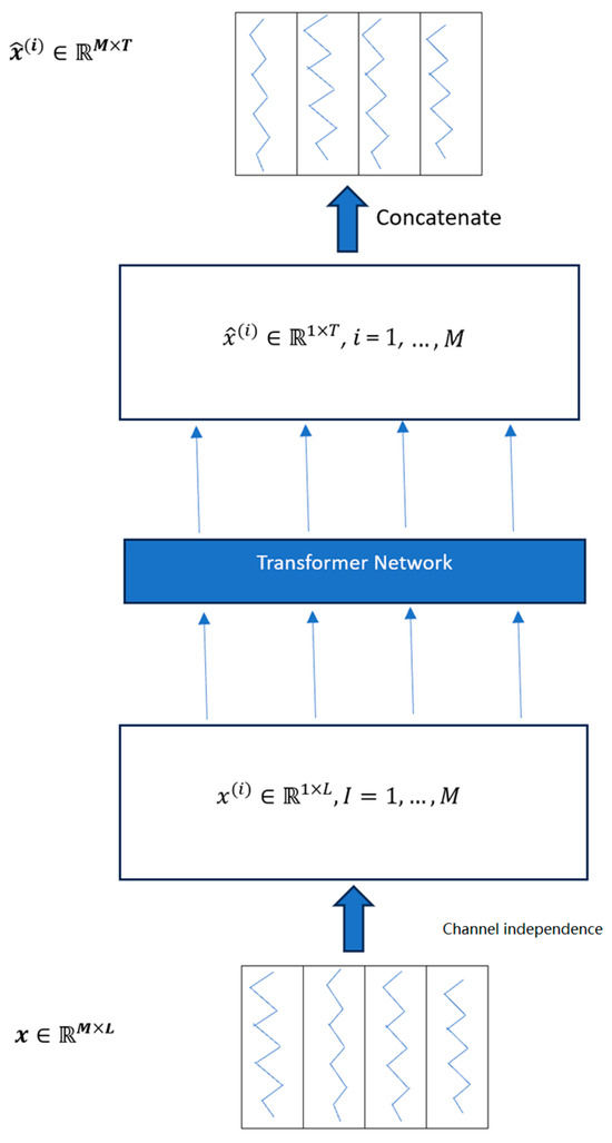
Figure 2.
Architecture of PatchTST [15].
In PatchTST, the ith series for L time steps is treated as a univariate . Each of these is fed independently to the transformer backbone after converting to patches, which provides prediction results for T future steps. For a patch length P and stride S, the patching process generates a sequence of N patches , where . With the use of patches, the number of input tokens can reduce to approximately .
Recently, state-space models (SSMs) have received considerable attention in the NLP and Computer Vision domain [18,19]. For time series forecasting, it has been reported that SSM representations cannot express autoregressive processes effectively. An important recent work using SSM is presented in [20] (termed SpaceTimeSSM) that enhances the traditional SSM model by employing a companion matrix, which enables SpaceTime’s SSM layers to learn desirable autoregressive processes. The time series forecasting represents the input series for p past samples as the following:
Then the state-space formulation is given as follows:
The SpaceTimeSSM composes the companion matrix A as a dxd square matrix:
where =.
We provide a comparison of different time series benchmarks on the SpaceTimeSSM approach in the results Section 4.
3. Methodology
3.1. Proposed Models for Time Series Forecasting
As explained in the previous related works section, there are three competing approaches for time series forecasting: one based on simple linear networks, the second based on transformers where the input series is converted to patches, and channel independence is claimed to be a better scheme, and the third approach based on state-space models with additional enhancements to incorporate autoregressive behavior. We investigated these approaches further to see if better models for time series can be created in at least the first two categories. In the next subsections, we elaborate our enhancements on existing linear- and transformer-based approaches.
3.2. Enhanced Linear Models for Time Series Forecasting (ELM)
We enhanced the LTSF-Linear approach presented in [15] by performing batch normalization and reversible instance normalization. We further combined the information in a novel way using a dual pipeline design as shown in Figure 2. The recent important works, e.g., LTSF-Linear [15], which is based on simple linear networks, and the PatchTST work in [14], based on transformers’ emphasized channel independence, produce better results. We maintain this attribute but further augment the linear architecture with batch normalization. This stabilizes the distribution of input data by normalizing the activations in each layer. It also allows for higher learning rates and reduces the need for strict initialization and some forms of regularization such as dropout. By addressing the internal covariate shift, batch normalization improves network stability and performance across various tasks.
While one of the enhancements in [15], termed NLinear, accommodated for distribution shift in the dataset—by subtracting the last value of the sequence and then adding it back after the linear layer—before doing the final prediction, we incorporate a similar idea in our architecture as a separate stream, as shown in Figure 3.
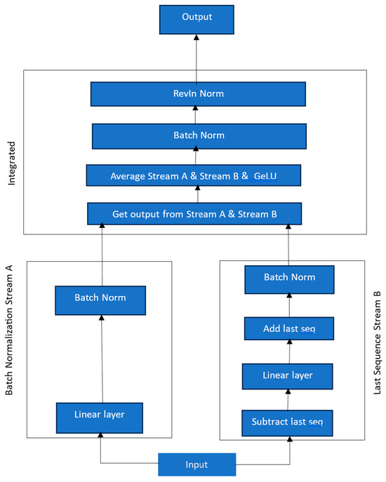
Figure 3.
Our Enhanced Linear Model (ELM).
One difference in our implementation for the distribution shift is that we further add batch normalization to combine temporal information more effectively. From Figure 3, it can be seen that there are two distinct pipelines operating on the input sequence in the beginning. These two streams are then merged together with the values being averaged, and after passing through a non-linearity (GeLU) and another batch normalization layer, we pass through a final Reversible Instance Normalization layer (RevIn). The RevIn originally proposed in [21] operates on each channel of each variate independently. It applies a learnable transformation to normalize the data during training, such that it can be reversed to its original scale during prediction.
We also use a custom loss function that combines the L2 (MSE) and L1 (MAE) losses together in a weighted manner as described below.
where α is a weighting factor between 0 and 1. MSE (input, target) calculates the mean squared error between the input and target values. L1 (input, target) calculates the mean absolute difference between the input and target values. As demonstrated in our results section, our enhanced linear network-based architecture produces better results than existing approaches in many cases on different benchmarks.
To investigate if a different transformer-based architecture may be more suitable for time series forecasting, we adapt the popular Swin transformer [22], which has demonstrated superior results in computer vision. Since the Swin transformer applies attention to local regions, it may have the capability to extract better temporal information. Further, by using shifting windows, it ensures that more tokens are involved in the attention process. We elaborate on this in the next sub-section.
3.3. Adaptation of Vision Transformers to Time Series Forecasting
While one of the recent works on time series forecasting used simple transformer-based architecture (PatchTST [14]) with channel independence, we explore a more intricate transformer architecture, i.e., the Swin transformer [22]. The Swin transformer presents an innovative and streamlined structure for vision-related tasks through the utilization of shifted windows to compute representations. This method tackles the scalability issues inherent to transformers in vision applications by ensuring a linear computational complexity that correlates with the size of the image. It has the additional advantage of overcoming the information loss in the patching process by the use of hierarchical overlapping windows. As a result, it has demonstrated superior results across various computer vision applications. Due to these inherent advantages of the Swin architecture, we adapt it to the time series forecasting domain. We treat the multivariate input series with past steps and d channels as an image and convert it to an appropriate number of patches that are then fed to the Swin model. Due to the use of overlapping, shifted, and hierarchical windows, it has the potential for learning better cross-channel information in predicting future time series data. The architecture of our Swin-based time series model is shown in Figure 4.
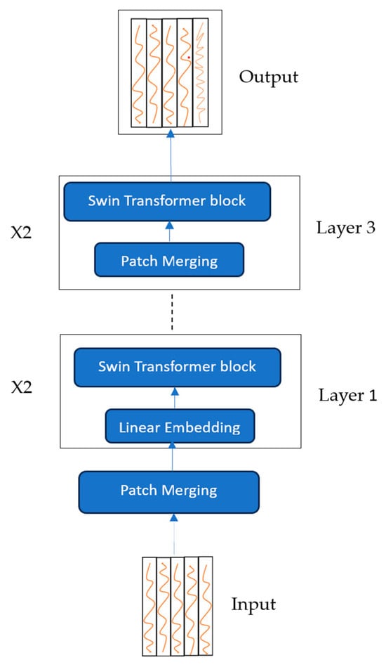
Figure 4.
Adaptation of Swin transformer architecture for time series forecasting.
For feeding the multivariate time series with time steps and d variates to the Swin transformer, the input data need to be converted to patches where is a power of 2. We accomplish this by creating number of patches where and are integers, which are selected to convert the input data to patches. For example, if the input series data have 512 time steps with 7 channels, then and . This results in 256 patches, i.e., . We present the evaluation results on different benchmarks in the next section.
4. Results
We tested our architectures and performed analyses on nine widely used datasets from real-world applications. These datasets consist of the Electricity Transformer Temperature (ETT) series, which include ETTh1 and ETTh2 (hourly intervals), and ETTm1 and ETTm2 (5-minute intervals), along with datasets pertaining to Traffic (hourly), Electricity (hourly), Weather (10-minute intervals), Influenza-like illness (ILI) (weekly), and Exchange rate (daily). The characteristics of the different datasets used are summarized in Table 1.

Table 1.
Characteristics of the different datasets used.
The architecture type of models that we compare to our approach are listed in Table 2.
Table 2.
Architecture types of different models used for comparison.
Table 3 shows the detailed results for our Enhanced Linear Model (ELM) on different datasets and compares it with other recent popular models.
Table 3.
Comparison of our ELM model with other models on the time series datasets.
As can be seen from Table 3, our ELM model surpasses most established baseline methods in the majority of the test cases (indicated by bold values). The underlined values in Table 3 indicate the second-best results for a given category. Our model is either the best or the second-best in most categories. Note that each model in Table 3 follows a consistent experimental setup, with prediction lengths T of {96, 192, 336, 720} for all datasets except for the ILI dataset. For the ILI dataset, we use prediction lengths of {24, 36, 48, 60}. For our ELM model, the look-back window L is 512 for all datasets except Exchange and Illness, which use L = 96. For the other models that we compare to, we select their best prediction based on look-back window size from either of the (96, 192, 336, 720) [14,15]. Metrics used for evaluation are MSE (Mean Squared Error) and MAE (Mean Absolute Error).
Table 4 provides the quantitative improvement over two recent best-performing time series prediction models of PatchTST [14] and DLinear [15]. The values presented are the average of the percent improvement for the four lookback window sizes of 96, 192, 336, and 720. With respect to PatchTST, our model lags in performance on the traffic and illness datasets using the MSE metric but is competitive or exceeds the MSE or MAE metrics on the other benchmarks. The percentage improvement with respect to DLinear is more significant than the PatchTST Model, and our ELM model exceeds the DLinear in almost all dataset categories.
Table 4.
Quantitative improvements of our ELM model with respect to best-performing existing models.
Figure 5 and Figure 6 show the graphs of predicted vs. actual data for two of the datasets with different prediction lengths using a context length of 512 for our ELM model for the first channel (pressure for the weather dataset, and HUFL—high useful load for the ETTm1 dataset). As can be seen, if the data are more cyclical in nature (e.g., HUFL in ETTm1), our model is able to learn the patterns nicely, as shown in Figure 6. For complex data such as the pressure feature in weather, the prediction is less accurate, as indicated in Figure 5.
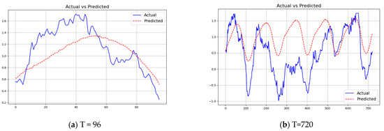
Figure 5.
Predicted vs. actual forecasting using ELM model with L= 512 and T = {96, 720} for Weather dataset.
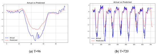
Figure 6.
Predicted vs. actual forecasting using ELM Model with L = 512 and T = {96, 720} for ETTm1 dataset.
Table 5 presents our results on the Swin transformer-based implementation for time series. As explained earlier, we divide the input multivariate time series data into 16 × 16, i.e., 256 patches, before feeding it to a Swin model with three transformer layers. The embeddings used in the three layers are [128,128,256]. As can be seen, the Swin transformer-based approach has the inherent capability to combine information between different channels as well as between different time-steps but does not perform as well as our linear model (ELM); only on the traffic dataset it produces the best result. This could be attributed to the fact that this dataset has the most number of features, which Swin can effectively use for more cross-channel information. Comparing our Swin transformer-based model to the PatchTST model [14] (also transformer-based), the PatchTST that uses channel independence performs better than our Swin-based model. Note that the PatchTST performs worse than our ELM model, which is based on a linear network.
Table 5.
Comparison of our Swin transformer model with other models on the time series datasets. Results highlighted in bold signify the best performance, while those underlined indicate the second-highest achievement.
We also compare our ELM model to the newly proposed state-space model-based time series prediction [20]. State-space models such as Mamba [18], VMamba [19], Vision Mamba [23], and Time Machine Mamba [24] are drawing significant attention for modeling temporal data such as time series, and therefore we compare our ELM model with the recently published work of [20] and [24,25], which are based on state-space models. Table 6 shows the results of our ELM model with the work in [20,24]. In one case, the SpaceTime model is better but most of the time our ELM model performs better than both the state-space and the previous DLinear models. The context length in Table 6 is 720, and the prediction is also 720 time steps.
Table 6.
Comparison of our ELM model to other recently published models. Results highlighted in bold signify the best performance, while those underlined indicate the second-highest achievement.
5. Discussion
One of the recent unanswered questions in time series forecasting has been as to which architecture is best suited for this task. Some earlier research papers have indicated better results with transformer-based models than previous approaches, e.g., Informer [10], Autoformer [11], Fedformer [12], and Pyraformer [16]. Of these models, FedFormer demonstrated much better results as it uses Fourier-enhanced blocks and Wavelet-enhanced blocks in the transformer structure that can learn important patterns in series through frequency domain mapping. A simpler transformer-based architecture yielding even better results was proposed in [14]. This architecture, termed PatchTST, uses independent channels where an input channel is divided into patches. All channels share the same embedding and transformer weights. Since PatchTST is a simple transformer design with a simple independent channel architecture, we explored replacing this design with a Swin transformer with patching across channels. The Swin transformer has the capability to combine information across patches due to its hierarchical overlapping window design. Our detailed experimental results on the Swin architecture-based design did not produce better results as compared to the channel-independent design of PatchTST; however, compared with other transformer-based designs, it yielded improved results in many cases.
To answer the question of the best architecture for time series forecasting, we improve the recently proposed simple linear network-based model in [15] by creating dual pipelines with batch and reversible instance normalizations. We maintain channel independence and our results on the benchmarks show the best results obtained so far as compared to existing approaches in the majority of the standard datasets used in time series forecasting.
6. Conclusions
We perform a detailed investigation as to the best architecture for time series forecasting. We have implemented time series forecasting on the Swin transformer to see if aggregated channel information is useful. We also analyzed and improved an existing simpler model based on linear networks. Our study highlights the significant potential of simpler models, challenging the prevailing emphasis on complex transformer-based architectures. The ELM model developed in this work, with its straightforward design, has demonstrated superior performance across various datasets, underscoring the importance of re-evaluating the effectiveness of simpler models in time series analysis. Compared to the recent transformer-based PatchTST model, our ELM model achieves a percentage improvement of approximately 1–5% on most benchmarks. With respect to the recent linear network-based models, the percentage improvement by our model is more significant, ranging between 1 and 25% for different datasets. It is only when the number of variates in the dataset is large that the Swin transformer-based design we adapt for the time series prediction seems to be effective.
Future work involves the development of hybrid models that leverage both linear and transformer elements such that each contributes to the effective learning of the time series behavior. For example, the frequency domain component as used in FedFormer could aid a linear model when past periodicity pattern is more complex. The recent developments in state-space models and their applications to time series forecasting such as TimeMachine [24,25] (based on Mamba) also deserve further research in optimizing these models for better prediction.
Author Contributions
Conceptualization, M.A. and A.M.; methodology, M.A.; software, M.A.; validation, M.A. and A.M.; formal analysis, M.A.; investigation, M.A.; resources, M.A.; data curation, M.A.; writing—original draft preparation, M.A. and A.M.; writing—review and editing, M.A. and A.M.; visualization, M.A.; supervision, A.M.; project administration, A.M. All authors have read and agreed to the published version of the manuscript.
Funding
The authors received no financial support for this research.
Data Availability Statement
All materials related to our study, including the trained models, detailed results reports, source code, and datasets, are publicly accessible via our dedicated GitHub repository: https://github.com/muslehal/Enhanced-Linear-Model-ELM-, Dataset link: https://drive.google.com/drive/folders/1ZOYpTUa82_jCcxIdTmyr0LXQfvaM9vIy (accessed on 1 April 2024).
Conflicts of Interest
The authors declare no conflict of interest.
References
- Box, G.E.; Jenkins, G.M.; Reinsel, G.C.; Ljung, G.M. Time Series Analysis: Forecasting and Control; John Wiley & Sons: Hoboken, NJ, USA, 2015. [Google Scholar]
- De Livera, A.M.; Hyndman, R.J.; Snyder, R.D. Forecasting time series with complex seasonal patterns using exponential smoothing. J. Am. Stat. Assoc. 2011, 106, 1513–1527. [Google Scholar] [CrossRef]
- Cerqueira, V.; Torgo, L.; Soares, C. Machine Learning vs. Statistical Methods for Time Series Forecasting: Size Matters. arXiv 2019, arXiv:1909.13316v1. [Google Scholar]
- Lim, B.; Zohren, S. Time-series forecasting with deep learning: A survey. Philos. Trans. R. Soc. A 2021, 379, 20200209. [Google Scholar] [CrossRef] [PubMed]
- Salinas, D.; Flunkert, V.; Gasthaus, J.; Januschowski, T. DeepAR: Probabilistic forecasting with autoregressive recurrent networks. Int. J. Forecast. 2020, 36, 1181–1191. [Google Scholar] [CrossRef]
- Hewamalage, H.; Bergmeir, C.; Bandara, K. Recurrent Neural Networks for Time Series Forecasting: Current Status and Future Directions. Int. J. Forecast. 2021, 37, 388–427. [Google Scholar] [CrossRef]
- Sen, R.; Yu, H.F.; Dhillon, I.S. Think globally, act locally: A deep neural network approach to high-dimensional time series forecasting. In Advances in Neural Information Processing Systems 32 (NeurIPS 2019); Neural Information Processing Systems Foundation, Inc. (NeurIPS): San Diego, CA, USA, 2019. [Google Scholar]
- Lai, G.; Chang, W.-C.; Yang, Y.; Liu, H. Modeling Long- and Short-Term Temporal Patterns with Deep Neural Networks. In Proceedings of the SIGIR ‘18: The 41st International ACM SIGIR Conference on Research & Development in Information Retrieval, Ann Arbor, MI, USA, 8–12 July 2018. [Google Scholar]
- Vaswani, A.; Shazeer, N.; Parmar, N.; Uszkoreit, J.; Jones, L.; Gomez, A.N.; Kaiser, Ł.; Polosukhin, I. Attention is all you need. In Advances in Neural Information Processing Systems 30 (NIPS 2017); Neural Information Processing Systems Foundation, Inc. (NeurIPS): San Diego, CA, USA, 2017. [Google Scholar]
- Zhou, H.; Zhang, S.; Peng, J.; Zhang, S.; Li, J.; Xiong, H.; Zhang, W. Informer: Beyond efficient transformer for long sequence time-series forecasting. Proc. AAAI Conf. Artif. Intell. 2021, 35, 11106–11115. [Google Scholar] [CrossRef]
- Wu, H.; Xu, J.; Wang, J.; Long, M. Autoformer: Decomposition transformers with auto-correlation for long-term series forecasting. In Advances in Neural Information Processing Systems 34 (NeurIPS 2021); Neural Information Processing Systems Foundation, Inc. (NeurIPS): San Diego, CA, USA, 2021; pp. 22419–22430. [Google Scholar]
- Zhou, T.; Ma, Z.; Wen, Q.; Wang, X.; Sun, L.; Jin, R. Fedformer: Frequency enhanced decomposed transformer for long-term series forecasting. In Proceedings of the 39th International Conference on Machine Learning PMLR 2022, Baltimore, MD, USA, 17–23 July 2022; pp. 27268–27286. [Google Scholar]
- Li, S.; Jin, X.; Xuan, Y.; Zhou, X.; Chen, W.; Wang, Y.X.; Yan, X. Enhancing the locality and breaking the memory bottleneck of transformer on time series forecasting. In Advances in Neural Information Processing Systems 32 (NeurIPS 2019); Neural Information Processing Systems Foundation, Inc. (NeurIPS): San Diego, CA, USA, 2019. [Google Scholar]
- Nie, Y.; Nguyen, N.H.; Sinthong, P.; Kalagnanam, J. A Time Series is worth 64 words: Long-term forecasting with Transformers. arXiv 2022, arXiv:2211.14730. [Google Scholar]
- Zeng, A.; Chen, M.; Zhang, L.; Xu, Q. Are Transformers effective for Time Series Forecasting? Proc. AAAI Conf. Artif. Intell. 2023, 37, 11121–11128. [Google Scholar] [CrossRef]
- Liu, S.; Yu, H.; Liao, C.; Li, J.; Lin, W.; Liu, A.X.; Dustdar, S. Pyraformer: Low-complexity pyramidal attention for long-range time series modeling and forecasting. In Proceedings of the International Conference on Learning Representations 2022, Online, 25–29 April 2022. [Google Scholar]
- Guillaume, C. Direct multi-step estimation and forecasting. J. Econ. Surv. 2007, 21, 746–785. [Google Scholar]
- Albert, G.; Dao, T. Mamba: Linear-time sequence modeling with selective state spaces. arXiv 2023, arXiv:2312.00752. [Google Scholar]
- Liu, Y.; Tian, Y.; Zhao, Y.; Yu, H.; Xie, L.; Wang, Y.; Ye, Q.; Liu, Y. Vmamba: Visual state space model. arXiv 2024, arXiv:2401.10166. [Google Scholar]
- Zhang, M.; Saab, K.K.; Poli, M.; Dao, T.; Goel, K.; Ré, C. Effectively Modeling Time Series with Simple Discrete State Spaces. arXiv 2023, arXiv:2303.09489v1. [Google Scholar]
- Kim, T.; Kim, J.; Tae, Y.; Park, C.; Choi, J.H.; Choo, J. Reversible instance normalization for accurate time-series forecasting against distribution shift. In Proceedings of the International Conference on Learning Representations 2021, Online, 3–7 May 2021. [Google Scholar]
- Liu, Z.; Lin, Y.; Cao, Y.; Hu, H.; Wei, Y.; Zhang, Z.; Lin, S.; Guo, B. Swin transformer: Hierarchical vision transformer using shifted windows. In Proceedings of the 2021 IEEE/CVF International Conference on Computer Vision, Montreal, BC, Canada, 10–17 October 2021; pp. 10012–10022. [Google Scholar]
- Zhu, L.; Liao, B.; Zhang, Q.; Wang, X.; Liu, W.; Wang, X. Vision mamba: Efficient visual representation learning with bidirectional state space model. arXiv 2024, arXiv:2401.09417. [Google Scholar]
- Wang, Z.; Kong, F.; Feng, S.; Wang, M.; Zhao, H.; Wang, D.; Zhang, Y. Is Mamba Effective for Time Series Forecasting? arXiv 2024, arXiv:2403.11144. [Google Scholar]
- Ahamed, M.A.; Cheng, Q. TimeMachine: A Time Series is Worth 4 Mambas for Long-term Forecasting. arXiv 2024, arXiv:2403.09898. [Google Scholar]
Disclaimer/Publisher’s Note: The statements, opinions and data contained in all publications are solely those of the individual author(s) and contributor(s) and not of MDPI and/or the editor(s). MDPI and/or the editor(s) disclaim responsibility for any injury to people or property resulting from any ideas, methods, instructions or products referred to in the content. |
© 2024 by the authors. Licensee MDPI, Basel, Switzerland. This article is an open access article distributed under the terms and conditions of the Creative Commons Attribution (CC BY) license (https://creativecommons.org/licenses/by/4.0/).