Abstract
The theoretical basis for the Eddy Damped Markovian Anisotropic Closure (EDMAC) is formulated for two-dimensional anisotropic turbulence interacting with Rossby waves in the presence of advection by a large-scale mean flow. The EDMAC is as computationally efficient as the Eddy Damped Quasi Normal Markovian (EDQNM) closure, but, in contrast, is realizable in the presence of transient waves. The EDMAC is arrived at through systematic simplification of a generalization of the non-Markovian Direct Interaction Approximation (DIA) closure that has its origin in renormalized perturbation theory. Markovian Anisotropic Closures (MACs) are obtained from the DIA by using three variants of the Fluctuation Dissipation Theorem (FDT) with the information in the time history integrals instead carried by Markovian differential equations for two relaxation functions. One of the MACs is simplified to the EDMAC with analytical relaxation functions and high numerical efficiency, like the EDQNM. Sufficient conditions for the EDMAC to be realizable in the presence of Rossby waves are determined. Examples of the numerical integration of the EDMAC compared with the EDQNM are presented for two-dimensional isotropic and anisotropic turbulence, at moderate Reynolds numbers, possibly interacting with Rossby waves and large-scale mean flow. The generalization of the EDMAC for the statistical dynamics of other physical systems to higher dimension and higher order nonlinearity is considered.
1. Introduction
Orszag [1] proposed the Eddy Damped Quasi Normal Markovian (EDQNM) model as an efficient and realizable closure for three-dimensional (3D) isotropic turbulence. The first numerical study of the EDQNM was made by Leith [2], who formulated and solved it for two-dimensional (2D) isotropic turbulence. Herring [3] derived a statistical dynamical closure for 2D anisotropic turbulence that generalized the EDQNM to situations without transient waves. The EDQNM is computationally efficient because it is Markovian and consists of just the equations for the single-time two-point cumulant in spectral space with an analytical expression for the triad relaxation function. However, as we discuss and analyze in detail in this article, the EDQNM is not guaranteed to be realizable for anisotropic turbulence interacting with transient waves. In contrast, the Eddy Damped Markovian Anisotropic Closure (EDMAC), for which we formulate the theoretical basis, is realizable.
One can arrive at the EDQNM in various ways, as discussed, for example, by Lesieur [4], with our preference being from a reduction of the more fundamentally based Eulerian Direct Interaction Approximation (DIA) of Kraichnan [5]. The DIA is a more complex non-Markovian closure that is founded on renormalized perturbation theory (reviews of closures are presented in Refs. [4,6,7,8,9,10,11,12,13]). These reviews present analyses of the relative performance of the various closure models. The form of the eddy damping in the EDQNM is chosen to be consistent with the forward energy cascading inertial range of 3D isotropic turbulence and the forward enstrophy cascading inertial range of 2D turbulence.
Starting from the DIA, the EDQNM may be obtained by using a Markovian form for the response function and using the current-time FDT (Fluctuation Dissipation Theorem)
for and for . In Equation (1), is the response function, is the two-time spectral cumulant, and the current-time single-time cumulant at wavenumber (or strictly wavevector) . In the EDQNM, the response function is also specified by an analytical form consistent with either the 2D or 3D inertial ranges. With these modifications, the time-history integrals of the DIA can be performed analytically to determine a triad relaxation function that enters the cumulant equation (see Section 7). In the EDQNM, the strength of eddy damping is specified by an empirical constant, as distinct from the DIA, which has no empirical parameters.
The EDQNM closure has the advantage of being very computationally efficient since it scales like , where is the length of the time integration. This contrasts with the DIA non-Markovian closure that scales as , because the two-point cumulants and response functions satisfy integro-differential equations. Although, we should note that the efficiency of the DIA can be improved to scaling like . This can be performed by using the three-point cumulant in periodic restarts of the DIA closure numerical model [14,15,16,17].
The DIA is closely related to the Self Consistent Field Theory closure (SCFT) of Herring [18,19] and the Local Energy-Transfer Theory closure (LET) of McComb [6,20,21]. The SCFT and LET closures are also non-Markovian and, despite being originally derived by different methods, can in fact also be obtained by modifications of the DIA equations. These three Eulerian non-Markovian closures all have the same single-time two-point closure equation. However, the SCFT and LET use the prior-time FDT [12] (Equation (1)) defined by
for where is the prior-time single-time cumulant. In the SCFT, the response function, identical to that for the DIA, is taken as fundamental and the two-time cumulant is obtained from the prior-time FDT. For the LET the two-time cumulant, identical to that for the DIA, is fundamental, and the response function is derived from the FDT in Equation (2). In this study, we focus on the derivation of Markovian closures from the DIA closure, but we could equally consider the SCFT or LET as the starting points.
The EDQNM closure has been widely used in many studies and applications, as reviewed in Refs. [4,9,10,11,12,22]. As emphasized in the detailed study of Bowman et al. [23], the EDQNM may not be realizable in the presence of transient waves such as drift waves in plasmas or, equivalently, Rossby waves in geophysical flows. In some studies, the waves have been assumed to be slowly varying, and the quasi-steady state form of the triad relaxation function is used to avoid possible singular behavior [22,23,24,25,26,27,28,29]. In other studies, modified forms of quasi-normal Markovian closures have instead been used [30,31].
The reason that the EDQNM may not necessarily be realizable with transient waves is because the oscillations of the propagating waves mean that the real part of the triad relaxation functions in the EDQNM may, on occasions, become negative. Bowman et al. [23] found that the same problem also occurs if the prior time FDT in Equation (2) is used. However, they showed that a realizable Markovian closure could be obtained by using a FDT that is essentially a half-way house between the current-time and prior-time FDTs. This FDT, which we call the correlation FDT, is given by
for . Bowman et al. [23] called their closure the Realizable Markovian Closure (RMC). Unlike the EDQNM closure, for which the triad relaxation functions have analytical expressions, the RMC relaxation functions need to be evaluated by solving a system of auxiliary differential equations. Hence the RMC is less computationally efficient than the EDQNM. Hu et al. [32] used the RMC in studies of the Hasegawa–Wakatani two-field equation of plasma physics. Bowman and Krommes [33] further developed and applied realizable Markovian closures for homogeneous turbulence in the presence of waves. They considered the interaction of drift waves (essentially Rossby waves) and anisotropic turbulence with the single-level Charney–Hasegawa–Mima model. They also formulated a realizable test-field model (RTFM), a generalization of Kraichnan’s [34] test-field model (TFM), for turbulence in the presence of transient waves.
Traditionally, closure theory, including Markovian closures, like the EDQNM [1,2], have focused on the forward energy cascade of 3D turbulence and the forward enstrophy cascade of 2D turbulence in decaying and steady state systems. The EDQNM damping is normally specified to be consistent with these forward inertial ranges. Two-dimensional turbulence also has an inverse energy cascade, with a steady state inertial range of [35]. With differential rotation on a –plane, supporting Rossby waves, the turbulence becomes anisotropic, with preferential zonal motion. This was noted by Rhines [36] based on theory and direct numerical simulations (DNS) and by Holloway and Hendershott [37] in studies with a modified TFM. Their TFM did not cater for transient Rossby waves, but required an approximate steady state triad relaxation function to guarantee realizability [33]. Rhines [36] proposed that, under suitable conditions, the fluid velocities follow an inverse power law in steady state where is the wavenumber, the magnitude of the total wavevector. Chekhlov et al. [38] performed a set of DNS experiments of 2D turbulence on a –plane forced by small scale forcing. They found support for the scaling of Rhines, for the zonal components with which followed a power law. However, the rest of the spectrum followed the inverse energy cascade, emphasizing the anisotropy induced by the Rossby waves [22,24,25,26,27,28,29,37]. This is further discussed in the review by Galperin et al. [39]. Krommes and Parker [40] also discuss the application of homogeneous closures to circulations with zonal flow generation through inverse cascades, such as on the giant planets and their moons, and to plasma physics (see also the reviews in Refs. [41,42]). They note, however, that real flows are generally inhomogeneous and “statistically inhomogeneous solutions with nontrivial mean fields can emerge from a statistically homogeneous state by spontaneous symmetry breaking”. Indeed, Frederiksen [43] shows that just an infinitesimal topographic perturbation can cause such symmetry breaking with the mountain torque driving a mean westward zonal flow on the –plane and solid body rotation on the sphere. This symmetry breaking may considerably modify the structures of the larger scale flows in the inverse cascades.
For the earth’s atmosphere, with a Rossby radius of deformation around 1000 km, the larger scales of turbulent 2D and quasigeostrophic flows are determined by heating, topography, and baroclinic instability that override the inverse cascades [4]. It is 2D homogeneous flows, in typical atmospheric parameter ranges, with forward enstrophy cascades, and the analogous 3D homogeneous flows with forward energy cascades, that are of primary interest in our current study. For flows in these parameter ranges, the large-scale flows can be specified to have realistic initial spectra or driven towards such states with the smaller scales evolving towards their statistically steady states. In this way, studies with homogeneous closures can throw considerable light onto the essential issues of the more complicated inhomogeneous turbulence interactions.
In the last few years, Markovian closures have also been developed for inhomogeneous turbulence interacting with mean flows, Rossby waves, and topography by Frederiksen and O’Kane [12,44,45]. Three types of Markovian Inhomogeneous Closures (MICs) were developed [44], as well as three types of abridged MICs [45]. For the abridged MICs, the mean field trajectory in the time history integrals is replaced by the current-time mean field and results in slightly more efficient closures. To date, all the MIC variants have been developed as modifications of the inhomogeneous non-Markovian QDIA closure [46,47,48].
The QDIA was developed for 2D inhomogeneous turbulent flows interacting with mean fields and topography by Frederiksen [46]. It was extended to include Rossby waves (Frederiksen and O’Kane [47]) and to multi-level and multi-field models for classical and quantum field theories (Frederiksen [48,49]). It was numerically implemented by O’Kane and Frederiksen [17] and subsequently used in further studies of turbulence dynamics, interactions with topography and Rossby waves, predictability of transitions between strong zonal flows and blocking, in data assimilation and for determining subgrid-scale parameterizations. The literature is reviewed in Refs. [45,49].
The MICs are obtained from the QDIA closure by assuming one of the three FDTs. They can be combined as:
for and for . The current-time FDT is recovered when , the prior-time FDT has and the correlation FDT has .
In the numerical studies of Frederiksen and O’Kane [44,45], it was found that both the MICs [44] and abridged MICs [45] closely reproduced the statistics of large ensembles of DNS in simulations of inhomogeneous turbulence interacting with mean flows, Rossby waves and topography at low Reynolds numbers. While the MIC and abridged MIC models are more computationally efficient than the non-Markovian QDIA closure, the relaxation functions still need to be calculated by solving auxiliary differential equations, as for the RMC of Bowman et al. [23]. A still more efficient inhomogeneous Markovian closure with analytical relaxation functions, the Eddy Damped Markovian Inhomogeneous Closure (EDMIC), was also developed by Frederiksen and O’Kane [45].
In a recent tribute to Jack Herring [12], and review of his major achievements in statistical dynamical fluid dynamics, it was noted that it is possible to generalize the EDQNM to a closure that is realizable in the presence of transient Rossby waves interacting with anisotropic turbulence. The resulting Eddy Damped Markovian Anisotropic Closure (EDMAC) involves a frequency renormalization of the eddy damping and by construction is as efficient as the EDQNM.
The major aims of this article are as follows:
- To provide a theoretical motivation for the realizable EDMAC based on renormalized perturbation theory.
- To generalize the EDMAC model for the interaction of anisotropic turbulence with transient Rossby waves in the presence of transient large-scale flows.
- To establish conditions under which the real part of the triad relaxation functions is positive semi-definite when the large-scale flow and Doppler shifted Rossby wave frequency have general time dependencies.
- To examine the extent to which the frequency-dependent contribution to the eddy damping in the EDMAC model changes the evolved energy and palinstrophy spectra and Reynolds number and skewness, compared with the EDQNM, for rapidly evolving moderate Reynolds number turbulence interacting with Rossby waves.
The methodology we apply for developing the realizable EDMAC model has parallels with the approach used by Frederiksen [46] to formulate the inhomogeneous quasi-diagonal direct interaction approximation (QDIA) closure. Frederiksen [46] developed the QDIA using a renormalized perturbation theory approach in which the isotropic problem was treated as the zero-order problem. The anisotropic and inhomogeneous terms were considered as small and multiplied by a perturbation parameter , prior to renormalization. Here we apply this approach to formulate the EDMAC.
The plan of this article is as follows. In Section 2, we present the equations for two-dimensional barotropic flows on a generalized –plane and with large-scale advection by a mean flow. The dynamical flow equations are then converted to the equivalent form in Fourier space in Section 3. This is necessary for the subsequent formulation, in Section 4, of non-Markovian closures for the interaction of anisotropic turbulence with Rossby waves. These generalized DIA, SCFT, and LET closures have the same single-time cumulant equation and are equally suitable for reducing to the Markovian anisotropic closures (MACs) formulated in Section 5. There, three variants of the MACs are formulated using the three versions of the FDT that are summarized in Equation (4). As well, in Section 5, the prognostic equations for the relaxation functions that close the Markovian statistical dynamical equations are derived. In Section 6, we focus on the Markovian variant for which the current-time FDT in Equation (1) is imposed, and note the simplifications in the structure of the closure that then entail. The EDMAC model is formulated in Section 7 and in Section 8 the sufficient conditions for the realizability of EDMAC in the presence of transient Rossby waves are established. Generalization of the realizable EDMAC to other physical systems with transient waves and to higher dimension and higher order nonlinearity is considered in Section 9. In Section 10, numerical integrations of the EDMAC and EDQNM models are reported on for isotropic and anisotropic 2D turbulence of various complexity. The implications of the results and our conclusions are presented in Section 11. The derivation, based on renormalized perturbation theory, of the generalized DIA closure from which our analysis starts is located in Appendix A. The Langevin equation for the EDMAC model that guarantees realizability is presented in Appendix B.
2. Two-Dimensional Barotropic Flows on a –Plane with Large-Scale Advection
We formulate our statistical dynamical equations for the case of two-dimensional or barotropic flows, although the generalization to three-dimensional flows can also be accomplished, as described in Section 9. Turbulent flows in planar geometry are considered on a generalized –plane, and include a large-scale advection by a wind . The total flow is described by the streamfunction where represents the small scales. Throughout this paper, we present theoretical and numerical results for flows on the doubly periodic plane with .
2.1. Large-Scale Flow Equation
The large-scale flow is kept the same in each realization of the smaller scales, and effectively just modifies the beta effect. We include possible relaxation to a mean large-scale flow with strength so that may evolve with time according to
In the absence of the relaxation forcing and dissipative drag, is separately conserved.
2.2. Barotropic Vorticity Equation for the Small Scales
The evolution of the small scales is described by the barotropic vorticity equation on a –plane with the advective wind modifying the Rossby wave propagation:
The Jacobian is defined by:
and the relationship between the vorticity and the stream function is
where is the Laplacian.
The results that we present can also easily be extended to turbulent flow on a sphere, where is the analogue of the solid body rotation. Indeed, the structure of Equation (6) is the same as for flow on a sphere. The wavenumber is the analogue of that on the sphere with corresponding to the vorticity of the solid body rotation. In Equation (6), is the viscosity, is the beta effect and specifies possible external forcing.
3. Dynamical Equations in Fourier Space
The statistical dynamics of turbulent flows is most conveniently analyzed in spectral space. For the doubly periodic domain, the equations are transformed into Fourier space by spectral representations of the fields in the form:
where the spectral coefficients
The wavenumbers in the and directions are and with the wavenumber vector and the magnitude . The spectral coefficients satisfy the complex conjugate symmetry which guarantees that the fields in physical space are real. The domain in Equation (9) can be general, but we suppose that it contains the integer wavenumbers in a circular area (to be specified) that excludes the origin . The vorticity equation in spectral space then takes the form:
Here, we have generalized the form of the viscosity which corresponds to more general dissipation operators than the Laplacian in Equation (6). In Equation (11), the delta function if and 0 if . The interaction coefficient is defined by:
The Doppler shifted Rossby wave frequency is given by the dispersion relationship:
where the Rossby wave frequency is
and
We note that in the case of inviscid flows Rossby waves of the form are exact solutions to Equation (6).
4. Non-Markovian Closures for Turbulence and Rossby Waves
The aim with closure theory is to develop statistical dynamical equations that describe the evolution of the low order moments or cumulants for infinite ensembles of flow fields. To start the process, we first represent a given member by its mean, the one-point cumulant, , and the deviation from the mean, . We consider homogeneous turbulence in this study for which the small scales have zero mean:
Since the mean is zero, the deviation also satisfies Equation (11) (with ). The mean forcing also needs to be zero:
4.1. Generalized DIA Closure for Anisotropic Turbulence and Rossby Waves
To formulate the realizable EDMAC model equations, we start with the DIA closure that is slightly generalized as derived in Appendix A. For homogeneous anisotropic turbulence, the DIA closure describes the evolution of the two-time two-point cumulant
and response function
which is the ensemble average of individual responses. The response function for an individual disturbance is
The response function measures the change in the field due to an infinitesimal perturbation in the forcing at an earlier time. Here, denotes the functional derivative.
The two-time two-point cumulant equation for the generalized DIA, as formulated in Appendix A, is given by
This is the case for , while for we have . Here, the last term in Equation (21) arises from
where is the initial time and the bare noise
Also, the nonlinear damping and nonlinear noise are derived in Appendix A and given by:
and
The expressions for and are also derived in Appendix A, and are given by:
and
In a similar way, the response function equation can be derived as
for , and the Dirac delta function means that .
The final equation needed for the DIA closure is that for the single-time two-point cumulant:
The system of DIA equations is started from the initial conditions and . Equation (29) can also be simplified to the form:
since the and terms cancel because
4.2. The Abridged DIA Closure for Anisotropic Turbulence and Rossby Waves
As a first step towards developing Markovian Anisotropic Closures (MACs) for the interaction of turbulence and Rossby waves, we present, in this subsection, an abridged generalized DIA closure. We consider the situation where the large-scale field is slowly varying in the time history integrals:
Thus, the abridged DIA closure equations are again given by Equations (21) to (25) and (28) to (30), but with Equations (26) and (27) replaced by
and
where the Markov approximation in Equation (32) is denoted by the superscript .
4.3. Generalized SCFT and LET Closures for Ansotropic Turbulence and Rossby Waves
We can also arrive at generalized SCFT and LET closures from the generalized DIA closure in the usual way by invoking the prior-time FDT in Equation (2). For the generalized SCFT this FDT determines the two-time cumulant instead of Equation (21). For the generalized LET closure, the FDT determines the response function instead of Equation (28). For the corresponding abridged SCFT and LET closures, Equations (33) and (34) again replace Equations (26) and (27).
5. Statistical Dynamical Equations for Markovian Anisotropic Closures
General Formulation of Markovian Anisotropic Closures
As the next step towards formulating the realizable EDMAC model with analytical form for the relaxation function we outline the theory of associated Markovian Anisotropic Closures (MACs). The MACs are described by the single-time cumulant equation and auxiliary integral, or equivalent differential, equations for two relaxation functions. The MACS result from employing any of the three FDTs in Equation (4) and Markovianizing the generalized DIA in Section 4. As noted there the version with is the current-time FDT, the correlation FDT, and the prior-time FDT. The corresponding MACs are denoted by . The MACs can be formulated using the general expressions for and in Equations (26) and (27). However, since our final aim is to simplify the MAC with to the realizable EDMAC we make the derivations from the abridged DIA with and given in Equations (33) and (34).
The single-time two-point cumulant equation for the abridged generalized DIA, (and as well for the corresponding SCFT and LET closure) that is also used for each of the MAC models can be written as:
We note that is real. The and terms can be written in the following convenient forms for subsequent Markovianization. Firstly,
where
As well,
with
The bare forcing spectrum
In a similar way,
with
and
Here, the dissipation and Rossby wave dispersion term is
Next, the three versions of the FDT in Equation (4) are applied and this simplifies the nonlinear noise and nonlinear damping terms in Equations (36) and (41). Then, the time history integrals can then be expressed by relaxation functions and for . The integral representations for and can in turn be replaced by differential equations that augment Equation (35) for the single-time cumulant. This system is therefore Markovian with the variant with also guaranteed to be realizable since it is a generalization of the RMC model of Bowman et al. [23].
From Equations (36), (37) and (4) we have
with the triad relaxation function
As well,
where the relaxation function
In a similar way, and simplify to
where
and
with
The equation for the single-time cumulant can also be written in the form:
and for consistency the response function equation becomes:
The renormalized dissipation and noise functions in Equations (53) and (54) are defined by
with the contributing terms given above.
The modified form of the response function can also be written as:
for with and is real. Here we have used the general FDT in Equation (4) and is then also obtained from in Equation (24) and has the expression:
The simplified form of the response function in Equation (54) together with the FDT in Equation (4) means that the relaxation functions in Equation (46) and in Equation (48) can be replaced by differential equations. The differential equation for is:
where and is given in Equation (55). The corresponding differential equation for is:
with .
Now, the closure for any of the three MACs with is Equation (53) for the single-time cumulant , augmented by the differential equations for in Equation (58) and in Equation (59). The replacement of the integral forms for and by the differential equations has made the system Markovian. The auxiliary differential equations for and of course generate the same information as the time history integral forms but for long time simulations are more efficient. Nevertheless, analytical forms for and result in even more efficient closures, such as the EDQNM and EDMAC of Section 7. Each of the three formulated in this section is realizable for pure turbulence without transient wave phenomena. The MAC model with is also realizable when transient Rossby waves are present [23]. We note that, in fact,
so these terms can be dropped from Equation (53).
6. Markovian Anisotropic Closure with Current-Time FDT
In this Section, we consider the further simplifications of the models when so that the current-time FDT is used. This is a step towards the formulation of the EDMAC model, in the following Section, with analytical forms for the relaxation functions. When , Equation (53), for the single-time cumulant, simplifies to:
where, for white noise, . Here, we have used Equation (60) and the fact that the interaction coefficients have the properties that , and . Also note that single-time cumulants are real. As well, to establish Equation (61), we have used the fact that the triad relaxation function is symmetric in the three wavenumber indices:
as seen from Equation (46), when .
Similarly, the expression for simplifies to
The corresponding differential equation forms of and are given in Equations (58) and (59) with the simplification that on the right-hand sides. Also, when , Equation (50) reduces to
where we have used the properties of the interaction coefficients noted above and the symmetry properties of the triad relaxation function. Also, Equation (52) becomes
We also note that if the current-time FDT in Equation (1) is used (with in Equation (4)), then the expression for the response function simplifies to
for with and is defined in Equation (57). Here we note that the expression for in Equation (64) where can also be written as
and is given in Equation (52) with . Thus, Equation (66) is of course just Equation (54) written out in detail when .
For general , corresponding to the three FDTs, the solution to the response function differential Equation (54) (and Equation (66)) is
where is defined in Equation (55). Of course, when , and are given in Equations (64) and (65). We also note that, for the triad relaxation function in Equation (46) reduces to
7. Realizable Eddy-Damped Markovian Anisotropic Closure
In this Section, we consider further simplifications that lead to the realizable EDMAC model. The approach involves the Markovian approximation for the damping terms, as in the EDQNM, and leads to analytical expressions for the relaxation functions.
7.1. Markovian Approximation and Analytical Eddy Damping
Thus, with the Markov approximation for , namely , the response function takes the simple form:
since integral in Equation (68) can then be evaluated. Also, the integrals in the expression for the triad relaxation function in Equation (69) can also be evaluated to give
For the EDMAC model, like the EDQNM closure, we use a parameterized form for the eddy damping , which appears in Equation (71) through , and that is consistent with the forward enstrophy cascading inertial range:
where
Here is a positive dimensionless parameter. This local form for is consistent with that of Leith [2] for 2D turbulence, and Orszag [1] used a corresponding local form for 3D turbulence applicable to the forward energy cascading inertial range. Note, however, that our approach applies equally if an integral form over wavenumbers (Pouquet et al. [50]; Herring et al. [51]) is used instead for the eddy damping.
7.2. Frequency-Dependent Damping from Renormalized Perturbation Theory
Here, we consider the problem where the damping is taken as the zero-order term and the Doppler-shifted frequency is supposed to be a small perturbation of order . Then, we carry out the perturbation expansion as in Appendix A with the result that:
Here, is the zero-order response function, as in Appendix A. We have assumed that and are slowly varying, and then we can evaluate the integral to obtain:
In formulating the EDQNM model, is specified to have the form in Equation (72) (or the integral form of Pouquet et al. [50]) from the initial conditions rather than developing from zero. In the same way, we take the quasi-steady state expression for the contribution from . The result is:
Renormalizing, we obtain our required expression for establishing the realizable EDMAC model:
Thus, comparing the frequency-dependent term , for the MAC model, in Equation (65) with Equation (77), we see that
where the above analysis indicates that . We leave the constant in Equation (78) and in the following analysis, since it could be used as an empirical parameter in situations when the wave frequency is not small compared with the eddy damping. From Equation (52), with , and Equation (78), we see that
where is given in Equation (73).
Combining the above results with those of Section 7.1, we find
where
is the frequency renormalized damping. Thus, the EDMAC response function becomes:
and the EDMAC triad relaxation function:
The EDMAC model is then defined by Equation (61), but with in Equation (83) replacing . In Section 8, to follow, and Appendix B, we determine sufficient conditions for the EDMAC to be realizable. The EDMAC has the same structure as the EDQNM, but with just replacing in the triad relaxation function. It is essentially as computationally efficient as the EDQNM, as discussed further in Section 10, but with the advantage of guaranteed realizability.
8. Conditions for Realizability of EDMAC with Variable Rossby Wave Frequency
In this Section, we determine sufficient conditions on the damping , in Equation (81), so that ; that is, so that the real part of the triad relaxation in Equation (83) is a positive semi-definite. We consider the general case where the Doppler shifted frequencies are time-dependent and are not necessarily monotonic.
The results of Section 7 suggest that is an appropriate value for small . More generally, for larger , the constant may be regarded as an empirical factor that is specified. Our aim is therefore to determine sufficient conditions on for realizability of the EDMAC model.
The triad relaxation function, , in Equation (83) for the EDMAC model, can be written in simplified form as:
where we take (without loss of generality). In Equation (84),
with for triad interactions. The real part of the relaxation function that appears in the EDMAC model for the two-point cumulant (Equations (53) and (61) with superscript replaced by ) is then given by:
Then, sufficient conditions for are determined as follows. In Equation (86), we can replace by for , since both and are even functions of . On the basis of the analysis in Section 7.2, we suppose that
Firstly, we see that , for , since then
Secondly, from Equation (87), we see that for ,
Further, in general,
and thus, for ,
This then means that , for . Sufficient conditions for the validity of Equation (87) is that each wavevector component satisfies
In turn, the inequalities in Equation (92) are valid provided , as seen by solving quadratic equations.
9. Generalizations of the EDMAC Model
The analysis of Section 8, determining sufficient conditions for , can in fact be generalized to all dimensions and with components interacting instead of just the three. The condition for this is again that since none of the argument in Section 8 depends on the dimension or the number of interacting components. It just requires that and , with a general dispersion relationship, is finite.
This again has important implications for general EDQNM-type closures for which realizability is dependent on the relaxation function having positive semi-definite real part. Suppose that the relaxation function is given by the right hand side of Equation (84), but with replacing . Then, including the effects of frequency renormalized damping, , as specified in Equation (85), results in the associated realizable EDMAC model.
It is straightforward to extend the EDMAC model to 2D turbulent flows and Rossby waves on a differentially rotating sphere [9,27]. It is also a simple matter to extend the EDMAC to 3D quasigeostrophic turbulent flows and waves in the model in Appendix B of Frederiksen [48] generalized to rotating flows on a –plane and on a sphere. The EDQNM closure of Carnevale and Frederiksen [25] for two-dimensional internal gravity waves used the quasi-steady state form for the triad relaxation function to ensure realizability. This restriction can be removed, and transient internal gravity waves considered, by going to the EDMAC model form for the relaxation functions. Realizability can be assured by using the frequency renormalized form of the damping in Equation (81) where is replaced by the internal wave frequency with (Equation (2.7c) of Ref. [25]).
One might also expect to be able to develop suitable generalizations of the EDMAC to 3D Navier–Stokes turbulence [1,10,22], including with rotation and waves. In particular, the study by Cambon and Jacqui [52] considered 3D anisotropic turbulence subject to rotation with different Rossby numbers and waves in EDQNM type models. They also used the quasi-steady state form for the triad relaxation function that ensures realizability. This might be extended to the transient regime form by using a frequency renormalized damping as for the EDMAC model. Rose and Sulem [53] and Clark et al. [54] formulate the EDQNM closure for isotropic turbulence in general dimensions, and it would be of interest to see if this could be generalized to anisotropic turbulence, with preferred zonal motion [27,36,37], subject to differential rotation and waves with the realizable EDMAC.
There are, of course, also important physical systems for which the nonlinearity is of a higher order than quadratic. Two examples, with cubic nonlinearity in the field equations, are the nonlinear Schrodinger equation (Nazarenko [55] reviews the literature) and the Klein Gordon equation with Lagrangian (Frederiksen [49] reviews the literature). The nonlinear Schrodinger equation is of major importance in the study of optical turbulence, plasma physics and continuum mechanics [55,56] and the Klein Gordon equation in the classical and quantum statistical dynamics of Bose–Einstein condensation and scalar field theory [49,57,58]. In spectral space, in Equation (85), corresponding to quartic interactions, would then be needed in closures including EDMAC, EDQNM, and resonant interaction or wave turbulence models [25,49,54,55,56,57,58] of such phenomena.
10. Comparison of Closure Integrations for Turbulence and Rossby Wave Dynamics
In this Section, we compare closure calculations with the EDQNM and EDMAC models for isotropic turbulence and anisotropic turbulence with Rossby waves and possibly a large-scale mean flow. The integrations start from the isotropic spectrum B that was studied by Frederiksen and Davies [15,16] for closures with discrete spectra and which is very similar to the continuous spectrum II of Herring et al. [59]. These spectra were used by Herring et al. [59] and Frederiksen and Davies [15] in studies of the comparison of closures with DNS for 2D isotropic turbulence. In particular, the continuous wavenumber formulation of the DIA closure was compared with discrete wavenumber DNS by Herring et al. [59], while Frederiksen and Davies [15] used the discrete formulation for both. In both studies, the DIA closure, and its associated SCFT and LET closures in Ref. [15], were found to underestimate the small-scale amplitudes (Figures 22 and 23 of Ref. [59]; Figures 3 and 4 of Ref. [15]). However, the discrete closures [15] were found to be in better agreement with the statistics of DNS than the continuous closures [59]. O’Kane and Frederiksen [17] also used spectrum B [15,16] for the initial transient spectrum in studies of inhomogeneous turbulence interacting with mean flows and topography with the QDIA closure.
A regularized version of the DIA, the RDIA, in which the wavenumber ranges of interaction are restricted in the response function and two-time cumulant [16], was found to give quite close agreement with the statistics of DNS at the expense of an empirical parameter . This is shown in Figures 1 and 2 of Ref. [16], although there does seem to be a tendency of the smallest scales of the DNS to kick up somewhat in all these studies [15,16,59].
The EDQNM and EDMAC models also depend on the empirical parameter in Equation (72). For the EDMAC model, we have estimated to be the strength of the frequency-dependent damping in Section 7.2, and we use that value. More generally, if the waves do not satisfy the formal requirement of being of small amplitude, then could also be regarded as an empirical parameter. Here, our aim is first to compare the EDQNM and EDMAC models for a commonly used value of [2,9] for 2D turbulence and then to discuss the generality of our findings for a range of .
10.1. Diagnostics
The evolved closure integrations for the EDQNM and EDMAC models are compared in terms of the similarity of their evolved kinetic energy and palinstrophy spectra and Reynolds number and skewness. These diagnostics are defined as follows. Firstly, we specify the energy,
enstrophy,
palinstrophy,
enstrophy dissipation,
and palintrophy production,
Here, is defined in Equation (61). The large-scale Reynolds number and skewness are then specified by
and
The transient kinetic energy spectra, and palinstrophy spectra, averaged over circular bands, are defined by:
and
with the set is defined by
The band-average is over all within a band of unit width at a radius .
10.2. Initial Spectra and Parameter Specifications
In this subsection, we specify the parameters and initial spectra used in our closure calculations. They are based on the related studies in Refs. [9,15,16,47,59]. The length scale used is of one half the earth’s radius, , and time scale is the inverse of the earth’s rotation rate, . The the –effect is zero in the isotropic integrations and (corresponding to in non-dimensional units) in the anisotropic runs. This is characteristic of the earth’s differential rotation at latitude, and the parameter in Equation (6). We use a (bare) viscosity coefficient of (non-dimensional ). In the closure integrations, the mean eastward flow is either zero or has a speed of (non-dimensional ). The closure runs are all unforced, with in Equation (6) and the drag on the large-scale flow in Equation (5). The parameter in Equation (72) that specifies the strength of the eddy damping is specified at as used in [9]. We have, however, checked that the broad conclusions regarding the similarity of the closure calculations described in Section 10.3 to follow hold for a wide range of down to 0.01. The closure calculations are performed at a resolution of circular truncation C64 where . All integrations proceed to (non-dimensional ) with a time step of (non-dimensional ). The time stepping is performed with a predictor-corrector scheme.
The closure calculations start from Gaussian initial conditions with for spectrum B of Frederiksen and Davies [15,16]:
From this spectrum, the closure integrations proceed with one run being for isotropic turbulence, denoted run , and three runs for anisotropic turbulence with Rossby waves, denoted runs to . The particular values of nondimensional , , of Equation (78), and that are used in runs and to are given in Table 1.

Table 1.
Non-dimensional parameters specifying the isotropic and three anisotropic closure runs.
10.3. Moderate Reynolds Number Closure Integrations
Next, we consider the evolution of the statistics of turbulence, possibly interacting with Rossby waves and a large-scale mean flow within the EDQNM and EDMAC models described in Section 7. For the isotropic run and the anisotropic run , , , and the EDQNM closure has been used for these. The EDQNM is not guaranteed to be realizable for the anisotropic run with . However, the EDQNM remained stable throughout the integration. Indeed, we found little difference in the results for the anisotropic run with the EDQNM and the anisotropic run with performed with the EDMAC model, which is guaranteed to be realizable in the presence of Rossby waves. This is shown in Table 2 for the large-scale Reynolds number, and for the skewness, which are identical or essentially the same for runs , , and . The close similarity between these runs for the evolved transient kinetic energy and palinstrophy is also seen from Figure 1 and Figure 2. In fact, the results are so close that we have had to shift down the plots by increasing factors of 10 in order separate the results.
Table 2.
Initial and evolved Reynolds number and skewness for the isotropic and three anisotropic closure runs.
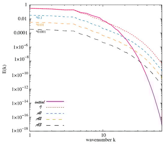
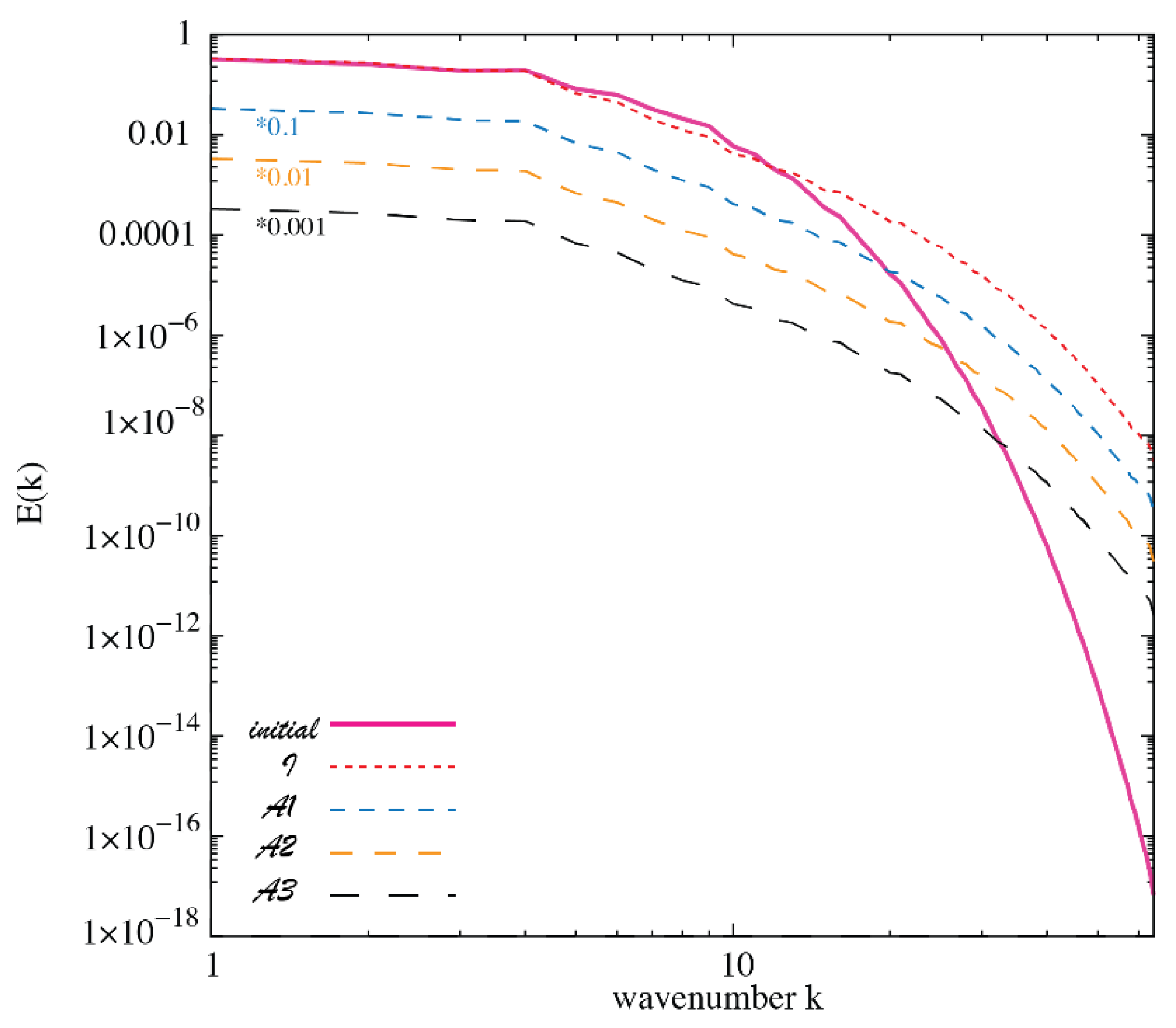
Figure 1.
Comparison of transient kinetic energy spectra for the EDQNM and EDMAC models for the runs in Table 2 at the initial () and final times ().
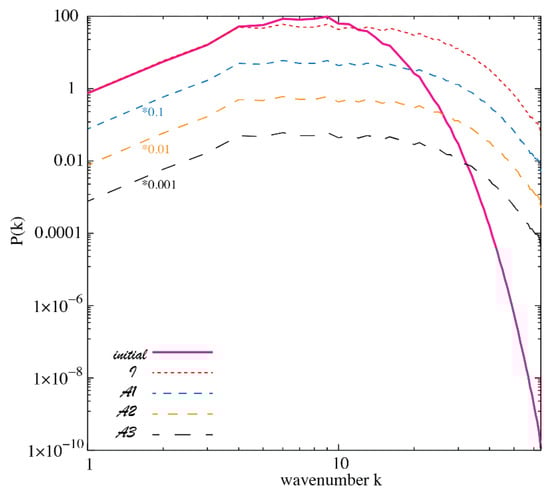
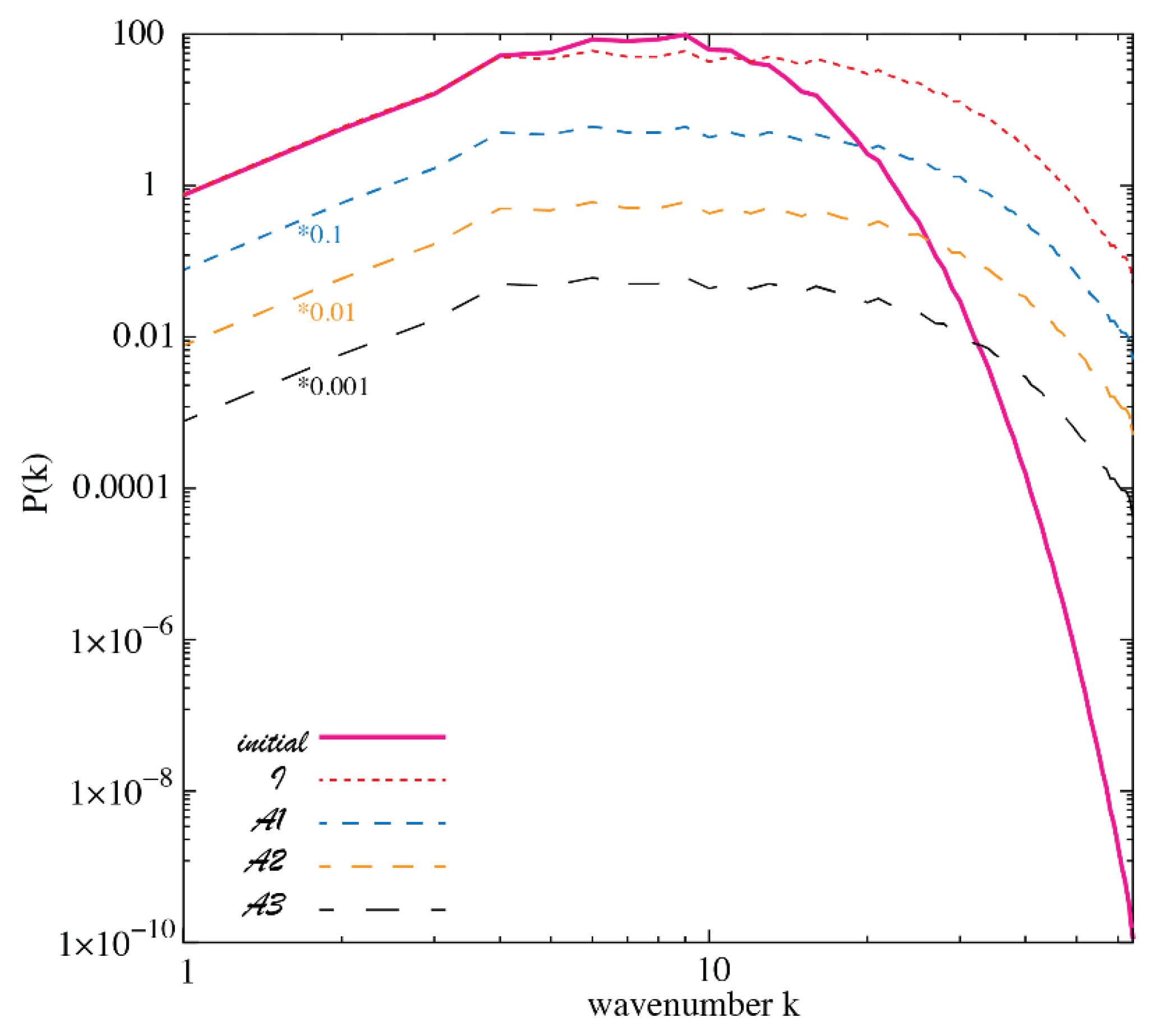
Figure 2.
As in Figure 1 for the palinstrophy spectra .
The inclusion of the large-scale mean flow , corresponding to a dimensional value of , in the anisotropic run with the EDMAC model increases the evolved Reynolds number slightly and decreases the evolved skewness more. Thus, Rossby waves, in the presence of the large-scale flow, make the turbulence more Gaussian.
Thus, in these closure integrations, we conclude that the addition of the frequency-dependent damping in the EDMAC model does not greatly change the results compared with the EDQNM. This is the case for the strength of the eddy damping used in the displayed results. We have also checked that applies equally for strengths of down to 0.01. As is increased to larger values, the frequency-dependent contribution to the eddy damping becomes smaller and the damping experienced by the EDMAC is closer to that of the EDQNM. While the EDQNM closure remained stable for the anisotropic run , this cannot always be guaranteed for the EDQNM, but it can for the EDMAC model under the conditions determined in Section 8 and Appendix B.
11. Discussion and Conclusions
The theoretical development of the Eddy Damped Markovian Anisotropic Closure (EDMAC) has been presented for anisotropic turbulence interacting with Rossby waves in the presence of advection by a large-scale mean flow. The EDMAC generalizes the Eddy Damped Quasi Normal Markovian (EDQNM) to a form that is realizable in the presence of transient waves. We have documented the equations for two-dimensional turbulence interacting with Rossby waves and a large-scale flow in physical space and in discrete Fourier spectral space.
11.1. Theoretical Results
The development of the EDMAC model has then proceeded in a number of steps requiring the formulation of generalized non-Markovian and Markovian closures.
11.1.1. Generalized Non-Markovian Closures
Firstly, renormalized perturbation theory has been employed to construct a generalization of the non-Markovian Direct Interaction Approximation (DIA) closure with additional eddy damping and nonlinear noise terms that depend on the Doppler shifted Rossby wave frequencies. Associated generalized Self Consistent Field Theory (SCFT) and Local Energy-Transfer Theory (LET) closures have also been introduced. The next step has been to slightly simplify these non-Markovian closures to abridged forms in which the large-scale mean flow is regarded as slowly varying in the time history integrals.
11.1.2. Markovian Anisotropic Closures
Markovian Anisotropic Closures (MACs) have then been developed by employing any of three forms of the Fluctuation Dissipation Theorem in Equation (4). This simplifies the time history integrals to the extent that their effects can be encapsulated in two relaxation functions that can also be determined by ordinary Markovian differential equations. While the MACs are more efficient for long time integrations than the non-Markovian closures, the calculation of the relaxation functions through differential equations is a considerable overhead compared with the analytical forms that are used for the EDQNM and established here for the EDMAC.
11.1.3. Realizable Eddy Damped Markovian Anisotropic Closure
The EDMAC has been derived from the MAC employing the current-time Fluctuation Dissipation Theorem (FDT) in Equation (1). Further simplification of the relaxation functions has been achieved by making the Markov approximation that the generalized dissipation functionals are slowly varying in the time history integrals, as for the EDQNM [1]. The consequent EDMAC model has the same eddy damping term as in the EDQNM that parameterizes turbulent mixing [1,2,50,51], but also has a frequency-dependent damping, which ensures the realizability of the EDMAC in the presence of transient waves. The strength of the frequency dependent damping has been determined under the assumption of small amplitude waves, again based on renormalized perturbation theory. More generally, the strength may be specified empirically, and sufficient conditions on the frequency-dependent damping that ensure realizability of the EDMAC have been determined.
11.1.4. Generalizations of the Eddy Damped Markovian Anisotropic Closure
We have considered the relationships between EDQNM and EDMAC models for anisotropic turbulence interacting with transient waves for systems involving higher order nonlinearity than quadratic and in higher dimension than two. The conditions that ensure that the real part of the EDMAC relaxation function is again positive semi-definite have been determined.
11.2. Numerical Closure Calculations
In this largely theoretical paper, we have also reported in detail four integrations of the closures for rapidly evolving turbulence. They have been performed for isotropic 2D turbulence, for anisotropic turbulence with Rossby waves with and without the frequency-dependent damping, and for anisotropic turbulence with Rossby waves and large-scale mean flow and frequency-dependent damping. In these numerical experiments, with empirical parameter in Equation (72), the results of the evolved simulations with EDQNM and EDMAC turn out very similar to each other with little effect on one-dimensional spectra. This is also so for smaller down to , while for larger , the frequency-dependent drain becomes smaller and the total drain in the EDMAC approaches that of the EDQNM.
11.3. Conclusions and Future Prospects
The realizability of the EDMAC in the presence of waves at little or no extra computational cost over the EDQNM should make it attractive provided the additional frequency-dependent damping does not change the broad properties of the numerical integrations with the closures. We have noted, in Section 9, the prospects for generalizing the realizable EDMAC model to higher dimensions and different physical systems, including with higher-order nonlinearity. In future studies, we plan to explore the performance of the EDMAC model in various settings. Also, we aim to formulate and study the performance of a similar inhomogeneous closure, the Eddy Damped Markovian Inhomogeneous Closure (EDMIC) [45], generalized to be realizable for turbulence interacting with transient Rossby waves.
Author Contributions
Conceptualization, J.S.F. and T.J.O.; methodology, J.S.F.; formal analysis, J.S.F.; numeric implementation, T.J.O. and J.S.F.; investigation, J.S.F. and T.J.O.; writing—original draft preparation, J.S.F.; writing—review and editing, J.S.F. and T.J.O.; supervision, J.S.F.; project administration, J.S.F.; funding acquisition, T.J.O. All authors have read and agreed to the published version of the manuscript.
Funding
T.J.O. was funded by CSIRO Environment.
Conflicts of Interest
The authors declare no conflicts of interest.
Correction Statement
The changes include updating or adding prepositions in the abstract, Section 1 and Section 3, updates to Equations (47), (61), (85), (A15), (A16), (A19) and (A21), and updating the format of Reference 13. These changes do not affect the scientific content of the article.
Appendix A. Renormalized Perturbation Theory
The aim of this Appendix is to provide motivation for the modified form of the eddy damping used for the realizable EDMAC model. We begin by expanding in a perturbation series where, from Equations (11), (16) and (17),
That is,
where, in both Equations (A1) and (A2), we have introduced the bookkeeping small parameter that will be set to unity after the renormalization process.
In Equation (A1), is the Doppler shifted Rossby wave frequency defined in Equation (13). We note that can also be written in the form:
where the interaction coefficients are defined by
and
Also, we have defined
and
Here, we have been motivated by the study of Frederiksen and O’Kane [47]. There the transformation in Equation (A6), and the suitable definitions of the interaction coefficients in Equations (A4) and (A5) allowed the combination of the equations for the small scales and the large scale flow into a single form. Here, our aim has been to demonstrate that the term involving the Doppler shifted Rossby wave frequency in Equation (A1) is proportional to the interaction coefficients and, as for the other terms multiplying interaction coefficients there, is assumed to be order in the perturbation theory.
From Equations (A1) and (A2), we see that, to zero order in perturbation theory, we have
To first order, we have
Then, the formal solution to Equation (A9) can be written, using the Greens function corresponding to Equation (A8), as follows:
The two-time cumulant can also be expressed in a perturbation series. Here, we consider homogenous turbulence and
To first order in , we have the two-time cumulant contribution
Next, we consider the perturbation expansion for the response function
where is the response function corresponding to Equation (A8) and is the corresponding average. To first order in , we have
We are now able to write down the dynamical equation for the response function to second order in the perturbation parameter :
with . Perturbation expansion of the last term in Equation (A15) is as described in Frederiksen [9]. On renormalizing with and the zero-order terms replaced by the renormalized terms, we have
where the delta function ensures the initial condition and
as also shown in Equation (26). Here the nonlinear damping is given by
as also shown in in Equation (24).
Next, we consider the two-time two-point cumulant equation, which takes the form:
Again, the perturbation expansion of the three-point terms in Equation (A19) is as described in Frederiksen [9]. Finally, renormalizing with and the zero-order terms replaced by the renormalized terms, we have
Here, the bare noise is given in Equation (23) and
as also shown in Equation (27) with given in Equation (A17) and in Equation (A18). The nonlinear noise takes the form:
as also given in Equation (25).
To close the system of equations, we also need the single-time cumulant equation which takes the form:
Here, the single-time cumulant is to be specified as the initial condition.
Appendix B. Langevin Equation Underpinning the EDMAC Model
In this Appendix, we consider the realizability of the EDMAC model for the single-time cumulant in Equation (61), with replacing . The approach follows that of Leith [3] and Herring and Kraichnan [60] in establishing the realizability of the EDQNM. Again, EDMAC can be shown to be realizable by being underpinned by a suitable stochastic model. The EDMAC model can be constructed exactly from the following Langevin equation:
Here,
as in Equation (44), but with:
also displayed in Equation (64), and with replacing . As shown in Equation (83),
In Equation (A24),
the bare random forcing, and:
which determines the nonlinear noise. Equation (A29) contains the independent random variables , where i = 1, 2, or 3, and . Their properties are such that the statistical dynamical closure for the single-time cumulant in Equation (61), but with replacing , is reconstructed. The statistics of the random variables are such that:
with
and
Here, and are Kronecker delta functions, and is the Dirac delta function.
The single-time cumulants , in the EDMAC model, which are determined by Equation (61) but with replacing , are realizable. This follows from the Langevin Equation (A24) provided . Section 8 outlines the demonstration of the positivity of provided . In the inviscid unforced case, the EDMAC equations conserve kinetic energy and enstrophy.
References
- Orszag, S.A. Analytical theories of turbulence. J. Fluid Mech. 1970, 41, 363–386. [Google Scholar] [CrossRef]
- Leith, C.E. Atmospheric predictability and two-dimensional turbulence. J. Atmos. Sci. 1971, 28, 145–161. [Google Scholar] [CrossRef]
- Herring, J.R. Theory of two-dimensional anisotropic turbulence. J. Atmos. Sci. 1975, 32, 2252–2271. [Google Scholar] [CrossRef]
- Lesieur, M. Turbulence in Fluids; Springer: Dordrecht, The Netherlands, 2008. [Google Scholar]
- Kraichnan, R.H. The structure of isotropic turbulence at very high Reynolds numbers. J. Fluid Mech. 1959, 5, 497–543. [Google Scholar] [CrossRef]
- McComb, W.D. The Physics of Fluid Turbulence; Oxford University Press: Oxford, UK, 1990; ISBN 9780198562566. [Google Scholar]
- McComb, W.D. Homogeneous, Isotropic Turbulence: Phenomenology, Renormalization and Statistical Closures; Oxford University Press: Oxford, UK, 2014; ISBN 9780199689385. [Google Scholar] [CrossRef]
- Berera, A.; Salewski, M.; McComb, W.D. Eulerian field-theoretic closure formalisms for fluid turbulence. Phys. Rev. E 2013, 87, 013007. [Google Scholar] [CrossRef] [PubMed]
- Frederiksen, J.S. Renormalized closure theory and subgrid-scale parameterizations for two-dimensional turbulence. In Nonlinear Dynamics: From Lasers to Butterflies, World Scientific Lecture Notes in Complex Systems; Ball, R., Akhmediev, N., Eds.; World Scientific: Singapore, 2003; Volume 1, pp. 225–256. ISBN 9789814486361. [Google Scholar] [CrossRef]
- Sagaut, P.; Cambon, C. Homogeneous Turbulence Dynamics; Springer Nature: Cham, Switzerland, 2018. [Google Scholar]
- Zhou, Y. Turbulence theories and statistical closure approaches. Phys. Rep. 2021, 935, 1–117. [Google Scholar] [CrossRef]
- Frederiksen, J.S.; O’Kane, T.J. Realizable Eddy Damped Markovian Anisotropic Closure for Turbulence and Rossby Wave Interactions. Atmosphere 2023, 14, 1098. [Google Scholar] [CrossRef]
- McComb, D. Jackson R. Herring and the Statistical Closure Problem of Turbulence: A Review of Renormalized Perturbation Theories. Atmosphere 2023, 14, 827. [Google Scholar] [CrossRef]
- Rose, H.A. An efficient non-Markovian theory of non-equilibrium dynamics. Physica D 1985, 14, 216–226. [Google Scholar] [CrossRef]
- Frederiksen, J.S.; Davies, A.G. Dynamics and spectra of cumulant update closures for two-dimensional turbulence. Geophys. Astrophys. Fluid Dyn. 2000, 92, 197–231. [Google Scholar] [CrossRef]
- Frederiksen, J.S.; Davies, A.G. The regularized DIA closure for two-dimensional turbulence. Geophys. Astrophys. Fluid Dyn. 2004, 98, 203–223. [Google Scholar] [CrossRef]
- O’Kane, T.J.; Frederiksen, J.S. The QDIA and regularized QDIA closures for inhomogeneous turbulence over topography. J. Fluid Mech. 2004, 65, 133–165. [Google Scholar] [CrossRef]
- Herring, J.R. Self-consistent-field approach to turbulence theory. Phys. Fluids 1965, 8, 2219–2225. [Google Scholar] [CrossRef]
- Herring, J.R. Self-consistent-field approach to nonstationary turbulence. Phys. Fluids 1966, 9, 2106–2110. [Google Scholar] [CrossRef]
- McComb, W.D. A local energy-transfer theory of isotropic turbulence. J. Phys. A 1974, 7, 632–649. [Google Scholar] [CrossRef]
- McComb, W.D. A theory of time dependent, isotropic turbulence. J. Phys. A 1978, 11, 613–633. [Google Scholar] [CrossRef]
- Cambon, C.; Mons, V.; Gréa, B.-J.; Rubinstein, R. Anisotropic triadic closures for shear-driven and buoyancy-driven turbulent flows. Computers Fluids 2017, 151, 73–84. [Google Scholar] [CrossRef]
- Bowman, J.C.; Krommes, J.A.; Ottaviani, M. The realizable Markovian closure. I. General theory, with application to three-wave dynamics. Phys. Fluids 1993, 5, 3558–3589. [Google Scholar] [CrossRef]
- Carnevale, G.F.; Martin, P.C. Field theoretic techniques in statistical fluid dynamics: With application to nonlinear wave dynamics. Geophys. Astrophys. Fluid Dyn. 1982, 20, 131–164. [Google Scholar] [CrossRef]
- Carnevale, G.F.; Frederiksen, J.S. A statistical dynamical theory of strongly nonlinear internal gravity waves. Geophys. Astrophys. Fluid Dyn. 1983, 23, 175–207. [Google Scholar] [CrossRef]
- Zhou, Y.; Matthaeus, W.H.; Dmitruk, P. Magnetohydrodynamic turbulence and time scales in astrophysical and space plasmas. Rev. Mod. Phys. 2004, 76, 1015–1034. [Google Scholar] [CrossRef]
- Frederiksen, J.S.; Dix, D.R.; Kepert, S.M. Systematic energy errors and the tendency towards canonical equilibrium in atmospheric circulation models. J. Atmos. Sci. 1996, 53, 887–904. [Google Scholar] [CrossRef]
- Holloway, G. On the spectral evolution of strongly interacting waves. Geophys. Astrophys. Fluid Dyn. 1978, 11, 271–287. [Google Scholar] [CrossRef]
- Vallis, G.K.; Maltrud, M.E. On the Generation of Mean Flows and Jets on a Beta Plane and over Topography. J. Phys. Oceanog. 1993, 23, 1346–1362. [Google Scholar] [CrossRef]
- Sukoriansky, S.; Galperin, B. QNSE theory of turbulence anisotropization and onset of the inverse energy cascade by solid body rotation. J. Fluid Mech. 2016, 805, 384–421. [Google Scholar] [CrossRef]
- Galperin, B.; Sukoriansky, S.; Qiu, B. Seasonal oceanic variability on meso- and sub-mesoscales: A turbulence perspective. Ocean Dynam. 2021, 71, 475–489. [Google Scholar] [CrossRef]
- Hu, G.; Krommes, J.A.; Bowman, J.C. Statistical theory of resistive drift-wave turbulence and transport. Phys. Plasmas 1997, 4, 2116–2133. [Google Scholar] [CrossRef]
- Bowman, J.C.; Krommes, J.A. The realizable Markovian closure and realizable test-field model. II. Application to anisotropic drift-wave dynamics. Phys. Plasmas 1997, 4, 3895–3909. [Google Scholar] [CrossRef]
- Kraichnan, R.H. An almost Markovian Galilean invariant turbulence model. J. Fluid Mech. 1971, 47, 513–524. [Google Scholar] [CrossRef]
- Kraichnan, R.H. Inertial ranges in two-dimensional turbulence. Phys. Fluids 1967, 10, 1417–1423. [Google Scholar] [CrossRef]
- Rhines, P.B. Waves and turbulence on a beta-plane. J. Fluid Mech. 1975, 69, 417–443. [Google Scholar] [CrossRef]
- Holloway, G.; Hendershott, M.C. Stochastic closure for nonlinear Rossby waves. J. Fluid Mech. 1977, 82, 747–765. [Google Scholar] [CrossRef]
- Chekhlov, A.; Orszag, S.A.; Sukoriansky, S.; Galperin, B.; Staroselsky, I. The effect of small-scale forcing on large-scale structures in two-dimensional flows. Phys. D 1996, 98, 321–334. [Google Scholar] [CrossRef]
- Galperin, B.; Sukoriansky, S.; Young, R.M.B.; Chemke, R.; Kaspi, Y.; Read, P.L.; Nadejda, D. Barotropic and Zonostrophic Turbulence. In Zonal Jets: Phenomenology, Genesis and Physics; Galperin, B., Read, P.L., Eds.; Cambridge University Press: Cambridge, UK, 2019; pp. 220–237. [Google Scholar] [CrossRef]
- Krommes, J.A.; Parker, J.B. Statistical Closures and Zonal Flows. In Zonal Jets: Phenomenology, Genesis and Physics; Galperin, B., Read, P.L., Eds.; Cambridge University Press: Cambridge, UK, 2019; pp. 309–331. [Google Scholar] [CrossRef]
- Galperin, B.; Read, P.L. (Eds.) Zonal Jets: Phenomenology, Genesis and Physics; Cambridge University Press: Cambridge, UK, 2019; pp. 309–331. [Google Scholar] [CrossRef]
- Cabanes, S.; Gastine, T.; Fournier, A. Zonostrophic turbulence in the subsurface oceans of the Jovian and Saturnian moons. Icarus 2024, 415, 116047. [Google Scholar] [CrossRef]
- Frederiksen, J.S. Strongly nonlinear topographic instability and phase transitions. Geophys. Astrophys. Fluid Dyn. 1985, 32, 103–122. [Google Scholar] [CrossRef]
- Frederiksen, J.S.; O’Kane, T.J. Markovian inhomogeneous closures for Rossby waves and turbulence over topography. J. Fluid Mech. 2019, 858, 45–70. [Google Scholar] [CrossRef]
- Frederiksen, J.S.; O’Kane, T.J. Statistical Dynamics of Mean Flows Interacting with Rossby Waves, Turbulence, and Topography. Fluids 2022, 7, 200. [Google Scholar] [CrossRef]
- Frederiksen, J.S. Subgrid-scale parameterizations of eddy-topographic force, eddy viscosity and stochastic backscatter for flow over topography. J. Atmos. Sci. 1999, 56, 1481–1494. [Google Scholar] [CrossRef]
- Frederiksen, J.S.; O’Kane, T.J. Inhomogeneous closure and statistical mechanics for Rossby wave turbulence over topography. J. Fluid Mech. 2005, 539, 137–165. [Google Scholar] [CrossRef]
- Frederiksen, J.S. Statistical dynamical closures and subgrid modeling for QG and 3D inhomogeneous turbulence. Entropy 2012, 14, 32–57. [Google Scholar] [CrossRef]
- Frederiksen, J.S. Quasi-diagonal inhomogeneous closure for classical and quantum statistical dynamics. J. Math. Phys. 2017, 58, 103303. [Google Scholar] [CrossRef]
- Pouquet, A.; Lesieur, M.; Andre, J.C.; Basdevant, C. Evolution of high Reynolds number two-dimensional turbulence. J. Fluid Mech. 1975, 72, 305–319. [Google Scholar] [CrossRef]
- Herring, J.R.; Schertzer, D.; Lesieur, M.; Newman, G.R.; Chollett, J.P.; Larcheveque, M. A comparative assessment of spectral closures as applied to passive scalar diffusion. J. Fluid Mech. 1982, 124, 411–437. [Google Scholar] [CrossRef]
- Cambon, C.; Jacquin, L. Spectral approach to non-isotropic turbulence subject to rotation. J. Fluid Mech. 1989, 202, 295–317. [Google Scholar] [CrossRef]
- Rose, H.A.; Sulem, P.-L. Fully developed turbulence and statistical mechanics. J. Phys. 1978, 39, 441–484. [Google Scholar] [CrossRef]
- Clark, D.; Ho, R.D.J.G.; Berera, A. Effect of spatial dimension on a model of fluid turbulence. J. Fluid Mech. 2021, 912, A40-1–29. [Google Scholar] [CrossRef]
- Nazarenko, S. Wave Turbulence; Springer Lecture Notes in Physics; Springer: Berlin/Heidelberg, Germany, 2011; ISBN 978364215942. [Google Scholar]
- Dyachenko, A.; Newell, A.C.; Pushkarev, A.; Zakharov, V.E. Optical turbulence: Weak turbulence, condensates and collapsing fragments in the nonlinear Schrodinger equation. Phys. D 1992, 57, 96–160. [Google Scholar] [CrossRef]
- Blagoev, K.B.; Cooper, F.; Dawson, J.F.; Mihaila, B. Schwinger-Dyson approach to nonequilibrium classical field theory. Phys. Rev. D 2001, 64, 125033. [Google Scholar] [CrossRef]
- Berges, J.; Sexty, D. Bose-Einstein condensation in relativistic field theories far from equilibrium. Phys. Rev. Lett. 2012, 108, 161601. [Google Scholar] [CrossRef] [PubMed]
- Herring, J.R.; Orszag, S.A.; Kraichnan, R.H.; Fox, D.G. Decay of two-dimensional homogeneous turbulence. J. Fluid Mech. 1974, 66, 417–444. [Google Scholar] [CrossRef]
- Herring, J.R.; Kraichnan, R.H. Statistical Models and Turbulence. In Lecture Notes in Physics: Proceedings of the Symposium Held at the University of California, San Diego, CA, USA, 15–21 July 1971; Ehlers, J., Hepp, K., Weidenmuller, H.A., Eds.; Springer: Berlin/Heidelberg, Germany, 1972; pp. 148–194. [Google Scholar]
Disclaimer/Publisher’s Note: The statements, opinions and data contained in all publications are solely those of the individual author(s) and contributor(s) and not of MDPI and/or the editor(s). MDPI and/or the editor(s) disclaim responsibility for any injury to people or property resulting from any ideas, methods, instructions or products referred to in the content. |
© 2024 by the authors. Licensee MDPI, Basel, Switzerland. This article is an open access article distributed under the terms and conditions of the Creative Commons Attribution (CC BY) license (https://creativecommons.org/licenses/by/4.0/).