Abstract
Induction motors (IMs) must meet high reliability and safety standards in mission-critical applications, such as electric vehicles (EVs), where sensorless control strategies are fundamental. However, sensorless rotor speed estimation demands improvements to overcome filtering distortions, tuning complexities, and sensitivity to IM model mismatch. Algebraic methods offer inherent filtering capabilities and design flexibility to address these challenges without introducing additional dynamics into the control system. The objective of this paper is to provide an algebraic estimation strategy that yields an accurate rotor speed estimate for sensorless IM control. The strategy includes an algebraic estimator with single-parameter tuning and inherent filtering action. We propose an EV case study to experimentally evaluate and compare its performance with a typical drive cycle and a dynamic torque load that emulates a small-scale EV power train. The algebraic estimator exhibited a signal-to-noise ratio (SNR) of 43 dB. The closed-loop experiment for the EV case study showed average tracking errors below 1 rad/s and similar performance compared to a well-known sensorless strategy. Our results show that the proposed algebraic estimation strategy works effectively in a nominal speed range for a practical IM sensorless application. The algebraic estimator only requires single-parameter tuning and potentially facilitates IM model updates using a resetting scheme.
1. Introduction
Induction motors (IMs) demand continuous improvement in reliability and safety in various industries, including automotive, manufacturing, and renewable energy. In electric vehicle (EV) systems, for example, IMs have been used as mission-critical components with historical advantages in cost-effectiveness, reduced maintenance, and high-performance efficiency [1]. However, IM controllers are vulnerable to mechanical speed sensor faults, leading to potentially hazardous conditions. Sensorless control techniques have become indispensable tools for ensuring redundancy and fault tolerance, offering a viable alternative that complies with stringent reliability and safety standards [2].
Research on sensorless techniques for IMs is an active topic with contributions that aim to alleviate persistent challenges and develop innovative schemes [3]. Compared to signal injection alternatives, model-based speed estimation methods have shown advantages and multiple perspectives with increasing development [4]. Remarkable examples of model-based techniques include model reference adaptive systems (MRASs) in [5,6], adaptive flux observers (AFOs) in [7], extended Kalman filters (EKFs) in [8], sliding mode observers (SMOs) in [9], full or reduced-order state observers (SOs) in [10,11], artificial neural networks (ANNs) in [12], and specialized stator flux estimators in [13,14].
Between the different approaches, there is a joint effort to face the multiple challenges of sensorless control and speed estimation. Problems include low/zero speed operation, tuning complexities, and IM model sensitivities. For closed-loop techniques, such as MRASs, there are also stability concerns [5], training requirements [12], and computational complexities [8]. For open-loop techniques, such as flux estimators, filtering stages affect estimator performance and floating-point overflow when performing numerical integration [10,11]. However, there is an unexplored potential in the adaptation of an algebraic methodology for the rotor speed estimation problem in sensorless IM control.
Algebraic methods have shown beneficial properties in developing an open-loop alternative for speed estimation. Since their theoretical foundation in works including [15,16], further developments and experimental results have shown advantages in design flexibility, inherent filtering capabilities, and high performance for state estimations. For example, a robust framework for an extensive range of applications, especially estimation problems in control, is presented in [17]. It has been used successfully to identify the parameters of the IM model in [18] and to estimate disturbances in [19].
Some notable strengths of the algebraic framework in [17] include design flexibility, faster estimations, statistically independent noise treatment schemes, and reinitialization techniques to manage integral overflow. Some challenges include computational complexities and the disconnection from classical asymptotic convergence, Lyapunov stability theory, and classical observability. However, the major technological breakthrough on the available processors and non-standard analysis with numerical indices provide tools to overcome those obstacles. Therefore, it is a technique that can face some challenges of the IM rotor speed estimation problem.
This paper aims to provide an algebraic estimation strategy that yields an accurate rotor speed estimate for sensorless IM control. Our proposal is described in three major components. First, we develop an algebraic estimator with single-parameter tuning and inherent filtering action that adapts the concepts and techniques in [17,19]; see Section 2. An equation is derived from a classical IM model to obtain a relation between the available data (voltage/current measurements and model parameters) and the unknown data (rotor speed and rotor-flux initial conditions). The rotor speed is locally approximated to a constant considering sufficiently short time intervals defined with sliding-window integrals. An algebraic pseudoinverse-like procedure is proposed to update that local approximation continuously, hence providing an algebraic estimate for the IM rotor speed.
Second, the analysis and tools required to deal with critical experimental conditions for our algebraic estimation strategy are presented. We introduce a current derivative estimator in Section 2.1.3 to simplify the algebraic estimator structure and reduce the adverse effects of filters. Later, in Section 2.1.5, a numerical condition analysis sets clear guidelines for the practical selection of sliding-window widths. We use QR factorization to provide numerically stable inverse matrix calculations on a microprocessor. Lastly, in Section 2.2, our proposal includes an integral resetting scheme to eliminate floating-point overflow problems and potentially facilitate integration with online IM model adaptation mechanisms.
Third, the experimental evaluation of our algebraic speed estimation strategy with an electric vehicle case study is introduced in Section 3. Control and estimation algorithms are implemented using real-time simulation techniques. We performed tests in a closed-loop IM drive control system using a laboratory setup to emulate a small-scale EV power train. So, the experiments use typical EV load torque and speed conditions with the Urban Dynamometer Driving Schedule (UDDS) of the Environmental Protection Agency of the United States (EPA).
Therefore, the main contribution of this article is the development of a rotor speed algebraic estimation strategy considering key practical implementation requirements for sensorless IM control. Our proposal differs from classical algebraic approaches in [17,19], combining a derivative estimator, sliding-window integrals, and a resetting scheme to achieve a simpler and more robust structure. The strategy only requires tuning one additional parameter, the sliding-window width. This parameter is directly related to the performance/filtering specifications, and our experiments confirmed that it can be adjusted to obtain estimations with an SNR of 43 dB. Using the resetting scheme in Section 2.2, the estimator design is flexible and easier to integrate with flux estimators, control strategies, and parameter adaptation mechanisms. We provide detailed procedures and results for a small-scale electric vehicle case study in Section 4, showing that our strategy yields adequate tracking performance for sensorless control applications. The algebraic estimator works within a nominal speed range, with a high SNR and low estimation errors under experimental conditions. A further discussion of our results and future work is presented in Section 5.
2. An Algebraic Estimation Strategy for the IM Rotor Speed
This section presents our algebraic estimator strategy for the IM rotor speed . Its two fundamental components are illustrated with the block diagram in Figure 1. The first component is the algebraic estimator. We use two copies (main and auxiliary) to provide an uninterrupted estimate of the speed with , . The second component is an integral resetting scheme to prevent numerical overflows inside the algebraic estimator calculations and allow online parameter updates. A resetting logic governs the execution of the main and auxiliary copies with the reset signals , , and the selector signal . Thus, a valid speed estimate is available even during a reset or an online parameter update of our algebraic estimator.
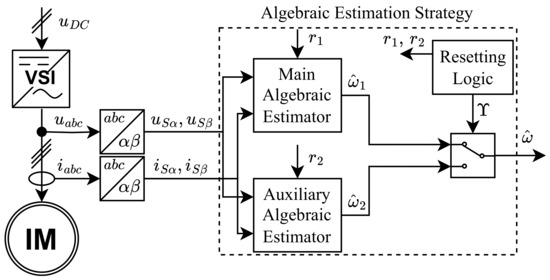
Figure 1.
Block diagram of the algebraic estimation strategy.
A detailed description of each component is presented in the following subsections.
2.1. Algebraic Estimator
The objective of this component is to provide an estimation for using only the available electrical measurements, i.e., the stator voltages and currents , and the structure of the IM dynamic model with its corresponding parameters.
2.1.1. Base Equation
The selection of the IM model and its reference frame is our first step. To keep the structure simple, we use the classical two-phase model with equivalent rotor flux linkages , within a fixed stator reference frame [20],
The machine parameters include the moment of inertia J, the number of pole pairs , the two-phase equivalent rotor and stator resistance , , rotor and stator inductance , , and magnetizing inductance , where . This model structure presents highly coupled nonlinear dynamics, and its parameters can change over time. The load torque is unknown, and there is no practical way to measure the flux states , . The electrical measurements have noise and DC offsets.
Our goal here is to devise an equation from the model that helps to address those challenges and develop an algebraic estimation for the rotor speed . So, we begin with some algebraic manipulations over (5) and (6). This allows us to exclude the mechanical dynamics in (2), eliminate the influence of , ignore the J parameter, and obtain the equivalent rotor flux and its derivatives using only the stator current and voltage measurements.
It is direct from (5), (6) that the flux derivatives can be obtained as:
An integral re-constructor for the flux is then obtained from an initial time until the current time t, using (7) and (8):
Equation (11) is valuable as it relates the rotor speed along with and , expressions that can be calculated from the available measurements and the electrical parameters. However, this equation demands additional manipulations to adjust its structure for an algebraic estimation. requires a current derivative estimation, and we must deal with the initial conditions associated with the rotor flux.
2.1.2. A Locally Valid Speed Approximation
We now prepare (11) for the algebraic estimation with inspiration from the concepts presented in [17,19]. For sufficiently short time intervals defined with a sliding-window width T, the rotor speed can be considered as a signal which is locally represented using an m-order Taylor polynomial approximation with real coefficients , i.e.,
Depending on the local period of the approximation, a sufficiently high order m is required for to remain valid. However, a small m significantly reduces complexity for the algebraic estimator. Thus, inspired by the classic and effective zero-order hold method used for discretization, our proposal also works using a sufficiently short time window where even the simplest approximation provides a valid result, i.e.,
closely represents the rotor speed during a sufficiently small sliding-window width T, and will be continuously updated with the faster sample time where the algebraic estimation will be computed.
2.1.3. Current Derivative Estimator in DQ Reference Frame
Classical algebraic methods avoid derivatives by means of integration, but this application greatly benefits from a simpler structure. Therefore, we use a stator-current-oriented DQ reference frame for the derivative calculation required in (12) for . This process reduces the classical delay and distortion introduced by filters handling experimental noise during derivative calculations.
Using space vector notation,
where , , and j is the imaginary unit. The DQ stator current is oriented with resulting in , and . Within this DQ reference frame, the stator current derivatives in the stationary reference frame are obtained as
The derivatives for and are estimated using a classical low-pass filter approximation described with a transfer function , where is the cutoff frequency, and utilizing the notation
2.1.4. The Algebraic Procedure for State Estimation
It is now possible to establish an equation for the algebraic estimation. We use the constant speed approximation and the available estimation for the current derivative in and we address the unknown rotor flux initial conditions as an additional constant parameter requiring estimation, so (11) can be written as,
With (19), it is now possible to perform an estimation procedure inspired by algebraic methodology. We transform a nonlinear state estimation problem into a continuous estimation of constant parameters. So, our new objective is to devise an algebraic structure to continuously estimate the constant approximation of the rotor speed and a linear combination between and the initial conditions of the rotor flux, i.e., .
First, we write (19) using vectorial notation for further simplicity,
where,
with representing the unknown parameters and , the expressions that can be calculated from the electrical measurements , , , and .
Assuming that the machine parameters , , , , , and remain constant during a local time span of value T, an algebraic procedure, similar to the pseudoinverse calculation, is used to provide the continuous estimations of the unknown parameters . The terms in (20) are pre-multiplied by , i.e., the vector transpose of ,
A key difference from classical algebraic methods is then applied. With an integral over a sliding-window of width T that defines our local time frame,
we soon show that the matrix at the left hand side is non-singular. So, a continuous estimate for vector could be obtained directly with where
a result that is equivalent to an application of the Least Squares Method; see details in [19].
However, experimental errors and parameter inaccuracy affect the matrix and the vector during microprocessor calculations with limited numerical precision. To attenuate some of its adverse effects, we choose the QR factorization algorithm to solve (24) and the calculation of any inverse matrices required in the simulations and experiments presented in this work. Calculations with QR factorization provide a balance between reduced sensitivity to numerical perturbations and computational complexity, something critical for real-time executions [21].
Therefore, the online algebraic estimation for the rotor speed is achieved using
where is continuously and automatically updated on account of the sliding-window integrals in (24), its solution with the QR factorization, and the sampling period for the algorithm execution in the microprocessor. A block diagram for this algebraic estimator is shown in Figure 2.
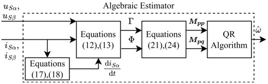
Figure 2.
Block diagram of the algebraic estimator.
2.1.5. Sliding-Window Width Tuning and Numerical Analyses
Our algebraic strategy demands a careful numerical analysis due to the structure of (24). For example, the numerical condition of the matrix is critical for obtaining an accurate and reliable estimate. We directly analyze this matrix for singular or nearly singular situations where the numerical condition worsens. The matrix is symmetric by construction. So, if it is also positive definite, is non-singular. We examine this by considering the scalar , where is an arbitrary non-zero and constant vector over T, i.e.,
It is ensured that . So, we focus on the case . It is only possible if the vector components in are linearly dependent during a time interval of width T, i.e.,
holds during a time interval of width T. Thus, if is not constant during a time interval of width T, it is also warrantied that , and the matrix is non-singular for every .
We further analyze to verify that our previous condition is coherent under typical IM operation conditions. With the definitions in (10) and (13), it is clear that . Under steady-state conditions, the magnetic rotor flux component could remain constant. However, sinusoidal behavior generally dominates with a fundamental angular frequency , and holds for most practical IM applications. Indeed, is the classical unobservable condition of zero excitation frequency (see [22]), and it agrees with our numerical condition requirements.
Finally, we establish tuning criteria for the sliding-window width T. Its definition is critical for complying with our local constant speed approximation in (15), the numerical condition, and the noise-filtering action [19]. If a value of is used, low-noise-filtering action results, and can be approximated nearly to a constant over T, i.e., it results in a nearly singular situation with a poor numerical condition. If a value of is used, the noise-filtering action result is excessive and, more importantly, the approximation (15) starts to lose validity. Choosing a value slightly higher than the period at nominal stator frequency is helpful for most applications.
Our proposed tuning criteria are confirmed during our experiments in Section 4. The plot in Figure 3 shows an evaluation of the SNR while tuning the sliding-window width T for our case study. It includes the calculation of the SNR for the estimations obtained using the algebraic estimator and the SNR obtained using the encoder measurements as a reference. The algebraic estimator was evaluated for multiple T values. The values of s performed poorly with an SNR around 30 dB. As T increased, the SNR improved and reached the same performance as the optical encoder at with 47 dB. The SNR continues to increase with a logarithmic trend, but the estimation error metrics also increased. For our case study with Hz, algebraic estimator tuning revealed a value , resulting in an SNR close to that obtained using an encoder measurement.
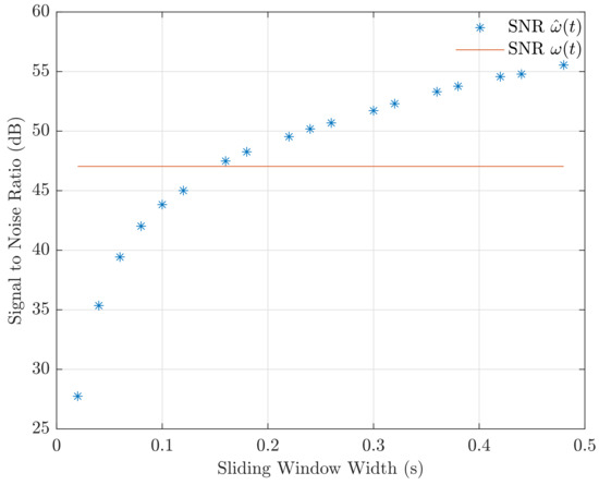
Figure 3.
SNR evaluation for different sliding−window width (T) using experimental data. The SNR of the experimental encoder measurement (orange line) and SNR of the algebraic estimation (blue *).
2.2. Integral Resetting Scheme
The algebraic estimator has expressions for and that involve pure integration of the stator voltages and currents. These quantities are affected with DC offsets due to sensor calibration issues, inverter nonlinearities, and some normal operating conditions of the IM. So, integration is generally avoided for sensorless schemes, and complex low-pass filters or some novel proposals with DC offset compensation are used instead of pure integration; see [13,14].
In contrast, our algebraic estimator uses a simpler resetting scheme to prevent precision degradation and numerical overflows. This scheme is not present in classical algebraic methods, but [19] shows that it is a valuable tool. Different from [19], our scheme does not require timelines, and it is also helpful in facing model mismatch effects. This is due to the zero-order approximation (14) and the easier integration with online parameter updating schemes during the reset events.
As depicted in Figure 1 this scheme requires two steps. First, the algebraic estimator, a main, and an auxiliary block are duplicated. Furthermore, second, a resetting logic block is designed that sends suitable resetting signals , and a selection signal .
The resetting logic is illustrated with its signals in Figure 4. The rising edges , represent the resetting points for the main and auxiliary blocks, respectively. The main estimator is reset with a period in accordance with the numerical hardware limitations or an online policy for parameter updates. The auxiliary estimator is only activated units of time before each resetting action over the main estimator, and corresponds to the minimum time required for the estimators to converge. The signal selects the main one most of the time, except for periods where its resetting takes place and selects the auxiliary estimator.
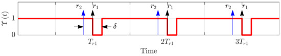
Figure 4.
Signals of the resetting logic.
Both estimators, the main and auxiliary, are simultaneously active during small time intervals due to the almost instantaneous nature of the algebraic estimator. Therefore, this design reduces the algorithm’s complexity, effectively avoids numerical overflows, and enables the integration with online parameter updates.
3. An Electric Vehicle Case Study
An electric vehicle (EV) with an IM-based drivetrain is selected to study the algebraic speed estimation strategy in a practical application. This analysis uses a simplified model of the vehicle mechanics and aerodynamics described as a load torque and load inertia attached to the IM. A one-degree-of-freedom vehicle body under longitudinal motion conditions is considered; see Figure 5. The EV’s weight is assumed to be uniform over the wheels, with its center of mass located in the center of the vehicle along the wheel axes. The EV drivetrain topology is assumed to be located to the rear with a single IM drive powering an ideal fixed gearbox and differential connecting the axle and its wheels.
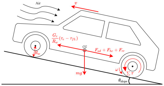
Figure 5.
Forces acting on a longitudinal vehicle model.
3.1. Electric Vehicle Model
We use a simplified vehicle model, similar to approaches found at [23,24], where the following forces are frequently associated with the total tractive load.
It includes the aerodynamic drag force associated with the vehicle body moving a mass of air. It depends on the air density , the drag coefficient , the vehicle frontal area , and the direction and magnitude of the EV linear speed v.
A hill-climbing force when the vehicle mass m is moving through an inclined plane with a slope defined by the angle under the influence of earth’s gravity g.
Moreover, a rolling resistance force due to the friction interaction between the wheels and the road surface is described with a dynamic friction coefficient and acting against the movement of the vehicle.
The motor load torque is then defined by the motor shaft friction load and the simplified total tractive load considering the wheel radius and the fixed gear ratio .
The updated mechanical dynamic model for the IM drive in the EV is thus described with
where is the electrical torque produced by the IM. the total inertia of the EV, including the motor inertia J, the wheel inertia associated with the wheel mass , the shaft inertia associated with the vehicle mass, and the slip of the wheel , assumed to be zero under ideal road-tire conditions with a high adhesion coefficient.
3.2. Preliminary Transient Simulations and Parameter Sensitivity Analysis
This section evaluates fast transients and the sensitivity of the parameters , with simulations. Before experimental studies, these results are obtained for our proposed algebraic strategy and the MRASCC estimator proposed by [6] and further described in Section 4.2 for our comparison purposes. The values and were used for simulations using the MRASCC estimator.
We performed multiple simulations to cover fast transients for high-, medium-, and low-speed ranges. The simulations considered noise and DC offset components in the stator voltages and currents, like those obtained with our experiments. The transients cover zero-crossing and reverse-speed conditions with 3 s steps of nominal torque load applied and released during steady state. The results are presented in Figure 6 and Figure 7.
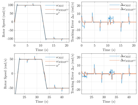
Figure 6.
Simulations for IM algebraic and MRASCC sensorless FOC facing fast high- and medium-speed ranges.
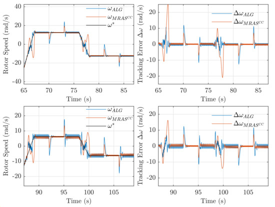
Figure 7.
Simulations for IM algebraic and MRASCC sensorless FOC facing fast low- and ultra-low-speed ranges.
Both strategies show similar performance, with significant tracking errors only present during transient events. The results are also consistent with our further experimental observations. The algebraic strategy presents more significant transient errors, but the MRASCC presents larger transient errors for low-speed ranges.
The parameter sensitivity is ascertained for the IM parameter mismatch between for and for . The mismatch is introduced during 3 s at nominal torque load and 3 different steady-state speed levels that cover a significant portion of the nominal speed range from 12.5 to 100 rad/s.
The results in Figure 8 show a significant steady-state error as a result of the mismatch, consistent for both estimation approaches. The situation is different for the mismatch. The simulations show a more sensitive response to this parameter, particularly for the overestimation of . Both the algebraic and MRASCC techniques present potentially unbounded behavior, with the MRASCC error increasing faster for low speeds.
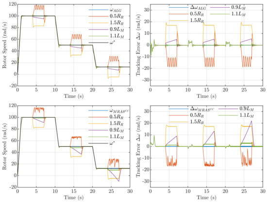
Figure 8.
Simulations for IM algebraic and MRASCC sensorless FOC facing parameter mismatch.
4. Experimental Results and Comparison
This section details the experimental setup, its configurations, and the results for two experiments. An experiment validates our algebraic estimation strategy for the EV case study. Another experiment implements the well-known MRASCC sensorless strategy proposed in [6] for comparison purposes. We use a low-power setup using an IM coupled to a DC Generator (DCG). The test bench is integrated with real-time simulation equipment to implement algorithms. The tests are executed in closed-loop using PI control and emulating typical EV speed and torque conditions. The results exhibit small tracking error bounds for both tests and confirm the effectiveness of the algebraic speed estimator for sensorless applications.
Our experimental setup supplies a 100 W IM from a filtered VSI controlled with conventional PWM. The IM is mechanically coupled to a DCG for small-scale load torque emulation of the EV powertrain. To provide load torque for low or zero speeds (limited to 0.3 Nm), the DCG is connected in series to a DC voltage source (30 V). Both elements supply a resistive load (30 ) through a PWM-controlled DC-DC converter. Isolated current and voltage transducers with instrumentation circuits (analog amplification and filters) provide the electrical measurements and for the IM and for the DCG. Optical incremental encoders with 2500 ppr provide an angular speed measurement used for load torque emulation and comparison of speed estimations. The control and estimation algorithms are implemented in the Matlab/Simulink environment and deployed to xPC-Target-based platforms for real-time simulation with a sample time of 0.1 ms. The xPC-Target computers are equipped with Intel Pentium D processors, National Instruments data acquisition (PCI-6024e) and counter (PCI-6602) cards. A picture of the setup is given in Figure 9, and a circuit diagram is shown in Figure 10. The IM parameters are obtained through classic identification methods and are presented in Table A1.
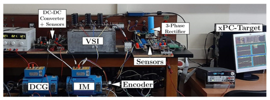
Figure 9.
Picture of the laboratory setup.
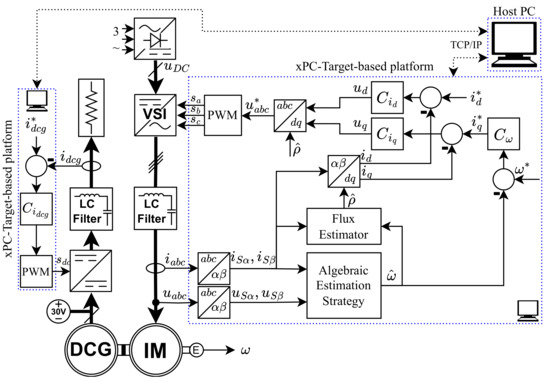
Figure 10.
Experimental setup circuit diagram and IM algebraic sensorless FOC block diagram.
4.1. Experimental Validation of the Algebraic Estimation Strategy
This first validation test is performed with an IM under conditions of sensorless field-oriented control (FOC), PI controllers , and our speed estimation strategy. The DCG provides our load torque emulation using a PI current controller . IM current control loops are designed with 233 rad/s bandwidth (, ) and speed control loop with 4 rad/s bandwidth (, ). Our algebraic estimator is configured with a window width s and a reset time s. The cutoff frequency rad/s is selected for the low-pass filters in the current derivative estimator.
The algebraic estimation strategy was evaluated with an UDDS speed command that is used as an EPA-standard procedure for vehicle testing. During this experiment, the DCG current is controlled to provide a load torque emulation that implements the vehicle model in Section 3.1. The results in Figure 11 show a dB for the algebraic speed estimation . This value is close to the dB obtained from the encoder speed measurements . The tracking error defined has an average value lower than rad/s or p.u., except for transients during starting and braking operations. The electromagnetic torque and the field-oriented DQ currents , confirm the proper operation of the sensorless controller even under highly varying load torque conditions.
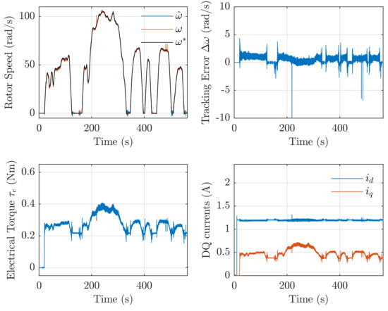
Figure 11.
Experimental results for UDDS speed command with algebraic sensorless FOC.
4.2. Experimental Implementation of MRASCC Sensorless and Comparison Metrics
This section presents a brief description and implementation of the stator-current-based MRASCC estimator presented in [6] along with comparison points regarding our algebraic estimation strategy. The reference model is established with the induction motor within the stationary reference frame. This represents a starting point similar to the one used in our proposal in Section 2.1.1, where we obtain the base equation of the estimator. However, the MRASCC proposal is proposed with a completely different methodology described by the block diagram in Figure 12.
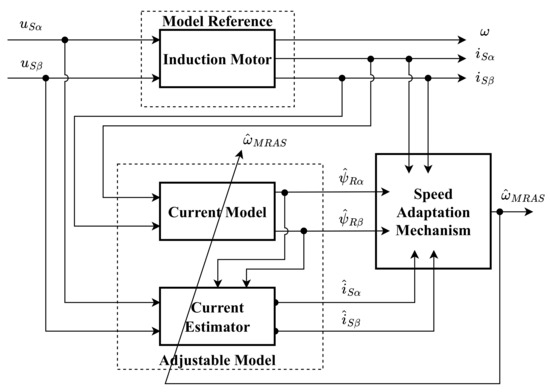
Figure 12.
Block diagram for the stator-current-based MRASCC [6].
The adaptive model is built with the equations associated with the rotor flows,
and those associated with the stator currents and rotor fluxes,
The MRASCC strategy proposed in [6] uses an adaptation mechanism based on the error between the stator current measurements and the current estimate obtained with (37), i.e., , defined with the expression
This mechanism must match the angular speed of the rotor and therefore allows its value to be estimated.
For our comparison experiments, the test conditions were kept almost identical along with the control structure shown in Figure 10. Only the algebraic estimation strategy block was replaced with the previously described MRASCC strategy and the block diagram shown in Figure 12. In the absence of a structured tuning method, the parameters of the MRASCC adaptation mechanism were empirically tuned. Our best adjustment was achieved by selecting and , values within the stable ranges described in [6].
The results for the MRASCC strategy in Figure 13 show a performance similar to that presented in Figure 11 for the algebraic strategy. Sensorless control schemes that used the algebraic estimation strategy and the MRASCC estimator met the tracking objectives. This was confirmed by calculating the quantitative performance indices shown in Table 1. For example, the IAE index is on the order of hundreds for all IM control schemes evaluated. The MRASCC strategy obtained an average magnitude of the speed tracking error , which is times higher than the algebraic estimation strategy and times higher than the baseline control using a speed sensor.
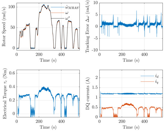
Figure 13.
Experimental results for UDDS speed command with MRASCC FOC.

Table 1.
Performance indices for the IM control schemes evaluated with our experimental EV case study.
Additional details of the results in Figure 13 are shown within the close-up plots in Figure 14 for the 60 to 90 rad/s high-speed range and the 0 to 60 low- to medium-speed range. Both algebraic and MRASCC approaches show similar transient and steady-state behavior. In the medium- and high-speed ranges, both methods present an almost constant speed error of around 1 rad/s. In the low-speed range, both methods present an oscillatory transient speed error under 4 rad/s.
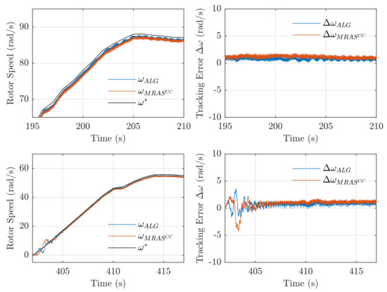
Figure 14.
High- and medium-speed transient zoom for experimental UDDS results with algebraic sensorless and MRASCC FOC.
Further examination of the low-speed range is shown in another close-up shown in Figure 15. Fewer oscillations and speed errors result during the stopping transient, especially for the algebraic approach. The starting transient shows a more challenging condition, but both estimators have errors below 5 rad/s.
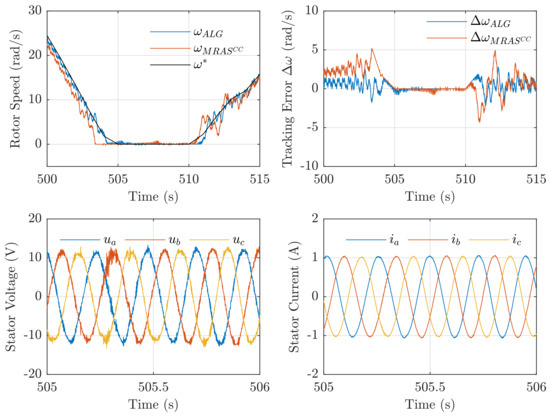
Figure 15.
Low-speed transient zoom for experimental UDDS results with algebraic sensorless and MRASCC FOC including 1s sample of stator voltage and current measurements.
As a last step in the comparison analysis, the experimental stator voltage and current measurements for 1 s in the zero-speed range are also shown in Figure 15. They show some significant noise present in the stator voltage compared to the current measurements. It is also important to highlight that both included an unbalanced DC offset estimated in the range of 100 mV and 10 mA, respectively. Both strategies perform correctly in these experimental voltage and current measurements.
These results suggest that our algebraic estimation strategy is a viable solution for sensorless IM control and our proposed EV case study. On the one hand, the simplicity of the structure associated with the MRASCC alternative compared to our algebraic proposal should not be ignored, as supported by calculations for the computational burden shown in Table A2. On the other hand, emphasis is placed on the facilities to tune and adapt the algebraic estimation strategy. This includes the tuning criteria associated with the sliding-window width T and the availability of a reset scheme to adapt the parameters of the IM model online; see Section 2.2.
5. Discussion
This paper presents an algebraic estimation strategy for sensorless IM control, considering key experimental aspects. We studied its application under the demanding conditions of an EV context, with nominal speed range requirements and highly variant torque loads. Using a laboratory setup for small-scale EV powertrain emulation, we successfully validated its performance with average tracking error rad/s. Its inherent filtering capabilities reached an SNR of 43 dB using our simple single-parameter tuning criteria established in Section 2.1.5. The results further demonstrated coherent performance compared to the well-known MRASCC strategy in [6], without introducing additional dynamics into the control system.
To address some significant challenges of IM speed estimation, we propose a novel estimator design that is different from the classical algebraic methodology. We include the usage of sliding-window integrals from the ideas in [19]. This helps to reduce the distortion introduced by classical filters, a problem described in [13]. Our estimator does not avoid derivative calculations as in [17,19]. Instead, we simplified its structure and used a current derivative estimator described in Section 2.1.3. Unlike sensorless proposals as [13,14], we adapted a resetting scheme from [19] to use pure integrals without floating-point overflow. This scheme potentially facilitates the integration of online parameter adaptation to deal with IM model mismatch effects.
Thus, our work further proves the flexibility and capabilities of the concepts of algebraic methodology to develop new and effective solutions for complex estimation problems. There are still opportunities to expand its numerical analysis, perform parameter sensitivity studies, and improve its computational efficiency. For instance, future work could study our strategy with different control strategies, flux estimators, and parameter adaptation mechanisms. The proposed methods and structures are potentially adaptable to other motor technologies or completely different high-performance applications.
Author Contributions
Conceptualization, J.N.-G., A.B.-P. and J.C.-R.; methodology, J.N.-G., A.B.-P. and J.C.-R.; software, J.N.-G. and A.B.-P.; validation, J.N.-G., A.B.-P. and J.C.-R.; formal analysis, J.N.-G.; investigation, J.N.-G.; resources, J.N.-G. and J.C.-R.; data curation, J.N.-G.; writing—original draft preparation, J.N.-G.; writing—review and editing, J.N.-G., A.B.-P. and J.C.-R.; visualization, J.N.-G.; supervision, A.B.-P. and J.C.-R.; project administration, A.B.-P. and J.C.-R.; funding acquisition, J.C.-R. All authors have read and agreed to the published version of the manuscript.
Funding
This research received no external funding, and the APC was funded by Purdue University Libraries Open Access Publishing Fund.
Data Availability Statement
The raw data supporting the conclusions of this article will be made available by the authors on request.
Conflicts of Interest
The authors declare no conflicts of interest. The funders had no role in the design of the study; in the collection, analyses, or interpretation of data; in the writing of the manuscript; or in the decision to publish the results.
Abbreviations
The following abbreviations are used in this manuscript:
| IM | Induction motor |
| EV | Electric vehicle |
| FOC | Field-oriented control |
| MRAS | Model reference adaptive system |
| UDDS | Urban Dynamometer Driving Schedule |
Appendix A
This section includes experimental values for the IM motor and the EV model. The values result from motor plate information, classical IM parameter identification procedures, and scale-down versions for a real EV.
Table A1.
Parameters for the IM and EV.
Table A1.
Parameters for the IM and EV.
| IM Parameters | Value |
|---|---|
| Rated speed/Pole pairs () | 1500 rpm/2 |
| Rated power/Torque | 100 W/0.6 Nm |
| Rated voltage/Current/Frequency | 70 V/1.2 A/50 Hz |
| Stator ()/Rotor () resistance | 6.576 /19.577 |
| Stator ()/ Rotor () leakage inductance | 55.2 mH/5.4 mH |
| Magnetizing inductance () | 243.4 mH |
| EV parameters (small-scale) | Value |
| Vehicle mass (m)/Frontal Area () | 98 kg/2.4 |
| Wheel radius ()/Fixed gear ratio () | 0.3594 m/9.73 |
| Air density () @ 1 atm, 25 °C | 1.1839 kg/ |
| Aerodynamic drag ()/Rolling resistance () | 0.24/0.002 |
Appendix B
This section includes simulation values using the Simulink Profiler tool. We obtained results for both the algebraic and the MRASCC estimator. Both were tested with the same 109 s simulation speed and torque profiles used for our transient evaluation study. The simulations were executed with the Accelerator mode using an ode4 solver with 0.001 s fixed step. Everything was executed on a laptop with an Intel Core i7-1360H processor, 2.4 GHz base speed, and 10 cores. After five simulations for each estimator, the results show an average for the total execution time of our algebraic estimator block of 0.38 s and 0.0066 s for the MRAS CC estimator block.
Table A2.
Total execution time in seconds for each estimator block using Simulink Profiler.
Table A2.
Total execution time in seconds for each estimator block using Simulink Profiler.
| Simulation | Algebraic Estimator | MRASCC Estimator |
|---|---|---|
| 1 | 0.372412 | 0.006422 |
| 2 | 0.373271 | 0.006539 |
| 3 | 0.372554 | 0.006534 |
| 4 | 0.368123 | 0.006746 |
| 5 | 0.404302 | 0.006769 |
| Mean | 0.38 | 0.0066 |
References
- Hannan, M.; Ali, J.A.; Mohamed, A.; Hussain, A. Optimization techniques to enhance the performance of induction motor drives: A review. Renew. Sustain. Energy Rev. 2018, 81, 1611–1626. [Google Scholar] [CrossRef]
- Dehghan-Azad, E.; Gadoue, S.; Atkinson, D.; Slater, H.; Barrass, P.; Blaabjerg, F. Sensorless Control of IM Based on Stator-Voltage MRAS for Limp-Home EV Applications. IEEE Trans. Power Electron. 2018, 33, 1911–1921. [Google Scholar] [CrossRef]
- Alsofyani, I.M.; Idris, N. A review on sensorless techniques for sustainable reliablity and efficient variable frequency drives of induction motors. Renew. Sustain. Energy Rev. 2013, 24, 111–121. [Google Scholar] [CrossRef]
- Holtz, J. Sensorless Control of Induction Machines With or Without Signal Injection? IEEE Trans. Ind. Electron. 2006, 53, 7–30. [Google Scholar] [CrossRef]
- Kumar, R.; Das, S.; Syam, P.; Chattopadhyay, A.K. Review on model reference adaptive system for sensorless vector control of induction motor drives. IET Electr. Power Appl. 2015, 9, 496–511. [Google Scholar] [CrossRef]
- Orlowska-Kowalska, T.; Dybkowski, M. Stator-Current-Based MRAS Estimator for a Wide Range Speed-Sensorless Induction-Motor Drive. IEEE Trans. Ind. Electron. 2010, 57, 1296–1308. [Google Scholar] [CrossRef]
- Zaky, M.S.; Metwaly, M.K. Sensorless Torque/Speed Control of Induction Motor Drives at Zero and Low Frequencies With Stator and Rotor Resistance Estimations. IEEE J. Emerg. Sel. Top. Power Electron. 2016, 4, 1416–1429. [Google Scholar] [CrossRef]
- Zerdali, E.; Barut, M. The Comparisons of Optimized Extended Kalman Filters for Speed-Sensorless Control of Induction Motors. IEEE Trans. Ind. Electron. 2017, 64, 4340–4351. [Google Scholar] [CrossRef]
- Zhao, L.; Huang, J.; Liu, H.; Li, B.; Kong, W. Second-Order Sliding-Mode Observer with Online Parameter Identification for Sensorless Induction Motor Drives. IEEE Trans. Ind. Electron. 2014, 61, 5280–5289. [Google Scholar] [CrossRef]
- Harnefors, L.; Hinkkanen, M. Stabilization Methods for Sensorless Induction Motor Drives A Survey. IEEE J. Emerg. Sel. Top. Power Electron. 2014, 2, 132–142. [Google Scholar] [CrossRef]
- Zhang, Y.; Zhao, Z.; Lu, T.; Yuan, L.; Xu, W.; Zhu, J. A comparative study of Luenberger observer, sliding mode observer and extended Kalman filter for sensorless vector control of induction motor drives. In Proceedings of the 2009 IEEE Energy Conversion Congress and Exposition, San Jose, CA, USA, 20–24 September 2009; pp. 2466–2473. [Google Scholar] [CrossRef]
- Maiti, S.; Verma, V.; Chakraborty, C.; Hori, Y. An Adaptive Speed Sensorless Induction Motor Drive With Artificial Neural Network for Stability Enhancement. IEEE Trans. Ind. Inform. 2012, 8, 757–766. [Google Scholar] [CrossRef]
- Stojić, D.; Milinković, M.; Veinović, S.; Klasnić, I. Improved Stator Flux Estimator for Speed Sensorless Induction Motor Drives. IEEE Trans. Power Electron. 2015, 30, 2363–2371. [Google Scholar] [CrossRef]
- Holtz, J.; Quan, J. Sensorless vector control of induction motors at very low speed using a nonlinear inverter model and parameter identification. IEEE Trans. Ind. Appl. 2002, 38, 1087–1095. [Google Scholar] [CrossRef]
- Fliess, M.; Sira-Ramírez, H. An algebraic framework for linear identification. ESAIM COCV 2003, 9, 151–168. [Google Scholar] [CrossRef]
- Fliess, M.; Join, C.; Sira-Ramirez, H. Non-linear estimation is easy. Int. J. Model. Identif. Control 2008, 4, 12–27. [Google Scholar] [CrossRef]
- Sira-Ramírez, H.; García-Rodríguez, C.; Cortés-Romero, J.; Luviano-Juárez, A. Algebraic Identification and Estimation Methods in Feedback Control Systems; John Wiley & Sons, Ltd.: Chichester, UK, 2014. [Google Scholar]
- Cortés-Romero, J.; García-Rodríguez, C.; Luviano-Juárez, A.; Sira-Ramírez, H.; Garcia-Rodriguez, C.; Luviano-Juarez, A.; Sira-Ramírez, H. Algebraic parameter identification for induction motors. In Proceedings of the IECON 2011—37th Annual Conference of the IEEE Industrial Electronics Society, Melbourne, Australia, 7–10 November 2011; pp. 1734–1740. [Google Scholar] [CrossRef]
- Cortés-Romero, J.; Jimenez-Triana, A.; Coral-Enriquez, H.; Sira-Ramírez, H. Algebraic estimation and active disturbance rejection in the control of flat systems. Control Eng. Pract. 2017, 61, 173–182. [Google Scholar] [CrossRef]
- Chiasson, J. Modeling and High-Performance Control of Electric Machines; John Wiley & Sons, Inc.: Hoboken, NJ, USA, 2005. [Google Scholar] [CrossRef]
- Trefethen, L. Numerical Linear Algebra; Society for Industrial and Applied Mathematics: Philadelphia, PA, USA, 1997. [Google Scholar]
- Canudas De Wit, C.; Youssef, A.; Barbot, J.; Martin, P.; Malrait, F. Observability conditions of induction motors at low frequencies. In Proceedings of the 39th IEEE Conference on Decision and Control, Sydney, Australia, 12–15 December 2000; Volume 3, pp. 2044–2049. [Google Scholar] [CrossRef]
- Park, G.; Lee, S.; Jin, S.; Kwak, S. Integrated modeling and analysis of dynamics for electric vehicle powertrains. Expert Syst. Appl. 2014, 41, 2595–2607. [Google Scholar] [CrossRef]
- Haddoun, A.; Benbouzid, M.E.H.; Diallo, D.; Abdessemed, R.; Ghouili, J.; Srairi, K. A Loss-Minimization DTC Scheme for EV Induction Motors. IEEE Trans. Veh. Technol. 2007, 56, 81–88. [Google Scholar] [CrossRef]
Disclaimer/Publisher’s Note: The statements, opinions and data contained in all publications are solely those of the individual author(s) and contributor(s) and not of MDPI and/or the editor(s). MDPI and/or the editor(s) disclaim responsibility for any injury to people or property resulting from any ideas, methods, instructions or products referred to in the content. |
© 2024 by the authors. Licensee MDPI, Basel, Switzerland. This article is an open access article distributed under the terms and conditions of the Creative Commons Attribution (CC BY) license (https://creativecommons.org/licenses/by/4.0/).