
Deep Clustering by Graph Attention Contrastive Learning


Abstract
1. Introduction
- We propose a novel graph attention contrastive learning framework. By selecting and filtering samples through our graph attention framework, we can introduce more confident and informative semantic pairs to the clustering task and thus further improve clustering performance.
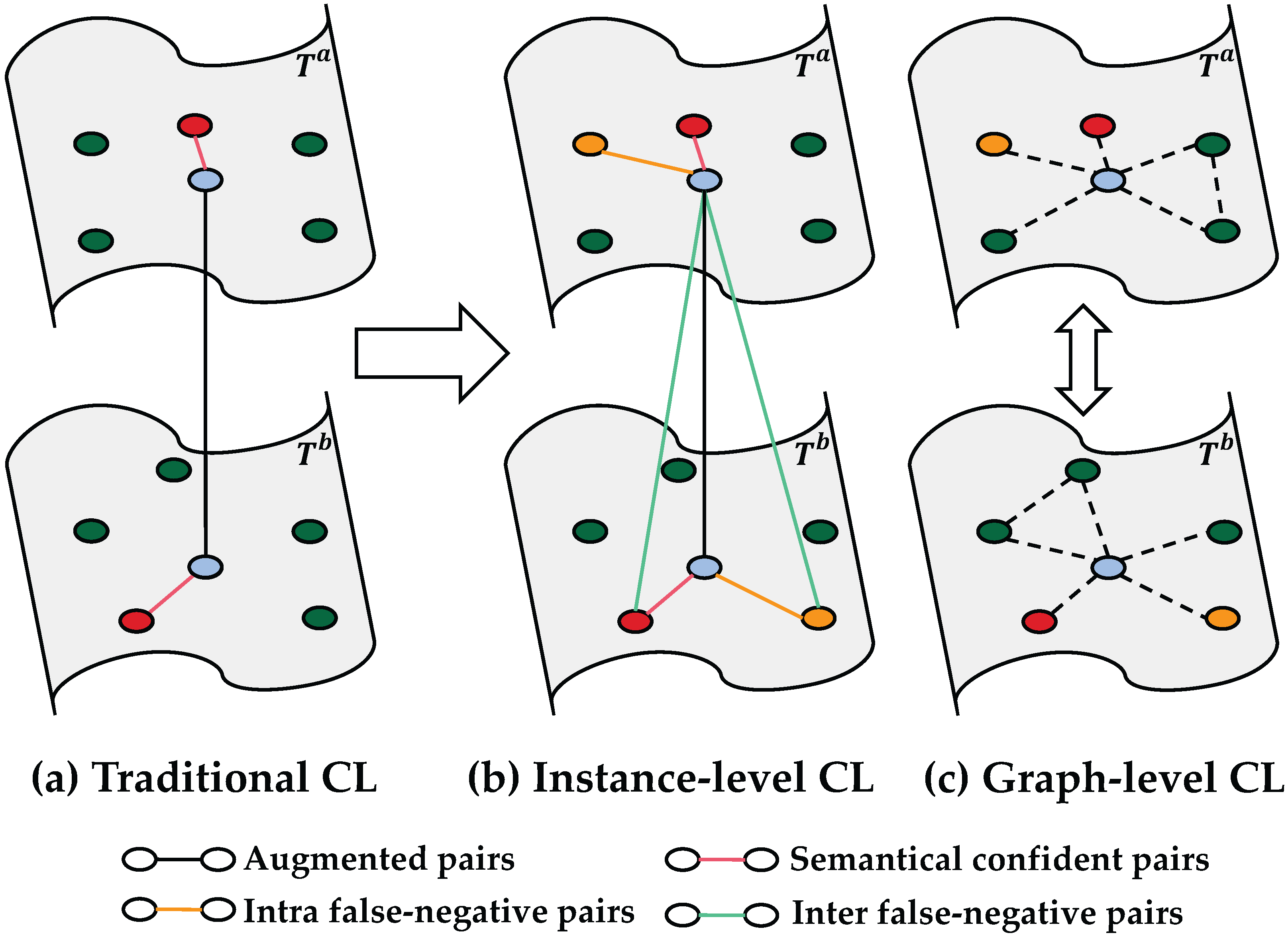
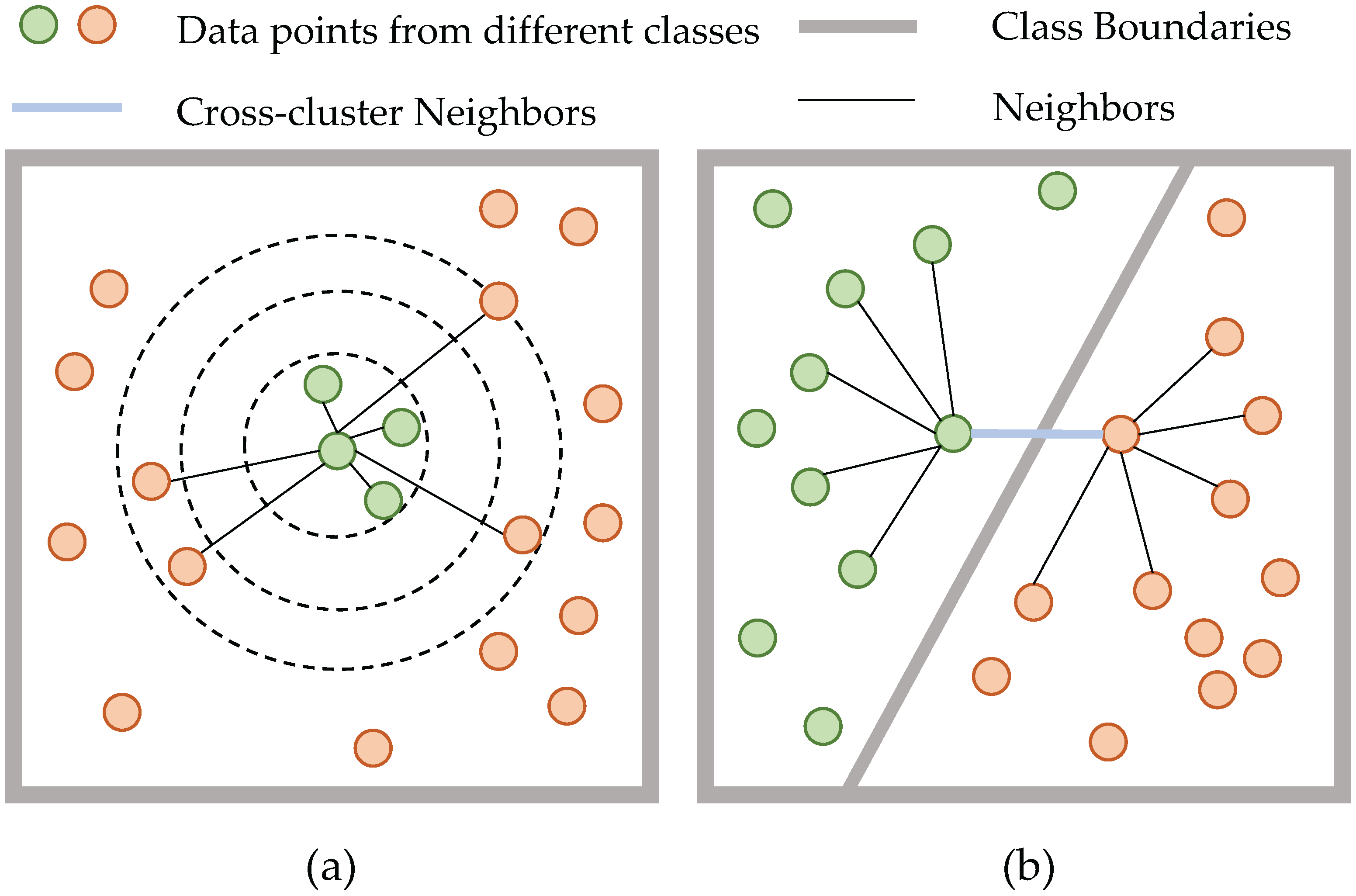
- Instance-level contrastive learning treats the local false-negative pairs as positive pairs, including the inter-graph and intra-graph situations. Meanwhile, the graph-level contrastive learning constrains neighbors’ relationships from a global perspective.
- We conduct extensive experiments on the image clustering task, and our proposed method achieves significant improvements on various datasets. We also conduct extensive ablation and case studies to validate the effectiveness of each proposed module.
2. Related Work
2.1. Deep Clustering
2.2. Graph-Based Clustering
2.3. Deep Contrastive Clustering
3. Method
3.1. Preliminaries
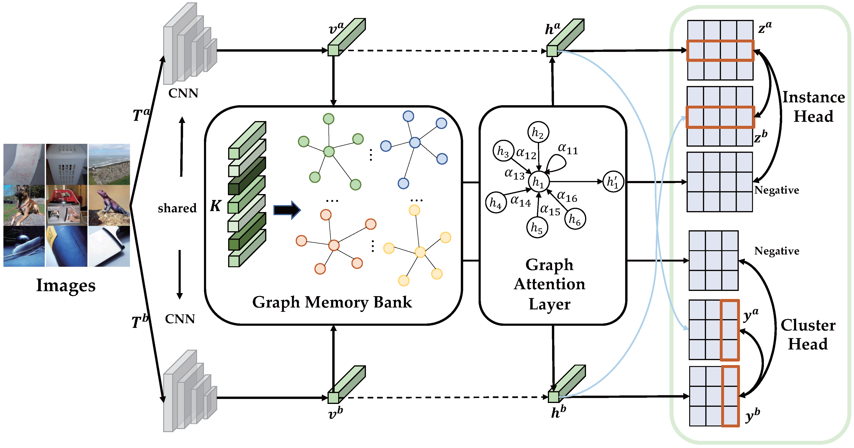
3.2. Framework
3.2.1. Graph Construction Layer
3.2.2. Graph Attention Layer
3.2.3. Instance-Level Contrastive Learning
3.2.4. Graph-Level Contrastive Learning
3.3. Model Training
| Algorithm 1:Graph Attention Contrastive Learning. |
|
4. Experiments
4.1. Datasets
- CIFAR-10/100: [43] A commonly used dataset with a joint set of 50,000 training images and 10,000 testing images for clustering. In CIFAR-100, the 20 super-classes are considered ground-truth labels. The image size is fixed to .
- STL-10: [44] An image recognition dataset consisting of 500/800 training/test images for each of 10 classes. An additional 100,000 samples from several unknown classes are also used for the training stage. The image size is fixed to .
- ImageNet-10 and ImageNet-Dogs: [40] The ImageNet subsets contain samples from 10 randomly selected classes or 15 dog breeds with each class composed of 1300 images. The image size is fixed to .
- Tiny-ImageNet: [45] Another ImageNet subset on a larger scale, with samples evenly distributed in 200 classes. The image size is fixed to .
4.2. Evaluation Metrics
4.3. Experimental Settings
4.4. Performance Comparison
4.5. Ablation Study
4.5.1. Effect of the Proposed Losses
4.5.2. Effect of the Number of Nearest Neighbors
4.6. Qualitative Study
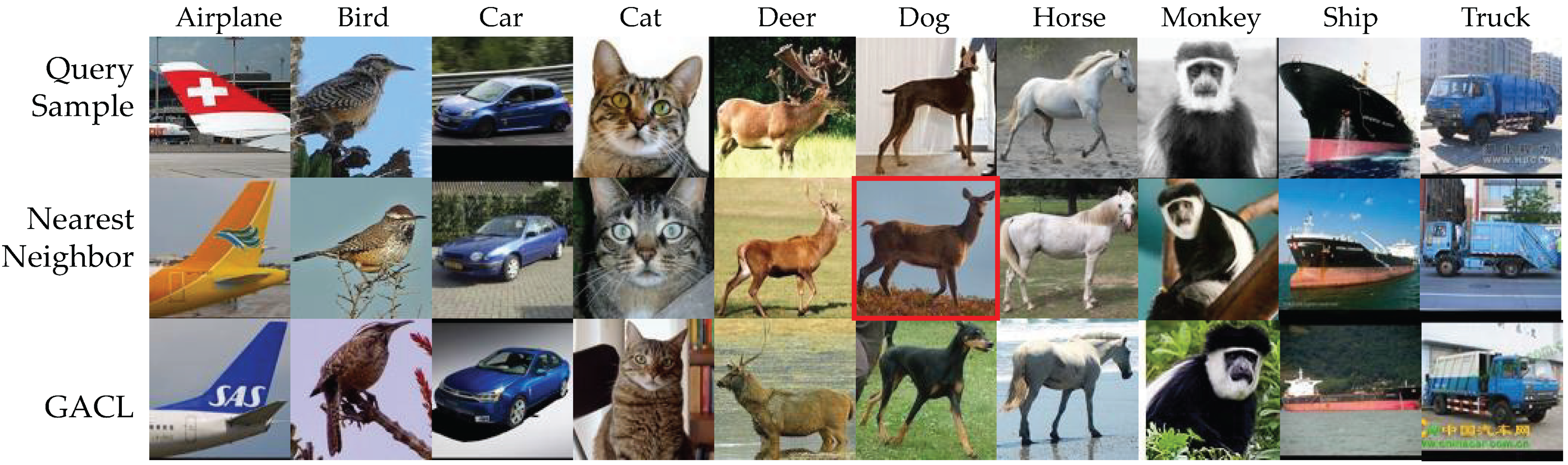
4.6.1. Visualization on the Most Confident Neighbors
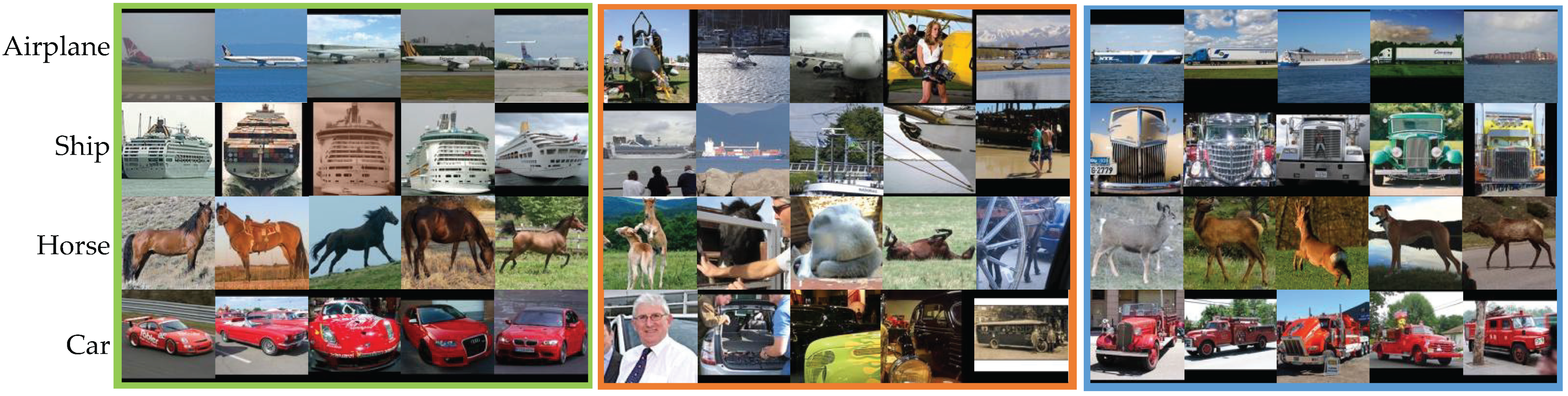
4.6.2. Visualization on Classification Results
5. Conclusions
Author Contributions
Funding
Institutional Review Board Statement
Informed Consent Statement
Data Availability Statement
Conflicts of Interest
References
- Xie, Y.; Chen, T.; Pu, T.; Wu, H.; Lin, L. Adversarial Graph Representation Adaptation for Cross-Domain Facial Expression Recognition. In Proceedings of the The 28th ACM International Conference on Multimedia, Virtual Event/Seattle, WA, USA, 12–16 October 2020; Chen, C.W., Cucchiara, R., Hua, X., Qi, G., Ricci, E., Zhang, Z., Zimmermann, R., Eds.; ACM International: New York, NY, USA, 2020; pp. 1255–1264. [Google Scholar]
- Luo, Y.; Huang, Z.; Wang, Z.; Zhang, Z.; Baktashmotlagh, M. Adversarial Bipartite Graph Learning for Video Domain Adaptation. In Proceedings of the The 28th ACM International Conference on Multimedia, Virtual Event/Seattle, WA, USA, 12–16 October 2020; Chen, C.W., Cucchiara, R., Hua, X., Qi, G., Ricci, E., Zhang, Z., Zimmermann, R., Eds.; ACM International: New York, NY, USA, 2020; pp. 19–27. [Google Scholar]
- Wang, C.; Li, L.; Zhang, H.; Li, D. Quaternion-based knowledge graph neural network for social recommendation. Knowl. Based Syst. 2022, 257, 109940. [Google Scholar] [CrossRef]
- Thota, M.; Leontidis, G. Contrastive Domain Adaptation. In Proceedings of the IEEE Conference on Computer Vision and Pattern Recognition Workshops, CVPR Workshops 2021, Virtual, 19–25 June 2021; Computer Vision Foundation/IEEE: Nashville, TN, USA, 2021; pp. 2209–2218. [Google Scholar]
- Kang, G.; Jiang, L.; Yang, Y.; Hauptmann, A.G. Contrastive Adaptation Network for Unsupervised Domain Adaptation. In Proceedings of the IEEE Conference on Computer Vision and Pattern Recognition, CVPR 2019, Long Beach, CA, USA, 16–20 June 2019; Computer Vision Foundation/IEEE: Long Beach, CA, USA, 2019; pp. 4893–4902. [Google Scholar]
- Mekhazni, D.; Dufau, M.; Desrosiers, C.; Pedersoli, M.; Granger, E. Camera Alignment and Weighted Contrastive Learning for Domain Adaptation in Video Person ReID. In Proceedings of the IEEE/CVF Winter Conference on Applications of Computer Vision, WACV 2023, Waikoloa, HI, USA, 2–7 January 2023; pp. 1624–1633. [Google Scholar]
- MacQueen, J. Some methods for classification and analysis of multivariate observations. In Fifth Berkeley Symposium on Mathematical Statistics and Probability; University of California: Los Angeles, CA, USA, 1967; pp. 281–297. [Google Scholar]
- Shi, J.; Malik, J. Normalized Cuts and Image Segmentation. IEEE Trans. Pattern Anal. Mach. Intell. 2000, 22, 888–905. [Google Scholar]
- Li, X.; Zhang, R.; Wang, Q.; Zhang, H. Autoencoder Constrained Clustering With Adaptive Neighbors. IEEE Trans. Neural Netw. Learn. Syst. 2020, 32, 443–449. [Google Scholar] [CrossRef] [PubMed]
- Xie, J.; Girshick, R.B.; Farhadi, A. Unsupervised Deep Embedding for Clustering Analysis. In Proceedings of the 2016 International Conference on Machine Learning, New York, NY, USA, 19–24 June 2016; pp. 478–487. [Google Scholar]
- Yang, J.; Parikh, D.; Batra, D. Joint Unsupervised Learning of Deep Representations and Image Clusters. In Proceedings of the 2016 Conference on Computer Vision and Pattern Recognition, Las Vegas, NV, USA, 26 June–1 July 2016; pp. 5147–5156. [Google Scholar]
- Caron, M.; Bojanowski, P.; Joulin, A.; Douze, M. Deep Clustering for Unsupervised Learning of Visual Features. In Proceedings of the 15th European Conference on Computer Vision, 8–14 September 2018; Ferrari, V., Hebert, M., Sminchisescu, C., Weiss, Y., Eds.; Springer: Munich, Germany, 2018; pp. 139–156. [Google Scholar]
- He, K.; Fan, H.; Wu, Y.; Xie, S.; Girshick, R. Momentum contrast for unsupervised visual representation learning. In Proceedings of the 2020 Conference on Computer Vision and Pattern Recognition, Seattle, WA, USA, 14–19 June 2020; pp. 9729–9738. [Google Scholar]
- Chen, T.; Kornblith, S.; Norouzi, M.; Hinton, G.E. A Simple Framework for Contrastive Learning of Visual Representations. In Proceedings of the 2020 International Conference on Machine Learning, Virtual, 12–18 July 2020; pp. 1597–1607. [Google Scholar]
- Li, Y.; Hu, P.; Liu, J.Z.; Peng, D.; Zhou, J.T.; Peng, X. Contrastive Clustering. In Proceedings of the 2021 AAAI Conference on Artificial Intelligence, Virtually, 2–9 February 2021; pp. 8547–8555. [Google Scholar]
- Ji, X.; Vedaldi, A.; Henriques, J.F. Invariant Information Clustering for Unsupervised Image Classification and Segmentation. In Proceedings of the 2019 International Conference on Computer Vision, Seoul, Republic of Korea, 27 October–2 November 2019; pp. 9864–9873. [Google Scholar]
- Wu, J.; Long, K.; Wang, F.; Qian, C.; Li, C.; Lin, Z.; Zha, H. Deep Comprehensive Correlation Mining for Image Clustering. In Proceedings of the 2019 International Conference on Computer Vision, Seoul, Republic of Korea, 27 October–2 November 2019; pp. 8149–8158. [Google Scholar]
- Dang, Z.; Deng, C.; Yang, X.; Wei, K.; Huang, H. Nearest Neighbor Matching for Deep Clustering. In Proceedings of the IEEE Conference on Computer Vision and Pattern Recognition Workshops, CVPR Workshops 2021, Virtual, 19–25 June 2021; pp. 13693–13702. [Google Scholar]
- Van Gansbeke, W.; Vandenhende, S.; Georgoulis, S.; Proesmans, M.; Van Gool, L. Scan: Learning to classify images without labels. In Proceedings of the 2020 European Conference on Computer Vision, Glasgow, UK, 23–28 August 2020; pp. 268–285. [Google Scholar]
- Yang, B.; Fu, X.; Sidiropoulos, N.D.; Hong, M. Towards K-means-friendly Spaces: Simultaneous Deep Learning and Clustering. In Proceedings of the 2017 International Conference on Machine Learning, Sydney, Australia, 6–11 August 2017; pp. 3861–3870. [Google Scholar]
- Wang, C.; Pan, S.; Hu, R.; Long, G.; Jiang, J.; Zhang, C. Attributed Graph Clustering: A Deep Attentional Embedding Approach. In Proceedings of the Twenty-Eighth International Joint Conference on Artificial Intelligence, IJCAI 2019, Macao, China, 10–16 August 2019; Kraus, S., Ed.; Elsevier: Macao, China, 2019; pp. 3670–3676. [Google Scholar]
- Bo, D.; Wang, X.; Shi, C.; Zhu, M.; Lu, E.; Cui, P. Structural Deep Clustering Network. In Proceedings of the WWW ’20: The Web Conference 2020, Taipei, Taiwan, 20–24 April 2020; Huang, Y., King, I., Liu, T., van Steen, M., Eds.; ACM: Taipei, Taiwan, 2020; pp. 1400–1410. [Google Scholar]
- Tu, W.; Zhou, S.; Liu, X.; Guo, X.; Cai, Z.; Zhu, E.; Cheng, J. Deep Fusion Clustering Network. In Proceedings of the Thirty-Fifth AAAI Conference on Artificial Intelligence the Thirty-Third Conference on Innovative Applications of Artificial Intelligence The Eleventh Symposium on Educational Advances in Artificial Intelligence Sponsored by the Association for the Advancement of Artificial Intelligence, Virtually, 2–9 February 2021; AAAI: New York, NY, USA, 2021; pp. 9978–9987. [Google Scholar]
- Peng, Z.; Liu, H.; Jia, Y.; Hou, J. Attention-driven Graph Clustering Network. In Proceedings of the MM ’21: ACM Multimedia Conference, Virtual Event, China, 20–24 October 2021; Shen, H.T., Zhuang, Y., Smith, J.R., Yang, Y., César, P., Metze, F., Prabhakaran, B., Eds.; ACM: New York, NY, USA, 2021; pp. 935–943. [Google Scholar]
- Pan, S.; Hu, R.; Fung, S.; Long, G.; Jiang, J.; Zhang, C. Learning Graph Embedding With Adversarial Training Methods. IEEE Trans. Cybern. 2020, 50, 2475–2487. [Google Scholar] [CrossRef] [PubMed]
- Pan, S.; Hu, R.; Long, G.; Jiang, J.; Yao, L.; Zhang, C. Adversarially Regularized Graph Autoencoder for Graph Embedding. In Proceedings of the Twenty-Seventh International Joint Conference on Artificial Intelligence, IJCAI 2018, Stockholm, Sweden, 13–19 July 2018; Lang, J., Ed.; Elsevier: Stockholm, Sweden, 2018; pp. 2609–2615. [Google Scholar]
- Tao, Z.; Liu, H.; Li, J.; Wang, Z.; Fu, Y. Adversarial Graph Embedding for Ensemble Clustering. In Proceedings of the Twenty-Eighth International Joint Conference on Artificial Intelligence, IJCAI 2019, Macao, China, 10–16 August 2019; Kraus, S., Ed.; Elsevier: Macao, China, 2019; pp. 3562–3568. [Google Scholar]
- Cui, G.; Zhou, J.; Yang, C.; Liu, Z. Adaptive Graph Encoder for Attributed Graph Embedding. In Proceedings of the KDD ’20: The 26th ACM SIGKDD Conference on Knowledge Discovery and Data Mining, Virtual Event, CA, USA, 23–27 August 2020; Gupta, R., Liu, Y., Tang, J., Prakash, B.A., Eds.; ACM: New York, NY, USA, 2020; pp. 976–985. [Google Scholar]
- Liu, L.; Kang, Z.; Ruan, J.; He, X. Multilayer graph contrastive clustering network. Inf. Sci. 2022, 613, 256–267. [Google Scholar] [CrossRef]
- Xia, W.; Gao, Q.; Yang, M.; Gao, X. Self-supervised Contrastive Attributed Graph Clustering. arXiv 2021, arXiv:2110.08264. [Google Scholar]
- Wang, C.; Pan, S.; Long, G.; Zhu, X.; Jiang, J. MGAE: Marginalized Graph Autoencoder for Graph Clustering. In Proceedings of the 2017 ACM on Conference on Information and Knowledge Management, CIKM 2017, Singapore, 6–10 November 2017; Lim, E., Winslett, M., Sanderson, M., Fu, A.W., Sun, J., Culpepper, J.S., Lo, E., Ho, J.C., Donato, D., Agrawal, R., et al., Eds.; ACM: New York, NY, USA, 2017; pp. 889–898. [Google Scholar]
- Kipf, T.N.; Welling, M. Variational Graph Auto-Encoders. arXiv 2016, arXiv:1611.07308. [Google Scholar]
- Cheng, J.; Wang, Q.; Tao, Z.; Xie, D.; Gao, Q. Multi-View Attribute Graph Convolution Networks for Clustering. In Proceedings of the Twenty-Ninth International Joint Conference on Artificial Intelligence, IJCAI, Yokohama, Japan, 11–17 July 2020; Bessiere, C., Ed.; Elsevier: Yokohama, Japan, 2020; pp. 2973–2979. [Google Scholar]
- Vaswani, A.; Shazeer, N.; Parmar, N.; Uszkoreit, J.; Jones, L.; Gomez, A.N.; Kaiser, L.; Polosukhin, I. Attention is All you Need. In Proceedings of the Advances in Neural Information Processing Systems 30: Annual Conference on Neural Information Processing Systems 2017, Long Beach, CA, USA, 4–9 December 2017; Guyon, I., von Luxburg, U., Bengio, S., Wallach, H.M., Fergus, R., Vishwanathan, S.V.N., Garnett, R., Eds.; MIT: Long Beach, CA, USA, 2017; pp. 5998–6008. [Google Scholar]
- Park, J.; Lee, M.; Chang, H.J.; Lee, K.; Choi, J.Y. Symmetric Graph Convolutional Autoencoder for Unsupervised Graph Representation Learning. In Proceedings of the 2019 International Conference on Computer Vision, Seoul, Republic of Korea, 27 October–2 November 2019; pp. 6518–6527. [Google Scholar]
- Zhang, X.; Liu, H.; Li, Q.; Wu, X. Attributed Graph Clustering via Adaptive Graph Convolution. In Proceedings of the Twenty-Eighth International Joint Conference on Artificial Intelligence, IJCAI 2019, Macao, China, 10–16 August 2019; Kraus, S., Ed.; Elsevier: Macao, China, 2019; pp. 4327–4333. [Google Scholar]
- Hadsell, R.; Chopra, S.; LeCun, Y. Dimensionality Reduction by Learning an Invariant Mapping. In Proceedings of the EEE Computer Society Conference on Computer Vision and Pattern Recognition, New York, NY, USA, 17–22 June 2006; pp. 1735–1742. [Google Scholar]
- Sharma, V.; Tapaswi, M.; Sarfraz, M.S.; Stiefelhagen, R. Clustering based Contrastive Learning for Improving Face Representations. In Proceedings of the 2020 15th IEEE International Conference on Automatic Face and Gesture Recognition (FG 2020), Buenos Aires, Argentina, 16–20 November 2020; pp. 109–116. [Google Scholar]
- Dosovitskiy, A.; Springenberg, J.T.; Riedmiller, M.A.; Brox, T. Discriminative Unsupervised Feature Learning with Convolutional Neural Networks. In Proceedings of the Annual Conference on Neural Information Processing Systems 2014, Montreal, QC, Canada, 8–13 December 2014; pp. 766–774. [Google Scholar]
- Chang, J.; Wang, L.; Meng, G.; Xiang, S.; Pan, C. Deep Adaptive Image Clustering. In Proceedings of the International Conference on Computer Vision, Venice, Italy, 17–31 July 2017; pp. 5880–5888. [Google Scholar]
- Schroff, F.; Kalenichenko, D.; Philbin, J. FaceNet: A unified embedding for face recognition and clustering. In Proceedings of the IEEE Conference on Computer Vision and Pattern Recognition (CVPR), Boston, MA, USA, 7–12 June 2015; pp. 815–823. [Google Scholar]
- Huang, J.; Gong, S.; Zhu, X. Deep Semantic Clustering by Partition Confidence Maximisation. In Proceedings of the IEEE Conference on Computer Vision and Pattern Recognition, Boston, MA, USA, 7–12 June 2020; pp. 8846–8855. [Google Scholar]
- Krizhevsky, A.; Hinton, G. Learning Multiple Layers of Features from Tiny Images. 2009. Available online: http://www.cs.utoronto.ca/~kriz/learning-features-2009-TR.pdf (accessed on 8 April 2009).
- Coates, A.; Ng, A.Y.; Lee, H. An Analysis of Single-Layer Networks in Unsupervised Feature Learning. In Proceedings of the International Conference on Artificial Intelligence and Statistics, Fort Lauderdale, FL, USA, 11–13 April 2011; Gordon, G.J., Dunson, D.B., Dudík, M., Eds.; AISTATS: Fort Laud- erdale, FL, USA, 2011; pp. 215–223. [Google Scholar]
- Le, Y.; Yang, X. Tiny imagenet visual recognition challenge. CS 231N 2015, 7, 3. [Google Scholar]
- Gowda, K.C.; Krishna, G. Agglomerative clustering using the concept of mutual nearest neighbourhood. Pattern Recognit. 1978, 10, 105–112. [Google Scholar] [CrossRef]
- Cai, D.; He, X.; Wang, X.; Bao, H.; Han, J. Locality Preserving Nonnegative Matrix Factorization. In Proceedings of the International Joint Conference on Artificial Intelligence, Pasadena, CA, USA, 11–17 July 2009; Boutilier, C., Ed.; Elsevier: Pasadena, CA, USA, 2009; pp. 1010–1015. [Google Scholar]
- Bengio, Y.; Lamblin, P.; Popovici, D.; Larochelle, H. Greedy Layer-Wise Training of Deep Networks. In Proceedings of the Annual Conference on Neural Information Processing Systems, Vancouver, BC, Canada, 4–7 December 2006; Schölkopf, B., Platt, J.C., Hofmann, T., Eds.; MIT: Vancouver, BC, Canada, 2006; pp. 153–160. [Google Scholar]
- Radford, A.; Metz, L.; Chintala, S. Unsupervised Representation Learning with Deep Convolutional Generative Adversarial Networks. In Proceedings of the International Conference on Learning Representations, San Juan, Puerto Rico, 2–4 May 2016. [Google Scholar]
- Zeiler, M.D.; Krishnan, D.; Taylor, G.W.; Fergus, R. Deconvolutional networks. In Proceedings of the 2020 Conference on Computer Vision and Pattern Recognition, Seattle, WA, USA, 14–19 June 2020; pp. 2528–2535. [Google Scholar]
- Kingma, D.P.; Welling, M. Auto-Encoding Variational Bayes. In Proceedings of the International Conference on Learning Representations, Banff, AB, Canada, 14–16 April 2014. [Google Scholar]
- Dang, Z.; Deng, C.; Yang, X.; Huang, H. Doubly Contrastive Deep Clustering. arXiv 2021, arXiv:2103.05484. [Google Scholar]
- Zhong, H.; Wu, J.; Chen, C.; Huang, J.; Deng, M.; Nie, L.; Lin, Z.; Hua, X. Graph Contrastive Clustering. arXiv 2021, arXiv:2104.01429. [Google Scholar]


| Datasets Metrics | CIFAR-10 | CIFAR-100 | STL-10 | ImageNet-10 | ImageNet-Dogs | Tiny-ImageNet | ||||||||||||
|---|---|---|---|---|---|---|---|---|---|---|---|---|---|---|---|---|---|---|
| NMI | ACC | ARI | NMI | ACC | ARI | NMI | ACC | ARI | NMI | ACC | ARI | NMI | ACC | ARI | NMI | ACC | ARI | |
| K-means | 0.087 | 0.229 | 0.049 | 0.084 | 0.130 | 0.028 | 0.125 | 0.192 | 0.061 | 0.119 | 0.241 | 0.057 | 0.055 | 0.105 | 0.020 | 0.065 | 0.025 | 0.005 |
| SC | 0.103 | 0.247 | 0.085 | 0.090 | 0.136 | 0.022 | 0.098 | 0.159 | 0.048 | 0.151 | 0.274 | 0.076 | 0.038 | 0.111 | 0.013 | 0.063 | 0.022 | 0.004 |
| AC | 0.105 | 0.228 | 0.065 | 0.098 | 0.138 | 0.034 | 0.239 | 0.332 | 0.140 | 0.138 | 0.242 | 0.067 | 0.037 | 0.139 | 0.021 | 0.069 | 0.027 | 0.005 |
| NMF | 0.081 | 0.190 | 0.034 | 0.079 | 0.118 | 0.026 | 0.096 | 0.180 | 0.046 | 0.132 | 0.230 | 0.065 | 0.044 | 0.118 | 0.016 | 0.072 | 0.029 | 0.005 |
| AE | 0.239 | 0.314 | 0.169 | 0.100 | 0.165 | 0.048 | 0.250 | 0.303 | 0.161 | 0.210 | 0.317 | 0.152 | 0.104 | 0.185 | 0.073 | 0.131 | 0.041 | 0.007 |
| DAE | 0.251 | 0.297 | 0.163 | 0.111 | 0.151 | 0.046 | 0.224 | 0.302 | 0.152 | 0.206 | 0.304 | 0.138 | 0.104 | 0.190 | 0.078 | 0.127 | 0.039 | 0.007 |
| DCGAN | 0.265 | 0.315 | 0.176 | 0.120 | 0.151 | 0.045 | 0.210 | 0.298 | 0.139 | 0.225 | 0.346 | 0.157 | 0.121 | 0.174 | 0.078 | 0.135 | 0.041 | 0.007 |
| DeCNN | 0.240 | 0.282 | 0.174 | 0.092 | 0.133 | 0.038 | 0.227 | 0.299 | 0.162 | 0.186 | 0.313 | 0.142 | 0.098 | 0.175 | 0.073 | 0.111 | 0.035 | 0.006 |
| VAE | 0.245 | 0.291 | 0.167 | 0.108 | 0.152 | 0.040 | 0.200 | 0.282 | 0.146 | 0.193 | 0.334 | 0.168 | 0.107 | 0.179 | 0.079 | 0.113 | 0.036 | 0.006 |
| JULE | 0.192 | 0.272 | 0.138 | 0.103 | 0.137 | 0.033 | 0.182 | 0.277 | 0.164 | 0.175 | 0.300 | 0.138 | 0.054 | 0.138 | 0.028 | 0.102 | 0.033 | 0.006 |
| DEC | 0.257 | 0.301 | 0.161 | 0.136 | 0.185 | 0.050 | 0.276 | 0.359 | 0.186 | 0.282 | 0.381 | 0.203 | 0.122 | 0.195 | 0.079 | 0.115 | 0.037 | 0.007 |
| DAC | 0.396 | 0.522 | 0.306 | 0.185 | 0.238 | 0.088 | 0.366 | 0.470 | 0.257 | 0.394 | 0.527 | 0.302 | 0.219 | 0.275 | 0.111 | 0.190 | 0.066 | 0.017 |
| ADC | - | 0.325 | - | - | 0.160 | - | - | 0.530 | - | - | - | - | - | - | - | - | - | - |
| DDC | 0.424 | 0.524 | 0.329 | - | - | - | 0.371 | 0.489 | 0.267 | 0.433 | 0.577 | 0.345 | - | - | - | - | - | - |
| DCCM | 0.496 | 0.623 | 0.408 | 0.285 | 0.327 | 0.173 | 0.376 | 0.482 | 0.262 | 0.608 | 0.710 | 0.555 | 0.321 | 0.383 | 0.182 | 0.224 | 0.108 | 0.038 |
| IIC | - | 0.617 | - | - | 0.257 | - | - | 0.610 | - | - | - | - | - | - | - | - | - | - |
| PICA | 0.591 | 0.696 | 0.512 | 0.310 | 0.337 | 0.171 | 0.611 | 0.713 | 0.531 | 0.802 | 0.870 | 0.761 | 0.352 | 0.352 | 0.201 | 0.277 | 0.098 | 0.040 |
| DCDC | 0.585 | 0.699 | 0.506 | 0.310 | 0.349 | 0.179 | 0.621 | 0.734 | 0.547 | 0.817 | 0.879 | 0.787 | 0.360 | 0.365 | 0.207 | 0.287 | 0.103 | 0.047 |
| CC | 0.705 | 0.790 | 0.637 | 0.431 | 0.429 | 0.266 | 0.764 | 0.850 | 0.726 | 0.859 | 0.893 | 0.822 | 0.445 | 0.429 | 0.274 | 0.340 | 0.140 | 0.071 |
| GCC | 0.764 | 0.856 | 0.728 | 0.472 | 0.472 | 0.305 | 0.684 | 0.788 | 0.631 | 0.842 | 0.901 | 0.822 | 0.490 | 0.526 | 0.362 | 0.347 | 0.138 | 0.075 |
| NNM | 0.748 | 0.843 | 0.709 | 0.484 | 0.477 | 0.316 | 0.694 | 0.808 | 0.650 | 0.867 | 0.913 | 0.844 | 0.497 | 0.533 | 0.373 | 0.356 | 0.144 | 0.081 |
| GACL | 0.793 | 0.875 | 0.753 | 0.496 | 0.488 | 0.321 | 0.783 | 0.863 | 0.744 | 0.871 | 0.903 | 0.841 | 0.513 | 0.543 | 0.397 | 0.356 | 0.148 | 0.079 |
| GACL | w/o | w/o | w/o | w/o | w/o | w/o | |
|---|---|---|---|---|---|---|---|
| NMI | 0.793 | 0.703 | 0.764 | 0.314 | 0.734 | 0.751 | 0.750 |
| ACC | 0.875 | 0.807 | 0.845 | 0.462 | 0.826 | 0.835 | 0.834 |
| ARI | 0.753 | 0.691 | 0.726 | 0.338 | 0.718 | 0.717 | 0.721 |
| K-Nearest Neighbor | 1 | 3 | 5 | 8 | 12 |
|---|---|---|---|---|---|
| NMI | 0.728 | 0.762 | 0.793 | 0.791 | 0.795 |
| ACC | 0.815 | 0.849 | 0.875 | 0.872 | 0.878 |
| ARI | 0.703 | 0.722 | 0.753 | 0.749 | 0.755 |
Disclaimer/Publisher’s Note: The statements, opinions and data contained in all publications are solely those of the individual author(s) and contributor(s) and not of MDPI and/or the editor(s). MDPI and/or the editor(s) disclaim responsibility for any injury to people or property resulting from any ideas, methods, instructions or products referred to in the content. |
© 2023 by the authors. Licensee MDPI, Basel, Switzerland. This article is an open access article distributed under the terms and conditions of the Creative Commons Attribution (CC BY) license (https://creativecommons.org/licenses/by/4.0/).
Share and Cite
Liu, M.; Liu, C.; Fu, X.; Wang, J.; Li, J.; Qi, Q.; Liao, J. Deep Clustering by Graph Attention Contrastive Learning. Electronics 2023, 12, 2489. https://doi.org/10.3390/electronics12112489
Liu M, Liu C, Fu X, Wang J, Li J, Qi Q, Liao J. Deep Clustering by Graph Attention Contrastive Learning. Electronics. 2023; 12(11):2489. https://doi.org/10.3390/electronics12112489
Chicago/Turabian StyleLiu, Ming, Cong Liu, Xiaoyuan Fu, Jing Wang, Jiankun Li, Qi Qi, and Jianxin Liao. 2023. "Deep Clustering by Graph Attention Contrastive Learning" Electronics 12, no. 11: 2489. https://doi.org/10.3390/electronics12112489
APA StyleLiu, M., Liu, C., Fu, X., Wang, J., Li, J., Qi, Q., & Liao, J. (2023). Deep Clustering by Graph Attention Contrastive Learning. Electronics, 12(11), 2489. https://doi.org/10.3390/electronics12112489