Identification and Optimization Study of Cavitation in High Power Torque Converter

Abstract

Aiming at the phenomenon that a high-power torque converter is susceptible to cavitation, which leads to performance degradation, first, a transient flow field model of the torque converter is established, and CFD simulation and experimental research on the torque converter are carried out to find out the speed ratio region where cavitation occurs in the torque converter as well as the rule of occurrence of cavitation, and then the cavitation identification method based on the difference between the inlet and outlet flow of the torque converter is proposed. Then, the transient flow process inside the torque converter is analyzed, and it is pointed out that the angle between the inlet angle of the stator and the outlet angle of the turbine of the torque converter, i.e., the fluid inflow injection deviation angle is an important factor affecting the cavitation phenomenon. By adjusting the key parameters of the stator blade bone line, the fluid inflow deviation angle of the torque converter stator is optimized, so that the speed ratio range of cavitation under large load conditions is greatly reduced from the original 0–0.5 (50%) to 0–0.15 (15%). Meanwhile, in terms of test performance, the nominal torque of the torque converter is greatly improved under the premise of ensuring that the performance is basically unchanged, in which the nominal torque of the test zero speed is increased by 28.7%, and the cavitation of the torque converter has been greatly improved.

1. Introduction

The hydraulic torque converter has been widely used in commercial and engineering vehicles due to its function of flexible transmission and torque amplification. In the working process of a hydraulic torque converter, the flow state is very complex, the flow field has a large pressure difference, temperature difference gradient distribution, and the turbulence vortex is complex and variable [1,2], and the cavitation is prone to occur within the torque converter.

The cavitation process occurs when a liquid is subjected to reduced pressure, causing it to reach its vaporization pressure and produce bubbles. These bubbles then flow to an area of higher pressure, where their volume decreases and they burst. Cavitation can cause damage to the internal flow field of the torque converter, resulting in a decrease in the impeller’s torque transmission capacity [3]. This can negatively impact the performance of the torque converter and even lead to damage to the metal structure, as well as the occurrence of vibration and noise [4]. Cavitation not only poses a threat to the stability of the entire hydraulic transmission system but can also directly affect the service life of the torque converter; therefore, it is essential to identify and optimize cavitation.

Cavitation identification and optimization research include advanced computational fluid dynamics (CFD) simulations, experimental testing, and theoretical analysis. These techniques not only contribute to the understanding of cavitation phenomena but also advance the broader field of fluid dynamics and engineering design methodologies. Understanding cavitation behavior allows engineers to optimize torque converter performance under various operating conditions. By controlling cavitation, engineers can tailor torque converter characteristics to meet specific performance requirements, such as maximizing torque multiplication or minimizing energy losses. Meanwhile, by identifying the conditions that lead to cavitation and optimizing the design to mitigate its effects, engineers can improve torque converter durability and life. This, in turn, reduces maintenance costs and increases reliability.

In the study of cavitation, EDJ Rivera discovered through CFD simulation and tests that flow recirculation occurred in the turbine and stator blade passages at low speed ratios. This is a key factor that leads to the occurrence of cavitation [5]. Jaewon Ju and his team calculated cavitation at various operating conditions using a commercial flow solver with the homogeneous cavitation model and compared the torque converter performance with experimental data. The article indicates that cavitation causes a significant drop in performance [6]. Guo et al. measured the flow pressure in the stator of a torque converter and simulated the transient cavitation flow using computational fluid dynamics. They found that the shedding of cavitation significantly reduced hydraulic performance, hindered fluid flow, and disrupted the stability of the flow field [7]. Keisuke Tsutsumi et al. from Kyushu University in Japan conducted a numerical simulation using the simplified Rayleigh–Plesset cavitation model. They discovered that cavitation begins to occur at the stator when the ambient pressure decreases at lower speed ratios (<0.4) [8]. Lili Zhao, from Taiyuan University of Science and Technology in China, conducted a study on the torque converter of the SD bulldozer. The study utilized the VOF model in multiphase flow to introduce bubbles into the pump. The simulation results were analyzed to determine the flow trajectory of individual bubbles in the flow field, the bubble crushing law, and to predict the region where cavitation occurs [9]. Craig, D.R, from Michigan Technological University, implemented an automated dynamometer test cell with a specially designed torque converter test chamber, and, using near acoustic field identification method to identifies cavitation through the filtered sound pressure level (SPL) generated by the collapse of cavitation bubbles in the torque converter [10], revealed the relationships between the torque converter design and operating parameters and the sound power of cavitation noise. This process, however, requires the introduction of professional noise detection equipment as well as identification methods. The complexity of cavitation noise components adds to the challenge, and its identification involves a certain degree of subjectivity.

To optimize cavitation, Chad Michael Walber from Michigan Technological University fixed a sensor directly onto the impeller. He then used a microwave telemetry system to study the pressure of the blade and designed a notch in the form of the tail of the impeller to improve the cavitation phenomenon [11]. Liu Cheng, Wei Wei, and their colleagues from Beijing University of Technology in China conducted a transient analysis of two-phase flow using CFD. They found that cavitation is prone to occur in the head region of the stator. To address this issue, they designed overflow holes for the head of the stator, which reduced the vortices on the suction surface of the blades and optimized the cavitation. This study was documented in reference [12]. Li Jing from Jilin University in China proposed a vortex control method to weaken cavitation in the torque converter. The method is based on a leading-edge bionic convex junction and is combined with optimal Latin Hypercubic testing and a multi-objective optimization approach to design the convex junction with the appropriate wavelength and amplitude [13]. Xiong Pan et al. from Wuhan University of Science and Technology in China reconstructed the stator blades using Joukowsky airfoil transformation. They optimized the curvature change rate of the stator to ensure that its flow line is consistent with the hydrodynamic characteristics, which reduces the probability of cavitation. The study is cited in reference [14].

This paper presents a study on the phenomenon of easy cavitation of high-power torque converters. Firstly, CFD simulation analysis and experimental studies were conducted to identify the rules of cavitation occurrence. Then, the simulation results were compared with the test results to determine the speed ratio region where cavitation occurs in the torque converter. Finally, the flow field of the stator was analyzed to identify the key factors that affect cavitation. The optimized design of the torque converter stator is achieved by adjusting the key parameters of the stator vane bobbin line without modifying the pump, turbine, and torus. The nominal torque of the torque converter is greatly improved in the region of large load and low speed ratio under the test condition, with the torque ratio remaining basically unchanged and the maximum efficiency slightly decreased. Specifically, the nominal torque at zero speed has been increased from 735.6 N·m to 946.8 N·m, resulting in a 28.7% increase in the nominal torque rate. The occurrence of cavitation is minimal when the speed ratio is less than 0.15, and this improvement greatly reduces the risk of cavitation in the high-torque torque converter.

2. Torque Converter Simulation and Analytical Modeling

2.1. Definition of Torque Converter Parameter

The torque converter’s main performance parameters include speed ratio $SR$, torque ratio $TR$, efficiency $\eta$, nominal torque of the pump $M_{Bg}$, nominal torque of the pump at zero speed $M_{Bg0}$, and capacity coefficient of the pump $\kappa$. The nominal torque of the pump $M_{Bg}$, refers to the torque absorbed by the pump when its speed is equal to 1000 r/min in the torque section of the traction condition area. The parameter $\kappa$ represents the pump capacity factor of the torque converter at a specific $SR$ [15].

$$\left\{\begin{array}{c}SR=\frac{n_T}{n_B},TR=\frac{M_T}{M_B},\eta =\frac{M_T\cdot n_T}{M_B\cdot n_B}=TR\cdot SR\\ M_{Bg}=\frac{M_B}{{\left(n_B/1000\right)}^2},\kappa =\frac{n_i}{\sqrt{M_i}}\end{array}\right.$$

(1)

$M_{Bg}$ Nominal torque of the pump in Newton meters (N·m).

$M_B$ Torque absorbed by the pump under traction conditions, in Newton meters (N·m).

$M_T$ Torque output by the turbine under traction conditions in Newton meters (N·m).

$n_B$ Pump speed in revolutions per minute (r/min).

$n_T$ Turbine speed in revolutions per minute (r/min).

$n_i$ Pump speed in revolutions per minute (r/min) at speed ratio $SR$.

$M_i$ Torque absorbed by the pump at a speed ratio of $SR$ corresponding to the speed in Newton meters (N·m).

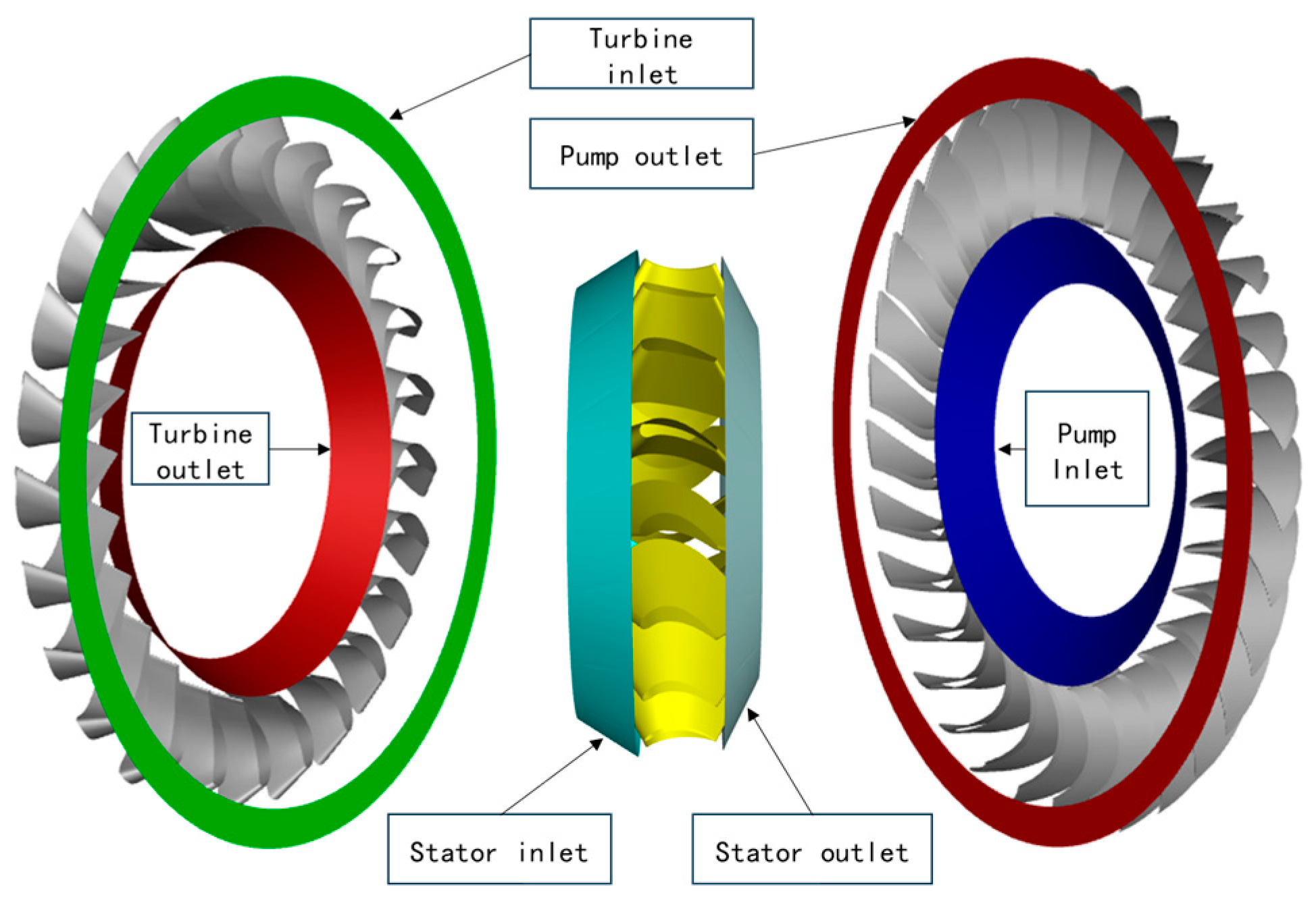
2.2. Geometric Modeling of Torque Converter

The torque converter studied in this paper is a high-power torque converter matching a heavy commercial vehicle, and the specific parameters are shown in

Table 1. Torque converter parameter table.

Rated torque	3500 N·m
Torus diameter	440 mm
Torus width	178 mm
Impeller	Pump	Turbine	Stator
Inlet angle	125.7°	45.8°	121.5°
Outlet angle	48.4°	155.4°	50.56°
Blade number	31	32	17

. Torque converter manufactured by the casting method.

2.3. Simulation Model of Torque Converter

The simulation analysis of hydraulic torque converters involves two calculation models: a two-phase flow model that considers cavitation and a single-phase flow model that does not. The latter can be used to calculate the flow field of a unidirectional flow model without cavitation. The absolute pressure in the results is analyzed to determine whether cavitation occurs or not [16]. For this study, we utilized the impeller-closed flow field model without cavitation and entrance/exit setup. To simplify the model, we ignored any liquid leakage between each impeller and the casting fillet. The full flow channel of the impeller is established, as depicted in Figure 1.

The hexahedral meshing technique is utilized for meshing. To enhance the accuracy of the calculation, boundary layer meshing is applied to refine the near-wall meshes of the pump, turbine, and stator. The height of the first layer mesh was set to 0.0235 mm, with a growth coefficient of 1.25 and a cumulative increase of 10 layers, ensuring that the average y+ value was <2. CFD models with different grid sizes were established to balance the relationship between computational effort and accuracy. Numerical simulations were conducted in stall condition and the zero-speed nominal torque of the pump was extracted for analysis. As shown in

Table 2. Grid independence analysis.

Tot. Elements ($\times {10}^6$)	${\mathit{M}}_{\mathit{B}\mathit{g}0}$ (N·m)	Div./%	Duration (h)
2.59	796.9	-	1.8
3.77	876.9	10.04%	2.5
4.38	949.7	8.30%	3.3
5.31	962.5	1.35%	3.9
7.48	966.2	0.38%	6.5
8.38	968.3	0.22%	11.4

, when the grid quantity increased from 7.48 million to 8.38 million, the calculation error was controlled within 0.3%, while the calculation time significantly increased from 6.5 h to 11.4 h. In consideration of the computational cost and prediction accuracy, the 7.48 million grid cells were employed in this paper. The grid model is illustrated in Figure 2.

The Reynolds-averaged Navier–Stokes equation (RANS) turbulence model and large eddy simulation (LES) are currently the most commonly used turbulence models. RANS is primarily based on the Reynolds time-averaged Navier–Stokes (N-S) equations for solving turbulence problems. It introduces the Reynolds stress term, which is generated by turbulent pulsation velocity in the original N-S equation, providing high accuracy in solving near-wall turbulent motion. On the other hand, LES operates by first spatially filtering the N-S equation and directly simulating large-scale eddies in turbulence using the instantaneous N-S equation. The impact of small eddies on large eddies is accounted for through an approximate sub-grid model. In recent years, hybrid models have been developed, employing the RANS method to solve turbulent boundary layer flow in the near wall region and the LES method in the far-away wall region to enhance computational accuracy [17,18]. The control equation for LES is based on grid size screening and obtained by filtering the N-S function. The filter function is as follows:

$$G\left(\left|x-x^{\prime }\right|\right)=\left\{\begin{array}{c}0\\ \frac{1}{\Delta x_1\Delta x_2\Delta x_3}\end{array}\right.\begin{array}{c}\left|x_i-{x^{\prime }}_i\right|>\frac{\Delta x_i}{2}\left(i=1,2,3\right)\\ \left|x_i-{x^{\prime }}_i\right|\le \frac{\Delta x_i}{2}\left(i=1,2,3\right)\end{array}$$

(2)

$G$ Filter function.

$∆x_i$ The grid scale along the i direction in the coordinate system.

The simulated equation for LES calculation after filtering is as follows:

$$\frac{\partial {\overline{u}}_i}{\partial t}+\frac{\partial {\overline{u}}_i{\overline{u}}_j}{\partial x_j}=-\frac{1}{\rho }\frac{\partial \overline{p}}{\partial x_i}+v\frac{{\partial }^2{\overline{u}}_i}{\partial x_i\partial x_j}-\frac{\partial {\tau }_{ij}}{\partial x_j}$$

(3)

$$\frac{\partial \rho }{\partial t}=-\frac{\partial x}{\partial x_i}\left(\rho {\overline{u}}_i\right)$$

(4)

$u_i,u_j$ Time mean velocity in tensor, m/s.

$v$ Kinematic viscosity coefficient.

$p$ Fluctuation pressure.

${\tau }_{ij}$ The sublattice stress term can be solved by the following equation.

$$\left\{\begin{array}{c}{\tau }_{ij}=\frac{1}{3}{\tau }_r{\delta }_{ij}-2{\mu }_t{\overline{S}}_{ij}\\ {\overline{S}}_{ij}=\frac{1}{2}\left(\frac{\partial {\overline{u}}_i}{\partial x_j}+\frac{\partial {\overline{u}}_j}{\partial x_i}\right)\end{array}\right.$$

(5)

${\delta }_{ij}$ Kronecker delta.

${\overline{S}}_{ij}$ Stress tensor ratio.

${\tau }_r$ Isotropic sublattice stress, Pa.

${\mu }_i$ Sublattice scale turbulent viscosity.

FLUENT offers six sublattice models for the LES model. The Smagorinsky–Lilly (SL) sublattice model, which is currently more widely used, includes the expression for the turbulent viscous coefficient ${\mu }_t$ [19].

$${\mu }_t=\rho {\left\{\mathit{min}(0.41d; C_S{V}^{1/3})\right\}}^2\sqrt{2\overline{S_{ij}}\overline{S_{ij}}}$$

(6)

$d$ Height of the first layer of the grid

$C_s$ SL sub-grid model constant

$V$ Volume of the computational cell

The Shear stress transport (SST) model was employed to solve the boundary layer. When the turbulent scale $L_t$ is smaller than the local grid size, the turbulence switches from the LES model to the SST model. The mixing term for the turbulent kinetic energy equation of the SST model ${\epsilon }_{SDES}$ is presented in the following equation [16];

$$\left\{\begin{array}{c}{\epsilon }_{SDES}=-{\beta }^{*}k\omega F_{SDES}\\ F_{SDES}=\left[max\left(\frac{L_t}{C_{DES}{\Delta }_{SDES}}\left(1-f_s\right),1\right)-1\right]\end{array}\right.$$

(7)

${\beta }^{*}$ Model constants.

$k$ Turbulent kinetic energy.

$\omega$ Turbulence dissipation rate.

$F_{SDES}$ Correction factor.

$L_t$ Turbulent length.

$C_{DES}$ Simulation coefficient of shedding vortex,

${\Delta }_{SDES}$ Grid characteristic length of shedding vortex.

$f_s$ Blending function.

The blending function was applied to accelerate the transition from the RANS turbulence model to the LES turbulence model, which can be obtained by the following equation:

$${\tau }_{ij}^{SBES}=f_s{\tau }_{ij}^{RANS}+\left(1-f_s\right){\tau }_{ij}^{LES}$$

(8)

${\tau }_{ij}^{SBES}$, ${\tau }_{ij}^{RANS}$, ${\tau }_{ij}^{LES}$ The stress tensor in stress-blended eddy simulation, RANS and LES turbulence mode

The turbulence model and boundary condition settings for the flow field calculation are shown in

Table 3. Turbulence modeling and boundary conditions for flow field calculations.

Item	Parameter
Analysis Type	Transient Calculation
Type of fluid domain	Full-flow channel model
Turbulence model	RANS/LES
Mesh type	Hexahedral structured mesh
y+ value	≤2
Density of hydraulic transmission oil	860 kg/m3
Fluid oil viscosity	0.01784 kg/(m·s)
Time step	0.0005 s/step
Simulation time step	400
Pressure-velocity coupling method	SIMPLE
Transient spatial discretization method	Bounded second-order implicit
Other terms spatial discretization	Second-order upwind
Pump rotational speed	1700 r/min
Turbine rotational speed	0–1700 r/min
Stator rotational speed	0 r/min

.

3. Identification of Cavitation in Torque Converter

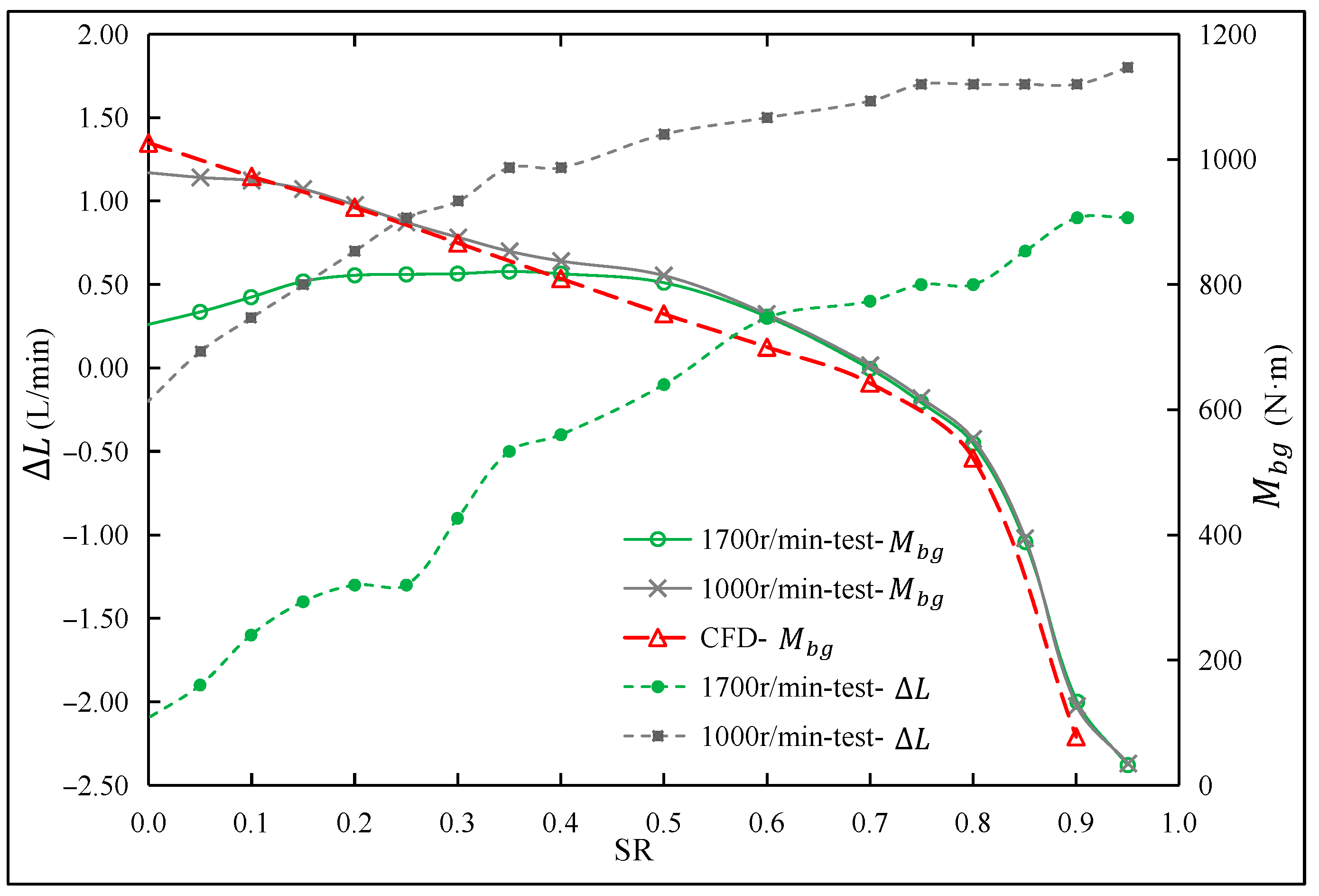
3.1. Cavitation Identification Method Based on Flow Difference

The studies in [9,10,11,12] show that when cavitation occurs in the torque converter, it will produce a large number of cavitation bubbles, some of the cavitation bubbles will disappear and burst inside the torque converter, and some of the bubbles will flow away with the circulating fluid of the torque converter. This part of the bubbles will cause a change in the oil flow rate from the torque converter, so this paper proposes using the cavitation identification method based on the difference between the inlet and outlet flow rate of the torque converter.

Define the flow difference between the inlet and outlet of the torque converter during operation as $∆L$, then

$$\Delta L=L_{in-let}-L_{out-let}$$

(9)

$L_{in-let}$ Torque converter inlet flow (L/min).

$L_{out-let}$ Torque converter outlet flow (L/min).

Under normal working condition, due to the factor of high pressure in the cavity, the torque converter leaks part of the torque converter oil from the matching gap of the oil seal, rotary shaft seal, locking clutch piston and other parts during the working process, so the general $L_{out-let}$ is smaller than the $L_{in-let}$, and the $\Delta L>0$. When cavitation occurs, a large number of cavitation bubbles flow out with the circulation circuit, which causes the outlet flow rate to increase and leads to a decrease or even negative value of the $\Delta L$. If the value of $\Delta L$ decreases or becomes negative, cavitation can be judged by the change in $\Delta L$.

3.2. Test Bench Setup and Test Procedure

The torque converter test bench mainly consists of a drive motor, a load motor, a hydraulic system, a heat exchanger system, a control unit and a detection unit. The torque converter is mounted on the test bench as shown in Figure 3. The detailed parameters of the test bench are shown in

Table 4. Main equipment parameters of torque converter test bench.

Part	Model	Range	Accuracy
Drive motor (VEM Gruppe, Dresden, Germany)	EN60034-1	±2940 r/min; ±7000 N·m	±1 r/min; ±0.1%
Load Motor (Alibaba, Hangzhou, Chian)	FQDI35.5-4WFI	±4500 r/min; ±7200 N·m	±1 r/min; ±0.1%
Torque Sensor (S. Himmelstein and Company, Hoffman Estates, IL, USA)	K-T40B-010R-MF-S	±10,000 N·m	±0.1% F.S.
Encoder (Encoder Products Company (EPC), Sagle, Idaho)	HMCK16 A1 NM02	0–3000 r/min	12 bit
Temperature Sensor (Omega Engineering, Norwalk, NJ, USA)	PT100(AA)	−50–200 °C	±0.5 °C
Pressure Sensor (ESI Technology Ltd., Wrexham, Wales)	1A00QODP5IX	0–3000 kPa	±0.5%

.

During the constant speed test of the torque converter, the pump speed was maintained at a constant 1000 r/min or 1700 r/min, while the turbine speed was varied according to a specific speed ratio [20]. The stall test, on the other hand, was conducted by keeping the turbine speed at or near 0 r/min, and varying the pump speed according to the gradient ratio of 600:100:1700. The obtained data were processed in accordance with Equation (1).

3.3. Identification of Cavitation

The research object was analyzed through constant speed and stall simulations with different pump rotational speeds, following the method described above. At the same time, constant speed and stall tests were conducted with varying pump rotational speed inputs. The results of the simulation and experiment’s constant speed test are presented in Figure 4 and Figure 5, respectively.

As shown in Figure 4, the $TRs$ for input speeds of 1000 r/min and 1700 r/min in the coupled speed ratio region (0–0.8) are nearly identical, with relatively small errors. The distinction between the test $TR$ and the simulated $TR$ is primarily evident in the low speed ratio range of 0–0.2. The most significant difference occurs at a speed ratio of 0.1, with a difference rate of 1.9% for the $TR$. Overall, the difference rate is relatively small. The maximum efficiency ${\eta }_{max}$ at 1000 r/min input speed is slightly decreased by 1.1% compared to the ${\eta }_{max}$ at 1700 r/min input speed, which is 1.8% different from the simulated ${\eta }_{max}$, and the overall rate of difference is small, proving the accuracy of the simulation model. The significant discrepancy in both $TR$ and $\eta$ beyond the 0.8 speed ratio is attributed to the rotation of the stator freewheel after the coupling point during the actual test, which enhances the transmission efficiency.

As shown in Figure 5, the $M_{bg}$ tested at 1000 r/min pump input speed and 1700 r/min pump input speed are the same in the high speed ratio region of 0.5–0.9, with a smaller error. In the low speed ratio region of 0.0–0.4, however, there is a significant difference between the $M_{bg}$ tested at 1000 r/min pump input speed and 1700 r/min pump input speed. This difference rate is inversely proportional to the $SR$, meaning that the lower the $SR$, the larger the difference rate. The $M_{bg0}$ at 1000 r/min input speed is 978.5 N·m, while that of the pump at 1700 r/min input speed is 735.6 N·m. The difference rate of the nominal torque reaches 33%. This phenomenon is caused by the cavitation of the torque converter in conditions of high rotational speed, high load, and low speed ratio, as well as a decrease in the torque of the pump and turbine.

Figure 5 shows the change curve of $∆L$. It is observed that the $\Delta L$ decreases as the $SR$ decreases. In the high speed ratio region, cavitation inside the torque converter occurs less frequently or not at all. The circulating fluid enters the torque converter and exits after a certain leakage, resulting in a larger inlet flow rate than the outlet flow rate, and a positive value for the $\Delta L$. As the speed ratio decreases and cavitation occurs, a large number of bubbles flow out with the circulating circle, resulting in an increase in the outlet flow. This leads to a decrease in the $\Delta L$ or even a negative flow difference. At a pump speed of 1000 r/min and a speed ratio of 0.9, the $\Delta L$ is 1.8 L/min, with a stall condition of −0.2 L/min. At a pump speed of 1700 r/min and a speed ratio of 0.9, the $\Delta L$ is 0.9 L/min, with a stall condition of −2.1 L/min. The phenomenon of cavitation becomes more pronounced as the $SR$ decreases and the pump speed increases.

Figure 6 shows the results of the stall test performed at different pump speeds. The $M_{bg0}$ tends to increase initially and then decrease rapidly with the increase in pump speed, as shown in comparison with the simulation value. This is due to the fact that at low pump speeds, the hydraulic converter’s oil viscous friction loss accounts for a significant portion of the total loss, resulting in a relatively low $M_{bg0}$ of the pump wheel. As the speed of the pump wheel increases, the degree of cavitation also increases. This causes the medium acting on the impeller to evolve from pure hydraulic oil to a gas–liquid two-phase mixture. As a result, the force on the impeller weakens, leading to a sharp decline in the $M_{bg0}$ of the torque converter. The $\Delta L$ between the inlet and outlet of the torque converter and the changing trend of $M_{bg0}$ are similar.

According to the analysis above, the hydrodynamic torque converter experiences cavitation in the large load region with high speed and low speed ratio, resulting in a decrease in $M_{bg}$. The $\Delta L$ of the hydrodynamic torque converter can be used to determine if cavitation is occurring. It can be determined that cavitation has occurred in this torque converter when $\Delta L\le 0 \mathrm{L}/\mathrm{m}\mathrm{i}\mathrm{n}$.

4. Optimized Design of Cavitation in High Power Torque Converter

The stator plays a crucial role in the working process of the torque converter. Its main function is to withstand the turbine outflow with the energy of the ATF oil. This counteracts the impact of the hydraulic oil on the turbine, promoting the turbine output torque. Additionally, it forces the flow direction of the hydraulic oil speed impact angle commutation, directing it towards the pump wheel to avoid any impact on it [21].

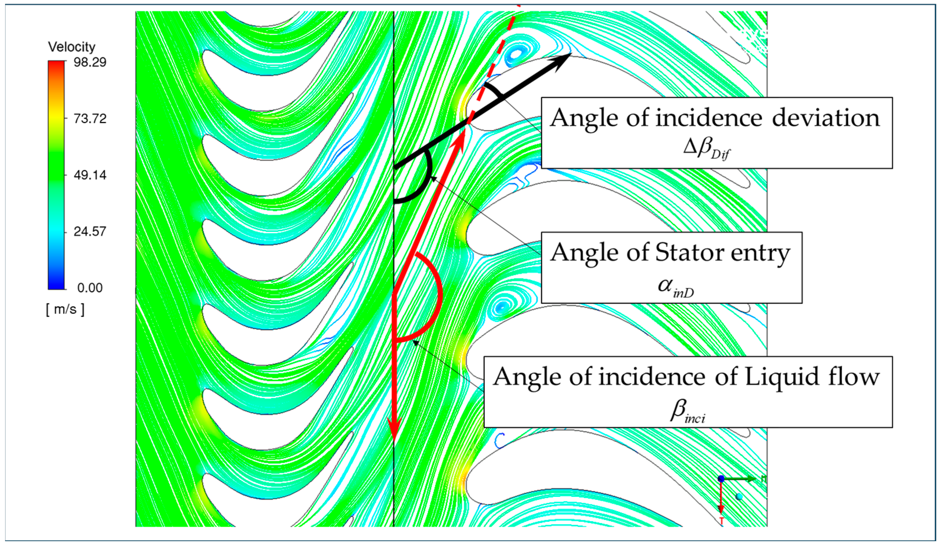
4.1. Analysis of Cavitation Mechanism of Hydraulic Torque Converter

The pressure surface is defined as the side of the stator facing the impact of the liquid flow, while the suction surface is defined as the other side. A simulation calculation was performed on the research object with an input speed of 1700 r/min and a speed ratio of 0 for the pump wheel. After the calculation was completed, the pressure and velocity cloud diagram of the stator was extracted, as shown in Figure 7.

Under the initial conditions, negative pressure was observed on the surface of the stator blades due to the lack of consideration of cavitation. The lowest negative pressure on the stator blade surface $P_{lowest\_D}$ was −2.76 MPa as shown in Figure 7a. The negative pressure region was mainly located at the starting position of the suction surface of the stator blades, specifically the side of the suction surface at the nose of the stator. Meanwhile, a low-pressure region, which is a localized vortex region as shown in Figure 7d, is distributed above the front suction surface at the peak bending position of the stator. The lowest pressure, denoted as $P_{lowest\_D}$ of the stator occurs in the nose region of the stator, specifically located on the pressure surface side of the nose region. This region is directly impacted by the turbine hydrodynamics.

The velocity cloud diagram shows that the flow velocity near the stator blade region is nearly zero due to the viscous effect of the liquid flow near the wall. Some of the liquid flow moves towards the pressure surface of the stator, while another part of the velocity increases rapidly after skimming over the nose region of the stator. The velocity then levels off after entering the middle region of the blade. Regions of low-velocity flow with varying degrees can be observed above the front suction surface at the peak position of stator bending. Figure 7c shows that the liquid flow impacts the pressure surface adjacent to the stator blades after skimming the nose of the stator. The flow then folds back to form a vortex, which is the main factor causing the emergence of local negative pressure and local low-speed flow region above the front suction surface at the peak position of the stator bending.

As shown in Figure 8, the angle between the turbine liquid flow outflow direction vector and the rotation direction vector of the impeller in the stall condition is defined as the stator liquid flow incidence angle ${\beta }_{inci}$, and the angle between the stator liquid flow incidence angle ${\beta }_{inci}$ and the stator blade streamlined inlet angle ${\alpha }_{inD}$ is defined as the liquid flow incidence deviation angle $\Delta {\beta }_{Dif}$.

$$\Delta {\beta }_{Dif}={\beta }_{inci}-{\alpha }_{inD}$$

(10)

Figure 7d shows the partial diagram of the stator streamline. In stall conditions, the $\Delta {\beta }_{Dif}$ formed by the turbine outlet angle and the inlet angle of the stator nose is larger, resulting in high-speed liquid flow being swept over the stator nose flow to the suction surface of the liquid flow being greater. In the stator nose and the stator, bending the peak position of the front of the suction surface over the formation of a localized negative pressure zone, respectively, is the cause of the occurrence of cavitation in the torque converter.

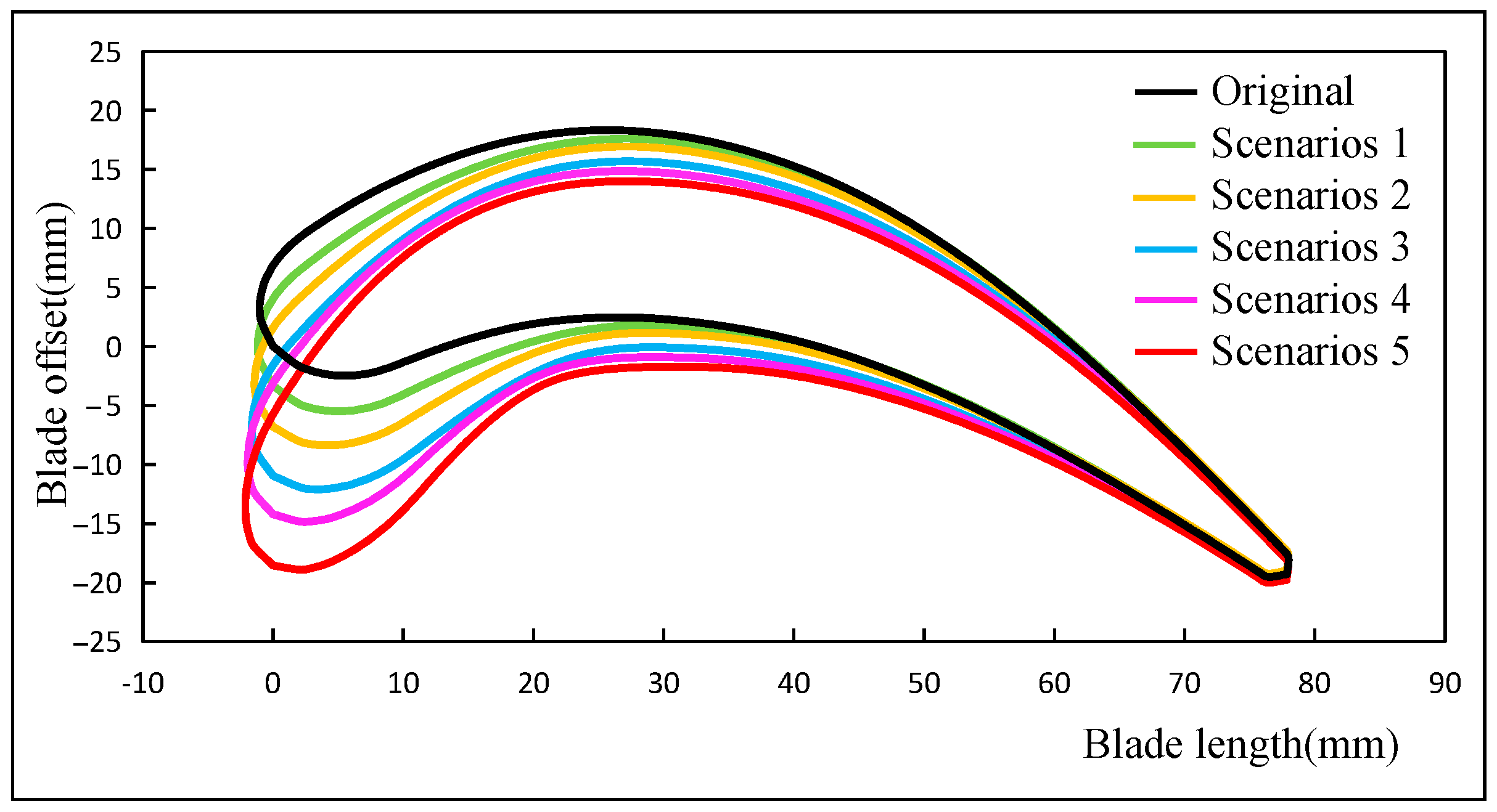
4.2. Optimized Design of Torque Converter Stator

The design parameters of the stator are mainly divided into mean camber line parameters and thickness parameters. The mean camber line parameters are inlet angle ${\alpha }_{inD}$, outlet angle ${\alpha }_{outD}$, blade camber line deflection angle ${\gamma }_D$, peak position coefficient position coefficient $x_{hD}$, peak height coefficient $y_{hD}$, and chord length $L_D$ [22]. The thickness and mean camber line parameters are similar and will not be repeated, as shown in Figure 9.

Currently, there are more studies on the relationship between the mean camber line parameters of the stator and the torque converter performance, but fewer studies on their relationship with cavitation. To investigate the impact of stator nose characteristics on cavitation, the ${\alpha }_{inD}$, ${\gamma }_D$, $x_{hD}$, $y_{hD}$, and $L_D$ were varied to achieve different $\Delta {\beta }_{Dif}$. The ${\alpha }_{outD}$ was kept constant and the shape of the back half of the blade peak remained unchanged. Six schemes (1–6) were formed as shown in

Table 5. Design parameters for different scenarios.

Item	Parameter
Angle of incidence deviation of flow injection $\Delta {\beta }_{Dif}$ (°)	original	34.66	scenarios 3	19.66
	scenarios 1	25.16	scenarios 4	17.16
	scenarios 2	21.16	scenarios 5	14.16
Outlet angle ${\alpha }_{outD}$ (°)	50.56
inner ring offset (rad)	0.097
chord length $L_D$ (mm)	77.82

.

The 2-D blades of different schemes are shown in Figure 10, from which it can be seen that by adjusting the parameters, the ${\alpha }_{outD}$ of the blade, the shape of the second half of the peak of the blade is basically unchanged, while the shape of the head of the stator blades has undergone a major change, and the turbine exit angle of the liquid flow forms a different degree of $\Delta {\beta }_{Dif}$.

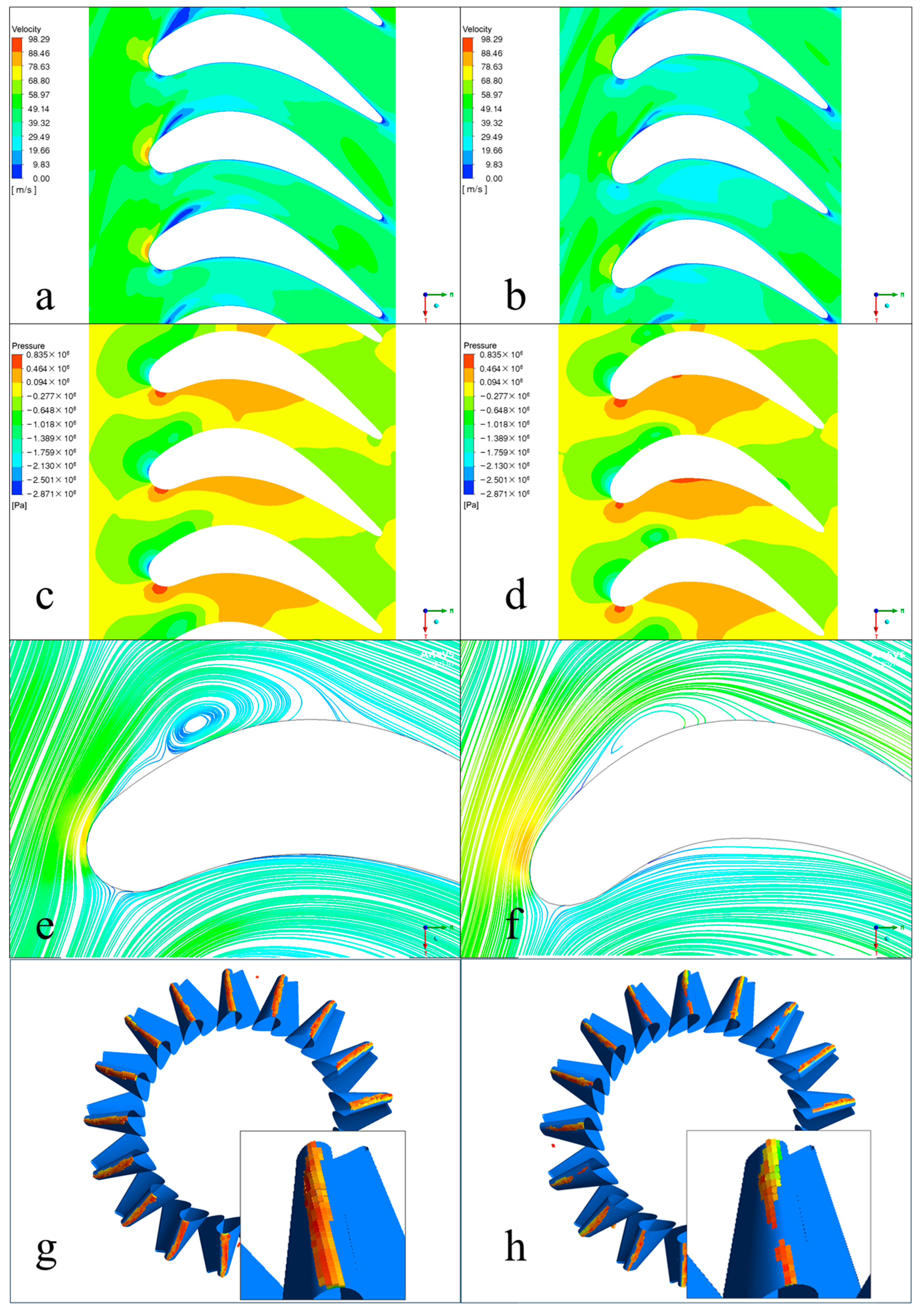
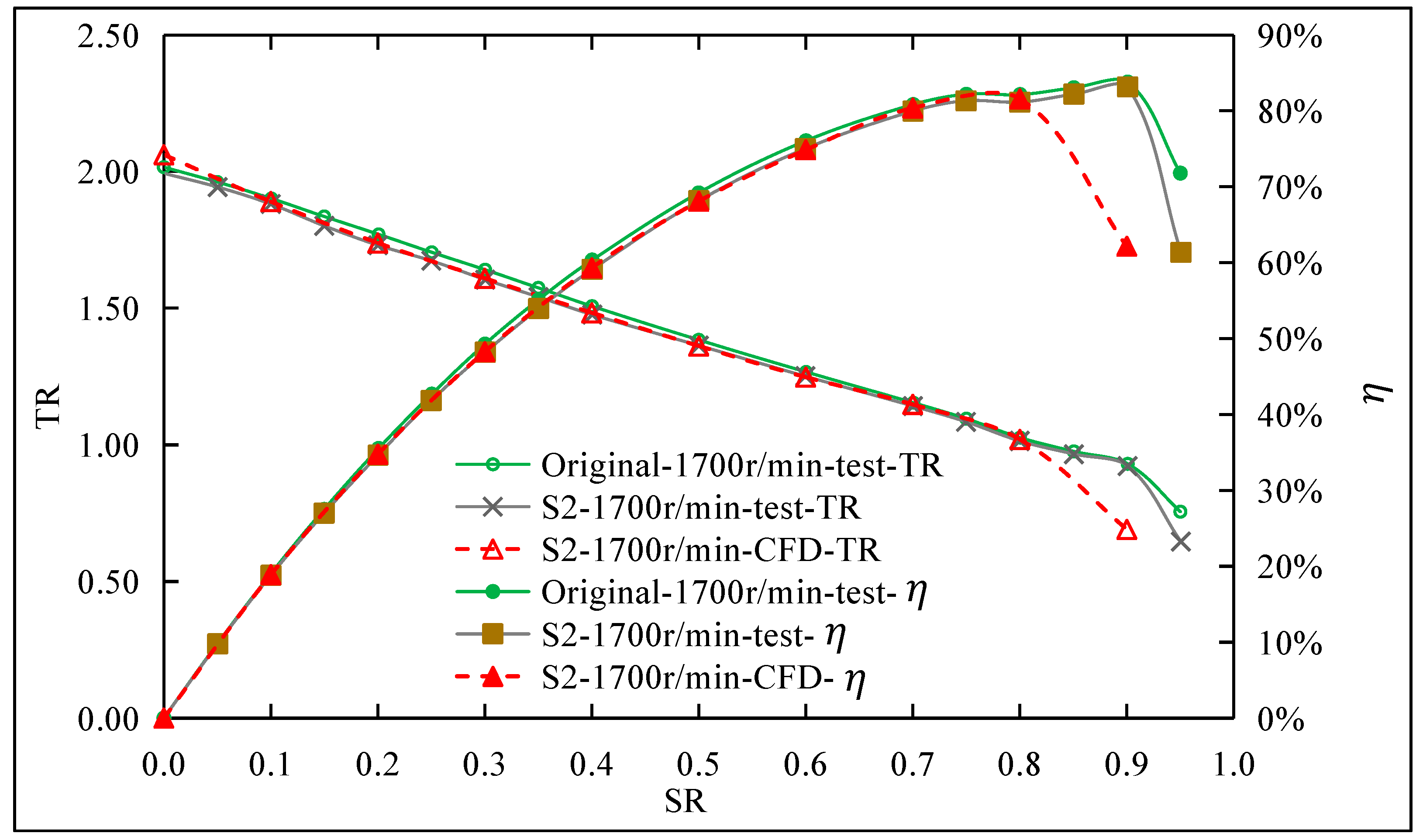
4.3. Simulation Analysis of Torque Converter Stator Optimization Scheme

The optimized stator is discretized into a hexahedral mesh and set up for simulation according to Table 2, and the pump input speed is 1700 r/min for zero-speed stall simulation. The relationships between the $\Delta {\beta }_{Dif}$ and $TR$, $P_{lowest\_D}$, $M_{bg0}$ and $M_T$ are plotted as shown in Figure 11.

From Figure 11, it can be seen that the $TR$, $M_{bg0}$ and $M_T$ all have quadratic functional relationships with $\Delta {\beta }_{Dif}$, and the $P_{lowest\_D}$ and $\Delta {\beta }_{Dif}$ have approximately primary functional relationships. The specific relation equation is as follows.

$$P_{lowest}=-0.0266\cdot \Delta {\beta }_{Dif}-2.5062$$

(11)

$$K=-0.0008\cdot {\Delta \beta }_{Dif}^2+0.0444\cdot \Delta {\beta }_{Dif}+1.4633$$

(12)

$$M_{Bg}=0.8111\cdot {\Delta \beta }_{Dif}^2-46.573\cdot \Delta {\beta }_{Dif}+1663.3$$

(13)

$$M_T=2.1\cdot {\Delta \beta }_{Dif}^2-128.85\cdot \Delta {\beta }_{Dif}+7907.4$$

(14)

Figure 11a shows that the $TR$ of the hydraulic torque converter tends to increase and then decrease with an increase in $\Delta {\beta }_{Dif}$. The difference rate between the maximum and minimum values of the $TR$ is 6.8%, which is relatively low. It is important to note that this analysis is based solely on objective data and does not include any subjective evaluations. The minimum pressure on the surface of the stator blades tends to increase with an increased $\Delta {\beta }_{Dif}$. The difference rate between the maximum and minimum values of the minimum pressure is 20.4%. The $M_{bg0}$ exhibits a downward and then upward trend as the $\Delta {\beta }_{Dif}$ increases. The difference rate between the maximum and minimum values of $M_{bg0}$ is 15.3%. The change in $\Delta {\beta }_{Dif}$ is more significant for the $P_{lowest\_D}$ of the hydrodynamic torque converter and $M_{bg0}$, which are the most important factors in the optimization. $M_{bg0}$ has a large effect, while the effect on $TR$ is small. The analysis of the results of the comprehensive optimization scheme reveals that the $P_{lowest\_D}$ in the zero-speed condition of Scheme 2 is improved from −2.78 MPa to −2.29 MPa, which is 17.6%, while the $TR$ is improved from 2.017 to 2.040, with a change rate of 1.14%, the $M_{bg0}$ is reduced from 1020.8 N·m to 1008.1 N·m, with a change rate of 1.24%, and Scheme 2 significantly optimizes the $P_{lowest\_D}$ on the surface of the stator while basically keeping the basic performance unchanged, which can be taken as the preferred scheme.

Figure 12 presents a comparison between the simulation results of the original scheme and Scheme 2. As shown in Figure 12a,b, the optimized liquid flow velocity through the stator decreases at the highest velocity in the region where the velocity rapidly increases and sweeps over the nose of the stator, with a decrease rate of 13.5%. Additionally, the low-speed flow region above the front suction surface at the peak position of the stator bending disappears, and the majority of the low-speed region is now close to the surface of the blade. The vortex above the front suction surface at the peak stator bending position is weakened or disappears.

Figure 12c–f display the pressure cloud and localized liquid flow vectors in the nose region of the stator in both the original scheme and Scheme 2. The pressure cloud and liquid flow vector cloud indicate that a smaller liquid inflow deviation angle, $\Delta {\beta }_{Dif}$, leads to a better fit between the shape of the stator’s nose in the stalled condition and the liquid inflow angle, ${\beta }_{inci}$. This, in turn, significantly reduces vortices above the forward suction surface at the peak location of the stator bending. Figure 12e,f show a significant reduction in the optimized low-pressure distribution region, which is below the cavitation pressure of the hydrodynamic oil. Scheme 2 optimizes the $P_{lowest\_D}$ while maintaining basic performance.

The external characteristic diagram of the torque converter resulting from further simulation analysis of Scheme 2 in the full-speed domain is shown in Figure 13. It can be observed that the maximum rate of difference between the $TR$ of the optimized Scheme 2 and that of the original scheme is 2.55% at 0.1 $SR$ in the speed domain the range of 0–0.8. Additionally, the maximum rate of difference of the $M_{bg}$ is 7.08% at 0.8 $SR$. In the low speed ratio region, the maximum difference rate of $M_{bg}$ is only 3.53%. At a speed ratio of 0.8, the maximum difference rate of η is 1.89%. In the high speed ratio region of ≥0.5, the $\eta$ of Scheme 2 is slightly lower than the original scheme. Overall, the new scheme maintains the same external characteristics as the original scheme. However, the stator’s cavitation characteristics have been greatly improved.

5. Validation of Cavitation Optimization for High Power Torque Converter

The stator for Scheme 2 was 3D printed using the results of the first optimization calculations to verify their accuracy. Figure 14 compares the original stator with the new design for Scheme 2.

The design of the stator blades was optimized and tested with the original torque converter’s impellers, the turbine, and the pump wheel, while the stator was updated to the Scheme 2 design stator. The torque converter was tested at a constant speed to obtain test results for the new torque converter assembled with the original scheme torque converter and the Scheme 2 stator, ensuring that the test input conditions (system pressure, flow rate, etc.) were consistent with the original scheme test conditions. The obtained results are shown in Figure 15.

As shown in Figure 15, the new hydraulic torque converter scheme exhibits a slight decrease in the overall $TR$ when compared to the original scheme, with a maximum difference rate of 2.31%. Additionally, the ${\eta }_{max}$ generally decreases, with a maximum decrease of 0.9 percentage points. However, this change maintains the consistency of the torque converter’s $TR$ and ${\eta }_{max}$.

Figure 16 shows that the $M_{bg}$ at 1700 r/min pump input speed measured by the original scheme and Scheme 2 are almost identical with a small error in the speed ratio with an interval of 0.4–0.9. However, in the low speed ratio region of 0.0–0.4, the $M_{bg}$ of the hydrodynamic torque converter is significantly improved. The $M_{bg0}$ is improved from the original 735.6 N·m to 946.8 N·m, resulting in a 28.7% improvement rate.

The change curve of $\Delta L$ in Figure 16 shows that cavitation occurs in the original scheme when the $SR$ is below 0.5 and exacerbates as the $SR$ decreases; the flow difference, $\Delta L$, is −2.1 L/min in stall conditions. The $\Delta L$ of Scheme 2 has been significantly improved and only slight cavitation occurs when the speed ratio is ≤0.15. The $M_{bg}$ is not affected significantly compared to the simulation data. These improvements greatly reduce cavitation in the hydrodynamic torque converter.

6. Discussion

This paper presents a study on the phenomenon of cavitation in high-power hydraulic torque converters. Firstly, a transient flow field model of the torque converter was established. Then, CFD simulation analysis and experimental research were conducted on the torque converter. Finally, a cavitation identification method based on the difference between the flow rate of the inlet and outlet of the torque converter was proposed. The analysis focused on the transient flow process within the torque converter. It was found that the angle between the stator’s inlet and the turbine’s outlet is a crucial factor in the occurrence of cavitation. An optimized design was then implemented.

The angle of incidence deviation of flow injection, $\Delta {\beta }_{Dif}$, is formed by the liquid flow angle out of the turbine and the inlet angle of the stator nose during stall conditions. This angle is larger, resulting in more high-speed liquid flow skimming over the nose of the stator and onto the suction surface. This creates a localized negative pressure zone above the front suction surface at the peak position of the stator nose and the stator bending, respectively. This is the main reason for cavitation occurring in the hydrodynamic torque converter. The occurrence of cavitation in the torque converter can be determined by the difference in inlet/outlet flow ($\Delta L$). In the case of this torque converter, cavitation can be identified when the $\Delta L$ ≤ 0 L/min.

Cavitation mainly occurs in the torque converter at high pump input speeds and under large load conditions with low speed ratios. At lower pump input speeds, even with lower speed ratios, cavitation is less likely to occur. In the low speed ratio region (0–0.5) under high pump input speed conditions, cavitation occurs in the torque converter and tends to be strengthened with decreasing speed ratios.

Cavitation mainly affects the capacity of the torque converter, specifically the $M_{bg}$, and has less impact on the torque ratio and efficiency of the converter. The $M_{bg0}$ of the pump wheel at 1000 r/min is 978.5 N·m, while that of the pump wheel at 1700 r/min is 735.6 N·m, resulting in a 33% difference in $M_{bg0}$. It is important to note that this difference rate of $M_{bg0}$ reaches 33%.

A series of stator optimization design schemes were developed by changing the $\Delta {\beta }_{Dif}$ of the torque converter. The aim was to identify the variation rules of $TR$, $P_{lowest\_D}$, $M_{bg}$, and $\Delta {\beta }_{Dif}$. It was found that Scheme 2 optimizes the $P_{lowest\_D}$ significantly while keeping the performance of the zero-speed startup condition basically unchanged. The optimized Scheme 2 has maximum difference rates of $TR$, $M_{bg}$, and $\eta$ controlled within 8%, while maintaining the same external characteristics as the original scheme.

Tests were conducted on the stator of Scheme 2 using 3D rapid printing and mounting. The new hydraulic torque converter scheme showed a slight decrease in the overall $TR$ compared to the original design, with a maximum difference rate of 2.31%. The ${\eta }_{max}$ was also generally decreased, with a maximum decrease of 0.9 percentage points. However, this maintained the consistency of the torque converter’s $TR$ and $\eta$. The hydrodynamic torque converter’s $M_{bg0}$ was significantly improved from 735.6 N·m to 946.8 N·m, resulting in a 28.7% improvement rate. Additionally, the cavitation region shrunk from 0–0.5 to 0–0.15, resulting in a significant improvement in the torque converter’s cavitation phenomenon.

The paper proposes an optimization method for cavitation in torque converters, which can also be applied to optimize the design of other high-power torque converters with similar working conditions. This method provides a new design idea for high-power torque converters to reduce transmission loss and improve reliability. The insights obtained from studying cavitation in torque converters can be effectively transferred to other engineering systems where cavitation is significant, such as hydraulic systems, pumps, propellers, and turbines. This broad applicability across industries enhances the importance and relevance of research conducted in this field.

References

1. Chen, J.; Wu, G. Kriging-assisted design optimization of the impeller geometry for an automotive torque converter. Struct. Multidiscip. Optim. 2018, 57, 2503–2514. [Google Scholar] [CrossRef]
2. Yang, Y.; Liou, W.W.; Qureshi, F.; Whitticar, D.J.; Michael, E.H. Transmission fluid properties’ effects on performance characteristics of a torque converter: A computational study. Tribol. Trans. 2021, 64, 1055–1063. [Google Scholar] [CrossRef]
3. Xiong, P.; Sun, H.; Zhong, J.; Zhen, C.; Chen, X.; Gao, H. Analysis of the Influence of the Number of Torque Converter Blades on Working Performance Based on the Response Surface Method. J. Phys. Conf. Ser. 2021, 1748, 022028. [Google Scholar] [CrossRef]
4. Wang, G. Research on Scale-Resolving Simulation for Flow Field and Cavitation Characteristics of Hydrodynamic Torque Converter. Ph.D. Thesis, Jilin University, Changchun, China, 2022. (In Chinese). [Google Scholar]
5. De Jesus Rivera, E. Pressure Measurements Inside Multiple Cavities of a Torque Converter and CFD Correlation. Ph.D. Thesis, Michigan Technological University, Houghton, MI, USA, 2018. [Google Scholar]
6. Ju, J.; Jang, J.; Choi, M.; Baek, J.H. Effects of cavitation on performance of automotive torque converter. Adv. Mech. Eng. 2016, 8, 1687814016654045. [Google Scholar] [CrossRef]
7. Guo, M.; Liu, C.; Liu, S.; Ke, Z.; Wei, W.; Yan, Q.; Khoo, B.C. Detection and evaluation of cavitation in the stator of a torque converter using pressure measurement. Phys. Fluids 2022, 34, 045124. [Google Scholar] [CrossRef]
8. Tsutsumi, K.; Watanabe, S.; Tsuda, S.-I.; Yamaguchi, T. Cavitation simulation of automotive torque converter using a homogeneous cavitation model. Eur. J. Mech. B/Fluids 2017, 61, 263–270. [Google Scholar] [CrossRef]
9. Zhao, L. The Cavitation Research of the Flow Field in the Hydraulic Torque Converter Based on CFD. Ph.D. Thesis, Taiyuan University of Science and Technology, Taiyuan, China, 2016. (In Chinese). [Google Scholar]
10. Craig, D.R. Characterization of Torque Converter Cavitation Sound Power Level over Varying Speed Ratio. Ph.D. Thesis, Michigan Technological University, Houghton, MI, USA, 2016. [Google Scholar]
11. Chad, M.W. Torque Converter Turbine Noise and Cavitation Noise over Varying Speed Ratio. Ph.D. Thesis, Michigan Technological University, Houghton, MI, USA, 2012. [Google Scholar]
12. Liu, C.; Wei, W.; Yan, Q.; Weaver, B.K.; Wood, H.G. On the application of passive flow control for cavitation suppression in torque converter stator. Int. J. Numer. Methods Heat Fluid Flow 2019, 29, 204–222. [Google Scholar] [CrossRef]
13. Li, J. Investigation on Scale-Resolving Simulation of Unsteady Cavitation Flow around Blades and Its Bionic Control Mechanism. Ph.D. Thesis, Jilin University, Changchun, China, 2022. (In Chinese). [Google Scholar]
14. Xiong, P.; Chen, X.; Sun, H.; Zhong, J.; Wu, L.; Gao, H. Effect of the blade shaped by Joukowsky airfoil transformation on the characteristics of the torque converter. Proc. IMechE Part D J. Automob. Eng. 2021, 235, 3314–3321. [Google Scholar]
15. Ran, Z.; Ma, W.; Liu, C. 3D Cavitation Shedding Dynamics: Cavitation Flow-Fluid Vortex Formation Interaction in a Hydrodynamic Torque Converter. Appl. Sci. 2021, 11, 2798. [Google Scholar] [CrossRef]
16. Liu, C.; Yan, Q.; Li, J.; Li, J.; Zou, B. Investigation on the Cavitation Characteristics of High Power-density Torque Converter. J. Mech. Eng. 2020, 56, 147–155. (In Chinese) [Google Scholar]
17. Song, J.; Bai, H.; Cheng, B.; Zhang, N.; Zhang, W.; Leng, H.; Zhao, W.; Zhang, Z. A review of large eddy simulation of aviation turbulence. Acta Aerodyn. Sin. 2023, 41, 26–43. (In Chinese) [Google Scholar]
18. Wu, T.; Shi, B.; Wang, S.; Zhang, X.; He, G. Wall-Model For Large-Eddy Simulation And Its Applications. Chin. J. Theor. Appl. Mech. 2018, 50, 453–466. (In Chinese) [Google Scholar]
19. Ran, Z.; Ma, W.; Liu, C.; Li, J. Multi-objective optimization of the cascade parameters of a torque converter based on CFD and a genetic algorithm. J. Automob. Eng. 2021, 8, 2311–2323. [Google Scholar] [CrossRef]
20. Ran, Z.; Ma, W.; Wang, K.; Chai, B. Multi-Objective Optimization Design for a Novel Parametrized Torque Converter Based on an Integrated CFD Cascade Design System. Machines 2022, 10, 482. [Google Scholar] [CrossRef]
21. Liu, C.; Xu, Z.; Ma, W.; Wang, S. CFD investigating medium-temperature in fluences on performance prediction and structure stress calculation in a hydrodynamic torque converter. Numer. Heat Transf. Part A Appl. 2017, 72, 563–578. [Google Scholar] [CrossRef]
22. Liu, C.; Wei, W.; Yan, Q. Three Dimensional Torque Converter Blade Modelling Based on Bezier Curves. J. Mech. Eng. 2017, 53, 201–208. [Google Scholar] [CrossRef]
Figure 1. Torque converter CFD modeling.
Applsci 14 04240 g001
Figure 2. Structural mesh model of the hydrodynamic torque converter.
Applsci 14 04240 g002
Figure 3. Torque converter test bench.
Applsci 14 04240 g003
Figure 4. Comparison of the η and T R between the simulation and the test.
Applsci 14 04240 g004
Figure 5. Comparison of M b g and L .
Applsci 14 04240 g005
Figure 6. Performance of the stall test was evaluated at various pump input speeds.
Applsci 14 04240 g006
Figure 7. Simulation cloud map of the original scheme: (a) stator pressure cloud map; (b) stator velocity cloud map; (c) streamline diagram of stator flow direction; (d) localized view of the stator streamline.
Applsci 14 04240 g007
Figure 8. Schematic diagram of liquid flow injection deviation angle.
Applsci 14 04240 g008
Figure 9. Parameterized 2D blade profile.
Applsci 14 04240 g009
Figure 10. Two-dimensional profiles of blades for different scenarios.
Applsci 14 04240 g010
Figure 11. Simulation results of zero-speed conditions for different schemes: (a) relationship between T R and Δ β D i f ; (b) relationship between P l o w e s t _ D and Δ β D i f ; (c) relationship between M b g 0 and Δ β D i f ; (d) relationship between M T and Δ β D i f .
Applsci 14 04240 g011
Figure 12. Comparison of simulation results of optimization schemes: (a) velocity cloud of the stator for the original scheme; (b) velocity cloud of the stator for the optimized scheme; (c) local pressure map of the original scheme; (d) local pressure map of the optimized scheme; (e) original scheme streamline map; (f) optimized scheme flow streamline map; (g) original scheme the low-pressure distribution cloud; (h) optimized scheme the low-pressure distribution cloud.
Applsci 14 04240 g012
Figure 13. Comparison of torque converter simulation performance before and after optimization.
Applsci 14 04240 g013
Figure 14. Comparison of stator samples from the two schemes.
Applsci 14 04240 g014
Figure 15. Comparison of η and T R between simulation and test of optimized scheme 2 (S2).
Applsci 14 04240 g015
Figure 16. Comparison of M b g and Δ L between simulation and test of the optimized scheme.
Applsci 14 04240 g016