Numerical Analyses of the Effect of the Freezing Wall on Ground Movement in the Artificial Ground Freezing Method

Abstract

The advancement of massive construction in urban subway projects contributes to the increased use of the artificial ground freezing (AGF) method in the construction of cross passages due to its reliability and environmental friendliness. However, the uplift or subsidence of the ground surface induced by the frost heave and thawing settlement of the soil can be a problem for existing buildings, and the current design method places way too much emphasis on the strength requirement of the freezing wall. In this study, FLAC3D was employed to develop a series of state-of-the-art numerical models of the construction of a typical subway cross passage by the AGF method, utilizing freezing walls with different thicknesses. The results of this study can be used to examine the ground deformation arising from the AGF method and the influence of the thickness of the freezing wall on the AGF method.

1. Introduction

Over the last decade, the artificial ground freezing (AGF) method, which was originally applied in mining engineering, has been extensively applied in the massive construction of sub-railways in China due to its sterling performance in terms of waterproofing, structure stabilizing, and environmental friendliness [1]. Among the design factors of the AGF method, the most pivotal is the determination of the thickness of the freezing wall, which is highly related to the stability of the excavation and the deformation of the ground surface [2]. In past mining engineering practice, the prevalent method for the determination of the thickness of the freezing wall was the plane-strain elastic–plastic method proposed by Domke [3]. However, considerable research and field practice have shown that the design method employed in mining engineering seems to be inappropriate for the design of urban tunnel excavations, and more considerations of the displacement aspect are needed [4]. In the water supply project that crosses the Yangtze River at Xinjizhou, Jiangning, Nanjing, diverting water from Xinjizhou Island to the pump station at Jiangning District, the AGF method is planned to be adopted for the construction of tunnels. The effects of freezing walls on ground movement need to be evaluated.

This study aims to first investigate the influence of the thickness of the freezing wall on the displacement development characteristics of the freezing and thawing process, examine the temperature distribution within freezing walls with different thicknesses at the selected indicative time points of the characteristic period, and finally evaluate the influence of the thickness of the freezing wall on the ground displacement characteristics. Due to its accuracy and powerful ability to carry out thermal–mechanical coupling analyses, the finite volume program FLAC3D utilizing the three-dimensional explicit Lagrangian method was employed in this study to simulate a set of numerical analyses to model the construction of a subway cross passage using the AGF method with freezing walls of different thicknesses. These numerical analyses are expected to shed light on the thermal–mechanical behavior of freezing walls with different thicknesses, i.e., the frost heave and thaw settlement induced by the freezing wall.

2. Literature Review

Over the past two decades, a great number of researchers have sought new ways to efficiently design freezing walls for the AGF method of subway construction. Yue et al. [5] introduced the widely employed structural mechanics method, which simplifies the freezing wall into an elastic, statically indeterminate structure. Modifying the assumptions, many researchers made improvements to these methods [6,7,8,9]. Despite its safety and efficacy, the structural mechanics method suffers from several major drawbacks: (1) this method is limited to the elastic regime of the material, and the cohesion between unfrozen soil and frozen soil is omitted, which leads to a more conservative design of freezing wall thickness; (2) the thickness of the freezing wall is primarily determined by the strength requirement, with little concern for the deformation of the ground surface caused by freezing heave or thaw settlement; and (3) little attention has been paid to thermal dynamics problems during the development of freezing walls [2,10,11,12,13]. Noting the limitations of the structural analytical method, some scholars tried to develop analytical solutions for predicting the deformation of the ground surface. However, the equations derived are only applicable to limited configurations and have relatively complicated forms [14,15]. Thus, many researchers made an attempt to examine freezing walls using numerical simulation methods. Zhang and He [16], employing the three-dimensional finite element numerical simulation method, carried out research on the mechanical behaviors of the freezing wall during the excavation. Their observation showed that the bottom of the freezing wall had the largest tension zone area. Employing finite element modeling, Fu et al. [17] evaluated temperature field variations during artificial freezing and observed the potential factors affecting the changes in temperature. They found that thermal conductivity had the most significant impact on the development of the temperature field, while the phase-change latent heat had little impact. Huang et al. [18] undertook a study utilizing the COMSOL multi-physical platform to optimize the distribution of the freezing pipes. While the numerical simulation method has been applied to either solely mechanical or purely thermal dynamic problems when modeling freezing walls, research works on the thermal–mechanical problems induced by freezing walls, i.e., frost heave and thaw settlement, remain scarce. Based on a metro entrance construction project, Zhang et al. [19] investigated time variations in frost heave and found that intermittent freezing could effectively control surface deformation. Through laborary model tests in combination with numerical simulations, Cai et al. [20] examined frost heave during twin-tunnel construction; the results showed that sequential freezing could bring about less frost heave displacement than that of simultaneous freezing.

3. Basic Theory for Thermal–Mechanical Calculations

In FLAC3D, thermal dynamic problems are solved by coupling the energy balance equation and transport laws at the specific boundaries and initial conditions given. The equations and boundaries are summarized as follows:

3.1. Energy Balance Equation

The temperature calculation process follows the law of conservation of energy, and the energy balance differential equation has the following form, as shown in Equation (1):

$$-q_{i,i}+q_v=\frac{\partial \zeta }{\partial t}$$

(1)

where q_i,i is the heat-flux vector, q_v is the volumetric heat-source intensity, ζ is the heat stored per unit volume, and t is the time.

In general, changes in both energy storage and volumetric strain, ϵ, can result in a change in the temperature, and the thermal constitutive equation describing this relationship can be expressed as Equation (2):

$$\frac{\partial T}{\partial t}=M_{th}\left(\frac{\partial \zeta }{\partial t}-{\beta }_{th}\frac{\partial ϵ}{\partial t}\right)$$

(2)

where M_th and β_th are material constants, T is temperature, ϵ is the volumetric strain, and the other variables are the same as those mentioned above.

In FLAC3D, the strain changes are thought to have a minimal impact on temperature, which is valid for solid and liquid matter. This assumption leads to a simplification of Equation (2) into Equation (3):

$$\frac{\partial \zeta }{\partial t}=\rho C_v\frac{\partial T}{\partial t}$$

(3)

where ρ is the mass density of the medium, C_v is the specific heat at constant volume, and the other variables are the same as those mentioned above.

Substituting Equation (3) into Equation (1) yields Equation (4):

$$-q_{i,i}+q_v=\rho C_v\frac{\partial T}{\partial t}$$

(4)

where the variables are the same as those in the equations above.

3.2. Transport Law

Fourier’s law links the heat-flux vector to the temperature gradient. For a stationary, homogeneous, isotropic solid, this law can be expressed as Equation (5):

$$q=-k\nabla T$$

(5)

where q is the heat-flux vector, k is the thermal conductivity, and ∇T is the temperature gradient.

3.3. Thermal Boundary Conditions

In FLAC3D, four types of conditions are considered: (1) given temperature; (2) given component of the flux normal to the boundary; (3) convective boundaries; and (4) insulated (adiabatic) boundaries. In FLAC3D, boundaries are adiabatic by default.

3.4. Mechanical–Thermal Coupling

Solutions to thermal stress problems are accomplished by subtracting the portion due to temperature change from the total strain increment since free thermal expansion does not contribute to any angular distortion in an isotropic material, and thus no impact is exerted on the shearing strain increments. The thermal strain increments of the free expansion at a given temperature increment can be expressed in Equation (6):

$$\Delta {ϵ}_{ij}={\alpha }_t\Delta T{\delta }_{ij}$$

(6)

where $\Delta {ϵ}_{ij}$ is the thermal strain increment, α_t is the coefficient of linear thermal expansion, and δ_ij is the Kronecker delta.

3.5. Numerical Formulation

In FLAC3D, the solution of a problem is gained using the finite volume approach, which means that the 3D geometric model is first meshed into volumetric finite elements of a tetrahedron, among which the space and time derivatives of a variable are considered constant. Specifically, the temperature gradient, by the Gauss divergence theorem, could be calculated from the nodal temperature values by Equation (7), as illustrated in Figure 1:

$$T_{,j}=-\frac{1}{3V}{\displaystyle \sum _{l=1}^4{T}^l{n}_j^{(l)}{S}^{(l)}}$$

(7)

where T_,j is the temperature gradient, V is the tetrahedron volume, T^l is the temperature of face l (which is the average of the four nodal temperature), n_j^(l) is the exterior unit vector normal to face l, and S^(l) is the face surface area.

In addition to temperature, the energy balance equation can be rewritten as Equation (8):

$$Q_e^n=Q_t^n-\frac{q_{v}V}{4}+m^n{C}_v^n{\frac{dT}{dt}}^n$$

(8)

where n is the index of each node, $Q_e^n$ is the equivalent nodal heat, $Q_t^n$ is the nodal contribution and can be calculated from Equation (9), mⁿ is a parameter and can be obtained through Equation (10), and the other variables are the same as those mentioned above.

$$Q_t^n=\frac{q_i{n}_i^{(n)}{S}^{(n)}}{3}$$

(9)

$$m^n=\frac{\rho V}{4}$$

(10)

4. Model Setting

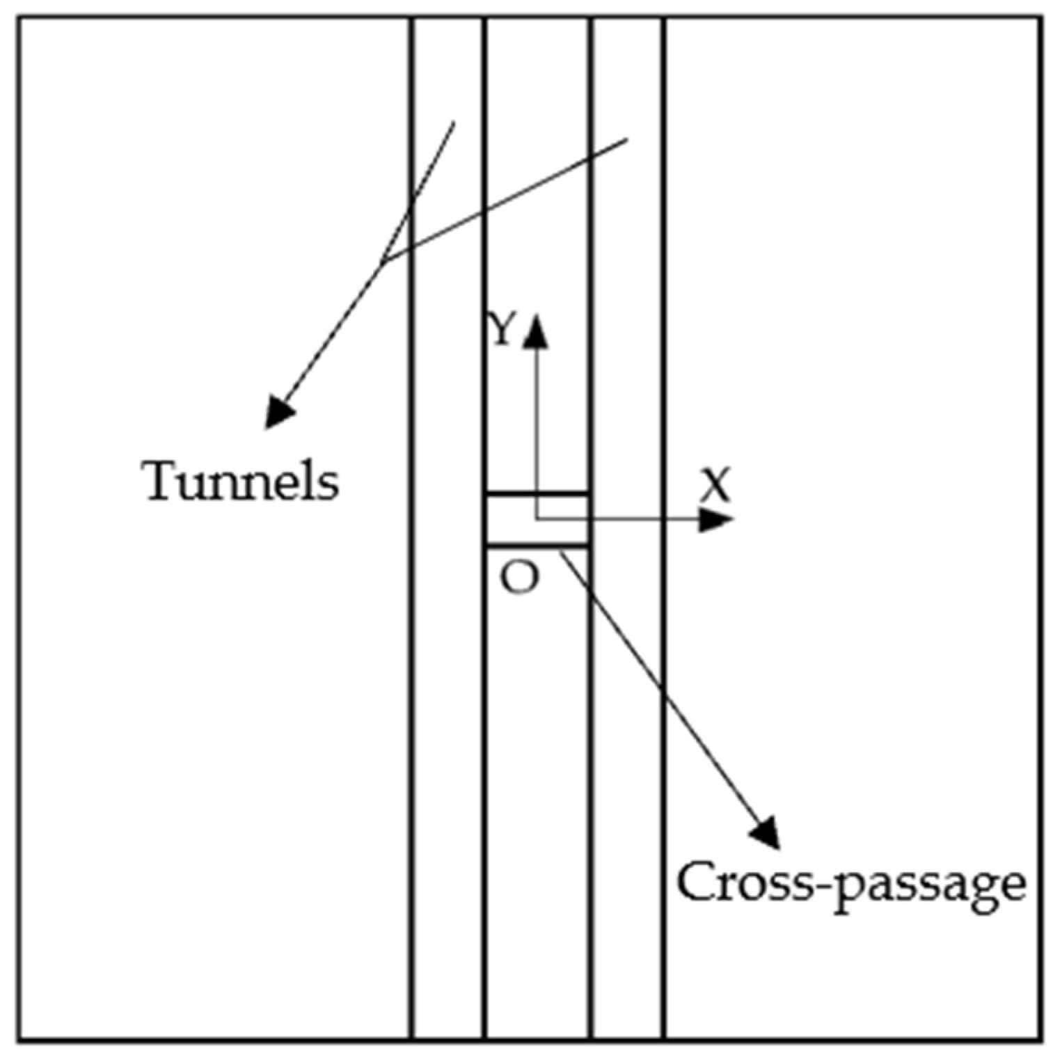
4.1. Model Geometry and Boundaries

The numerical model employed in this study, as shown in Figure 2, was built to simulate a typical application of the AGF method in the construction of a cross passage between two tunnels of an urban subway project. In this study, the focus is on the displacement of the ground surface; the groundwater dynamics, as suggested by Zheng [13], have little effect on it. Therefore, the effect of groundwater migration and interaction with the construction is not considered in the model. To reduce the model calculation time, only one layer of saturated clay was considered. The model geometry boundaries, as shown in Figure 2a, was set as 80 m × 80 m × 40 m, and the tunnels were located 20 m under the ground surface. As presented in Figure 2b, the two tunnels were 14 m away from each other with a 0.3 m thick shield tunnel segment. The arch-shaped cross passage, as illustrated in Figure 2c, was 4 m wide and high, and the liner within it was set as 0.1 m thick. When considering the differences in the thickness of the liners, the tunnel liners were simulated using volumetric elements, while the liners of the cross passage were modeled using shell elements. In addition, to examine the impact of the thickness of the freezing wall on ground surface deformation, five models with different freezing wall thicknesses, i.e., 1.0 m, 1.5 m, 2.0 m, 2.5 m, and 3.0 m, were developed.

For the mechanical boundaries, the top of the model was set as a free boundary, the bottom of the model was set as completely constrained, and the normal displacement of the four vertical faces of the model was set as constrained. For thermal conditions, the temperature field was initialized uniformly at 20 °C. Considering that the upper face of the model would be open to the external environment and exchange heat with it, the constant temperature boundary of 20 °C was fixed for all faces except for the top face, while the others were considered as adiabatic boundaries.

4.2. Simulation of Construction Procedures

The simulation of the construction procedures involved several activities, such as (1) stress initialization; (2) excavation of the tunnel and installation of the concrete liners; (3) artificial freezing of the surrounding soil of the cross passage; (4) excavation of the cross-passage and the installation of the liner; and (5) thawing of the freezing wall.

In phase (1), the initial stress was modeled by applying the gravity of 9.81 N/kg, with a coefficient of earth pressure at rest of 0.71. In phase (2), the excavation of the tunnel was simulated in 10 steps, with 8 m excavated in each step. While excavating the tunnel, the liners are installed simultaneously. In phase (3), the installation of the freezing pipes surrounding the cross passage was modeled, equivalent to the additional volumetric heat-absorbing source in the freezing wall. This volumetric source was added after the excavation of the tunnel, and it was removed before the excavation of the cross passage. In real-world engineering practices, the total power available for artificial freezing always has a limit, and thus, to control the variables of the freezing walls with different thicknesses, the total freezing power (in the unit of W) was set as the same. However, in FLAC3D, the valid input of freezing power is in unit volumetric form (in the unit of W/m³); therefore, as recommended by Zheng [13], the volumetric heat-absorbing source corresponding to a freezing wall with a thickness of 3 m was set as −25 W/m³, and the others were determined by keeping the total freezing power constant. In addition, the freezing period was determined by ensuring that the temperature throughout the freezing wall was below −10 °C. The source strength and freezing periods corresponding to the freezing walls with different thicknesses are summarized in

Table 1. Source strengths and freezing periods of different freezing wall thicknesses.

Thickness (m)	1.0	1.5	2.0	2.5	3.0
Source strength (W/m3)	−105	−64	−44	−32	−25
Freezing period (day)	18	26	36	48	60

. In phase (4), the excavation of the cross-passage was modeled in four steps.

4.3. Material Parameters

Material properties can be affected by temperature. When the temperature is below the freezing point, studies have shown that the physical parameters of reinforced concrete are insensitive to temperatures as low as −10 °C [21]. For soil, however, although properties such as friction angle are also less affected by temperature when below the freezing point [22], considerable research has shown that many properties of the soil, such as bulk modulus, shear modulus, cohesion, thermal conductivity, and specific heat capacity, are highly affected by the freezing and thawing process [23,24,25,26]. Moreover, these properties of the soil could be thought of as linear functions of temperature [27,28]. When the temperature falls into the range of freezing point to 20 °C, the physical properties of both soil and reinforced concrete are barely affected by the temperature change [25,29]. In addition, the properties of soils at the same temperature but under different processes (i.e., freezing or thawing process) have different values [13].

The data of the soil properties were retrieved from Zheng et al. [30] as shown in

Table 2. Mechanical properties of the materials.

Material	Temperature (°C)	Density (kg/m3)	Bulk Modulus (MPa)	Shear Modulus (MPa)	Constitutive Model	Friction Angle (°)	Cohesion (kPa)
Soil	20 (Original soil)	1880	16.67	7.69	Mohr–Coulomb	17 *	22
	−10	1880	106	57.9	Mohr–Coulomb	17 *	330
	20 (Thawed soil)	1880	40	18.46	Mohr–Coulomb	17 *	5.5
Liner of the tunnel	-	2500	2 × 104	1.5 × 104	Elastic	-	-
Liner of the cross passage	-	2400	1.56 × 104	1.17 × 104	Elastic	-	-

* When the temperature is above the freezing temperature, the thermal expansion coefficient of soils is positive and constant.

and

Table 3. Thermal properties of the materials.

Material	Temperature (°C)	Thermal Conductivity (W/m·°C)	Specific Heat Capacity (J/kg·°C)	Thermal Expansion Coefficient (°C−1)	Heave Rate (°C−1)	Thaw Settlement Rate (°C−1)
Soil	20	1.23	1040	1 × 10−5 *	-	-
	−10	1.38	1110	-	−9.64 × 10−4	−1.03 × 10−3
Liner of the tunnel	-	0.5	1000	1 × 10−5	-	-
Liner of the cross passage	-	- #	- #	1 × 10−5	-	-
Air in the tunnel	-	0.025	1000	-	-	-

* When the temperature is above the freezing temperature, the thermal expansion coefficient of soils is positive and constant. ^# Because the liners of the cross passage were simulated using shell element, these properties were currently not available for setting in FLAC3D.

. According to Zheng et al. [30], the freezing temperature of the soil was set as −0.56 °C. Following the discussion above, the properties of liners were treated as constant throughout the whole process, and the value of some properties, i.e., the bulk modulus, shear modulus, cohesion, thermal conductivity, and specific heat capacity of the soil under different processes, were determined by linear interpolation of the corresponding test results separately when the temperature of the soil was below the freezing point, but set as constant when the temperature was above the freezing point. The friction angle, on the other hand, was thought to be irrelevant to the changes in temperature within certain confining pressures, which is consistent with the experimental results obtained by Liu et al. [22]. In the numerical models, by utilizing the user-defined fish function in the FLAC3D, the properties of the soil were automatically adjusted with the change in temperature.

5. Results and Discussions

To present the results more clearly, the coordinates were constructed as illustrated in Figure 3 on the ground surface. The Y-axis is aligned with the longitudinal direction of the tunnel, while the X-axis is set as the transverse direction of the tunnel. In addition, the origin is right above the center of the cross passage.

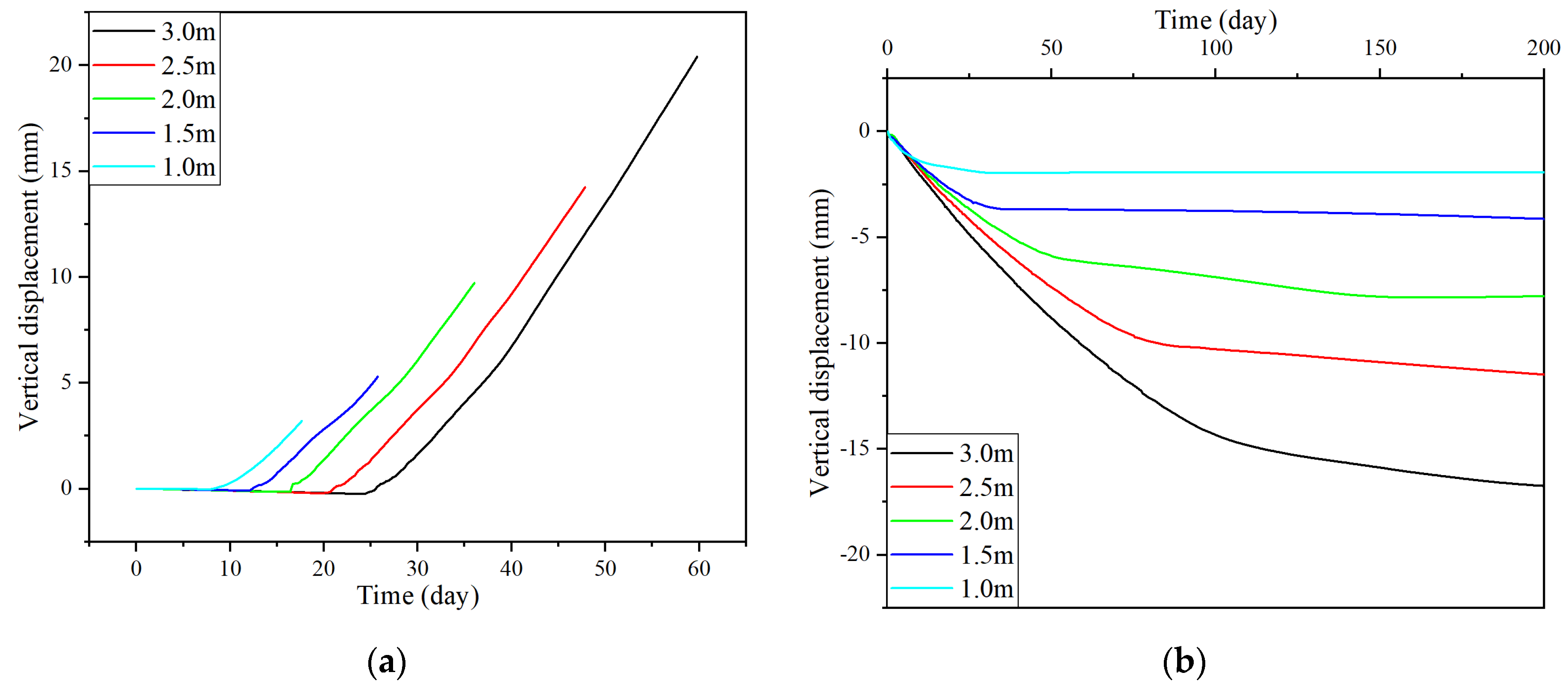
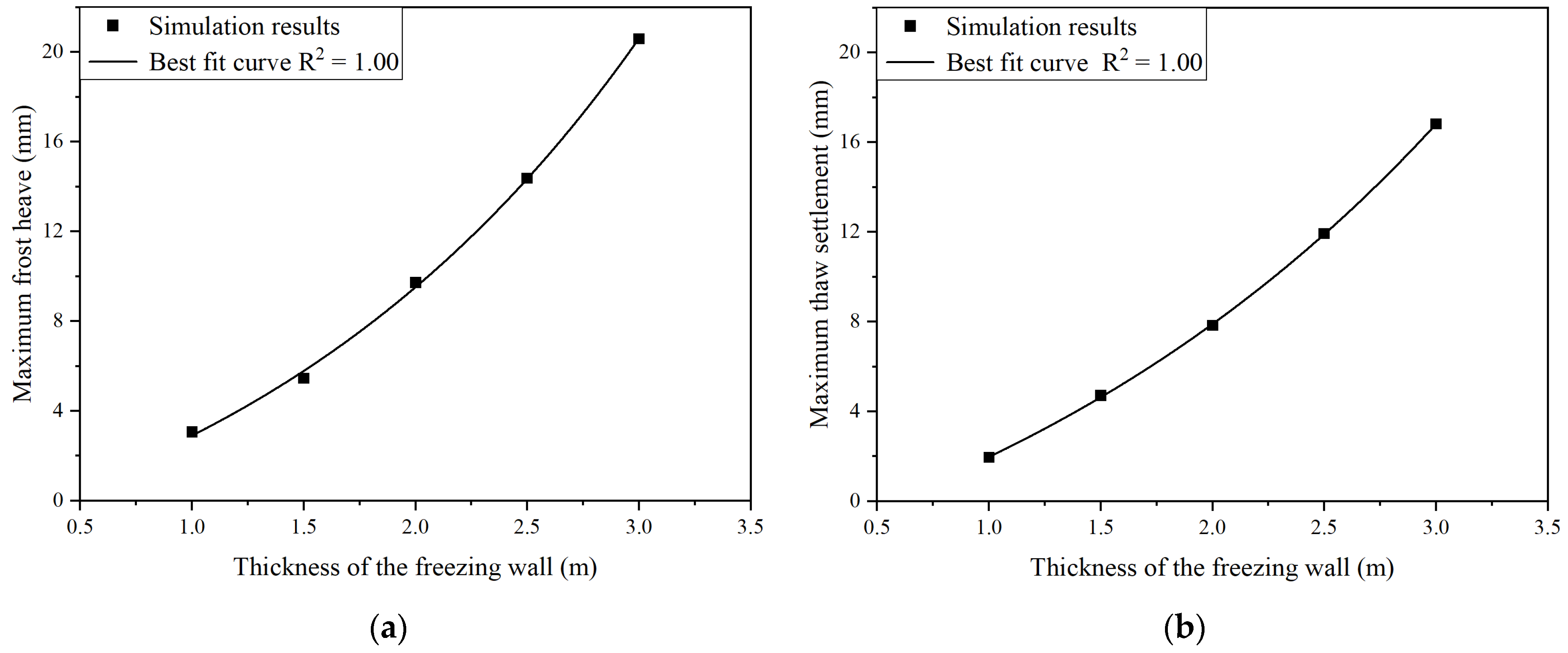
5.1. Development of Frost Heave and Thaw Settlement and How the Thickness of the Freezing Wall Affected Them

Figure 4 illustrates the frost heaves (the vertical displacements arising from the freezing process) and thaw settlements (the vertical displacements caused by the thawing process) at the origin O in Figure 3 induced by freezing walls of different thicknesses with respect to time. As illustrated in Figure 4a, there is a lag in the frost heave of the ground surface during the freezing process after the heat-absorbing source is added to the freezing wall. This lag corresponds to a slight settlement of the surface ground (the shrinkage stage), which is most likely caused by a small shrinkage in the soil before the temperature is below the freezing temperature of the soil. After passing the shrinkage stage, the frost heave begins to develop approximately linearly with respect to time (the fast-freezing stage). In addition, as shown in Figure 4b, the thawing process, the reversed process of the frost heave, shows ‘inverted’ curves compared with their counterparts of the frost heaving process. Similar to the the frost heave curve having a fast-freezing stage, the thaw settlement curve has a ‘fast-thawing stage’ just after the removal of the heat-absorbing source. Similar to the frost heave at the fast-freezing stage, the thaw settlement at the fast-thawing stage develops approximately linearly with a rather large slope. After the fast-thawing stage, the settlement becomes stable. These results are similar to that reported by Zheng et al. [2].

An increase in the thickness of the freezing wall in the freezing process, as illustrated in Figure 5, can prolong the period of freezing. In addition, the shrinkage period of the frost heave extends linearly with an increase in the thickness of the freezing wall, while the fast-freezing stage lengthens faster and nonlinearly. In the thawing process, as shown in Figure 6, with an increase in the thickness of the freezing wall, the fast-thawing stage also extends, and the effect on it is much more apparent than that shown on the fast-freezing stage.

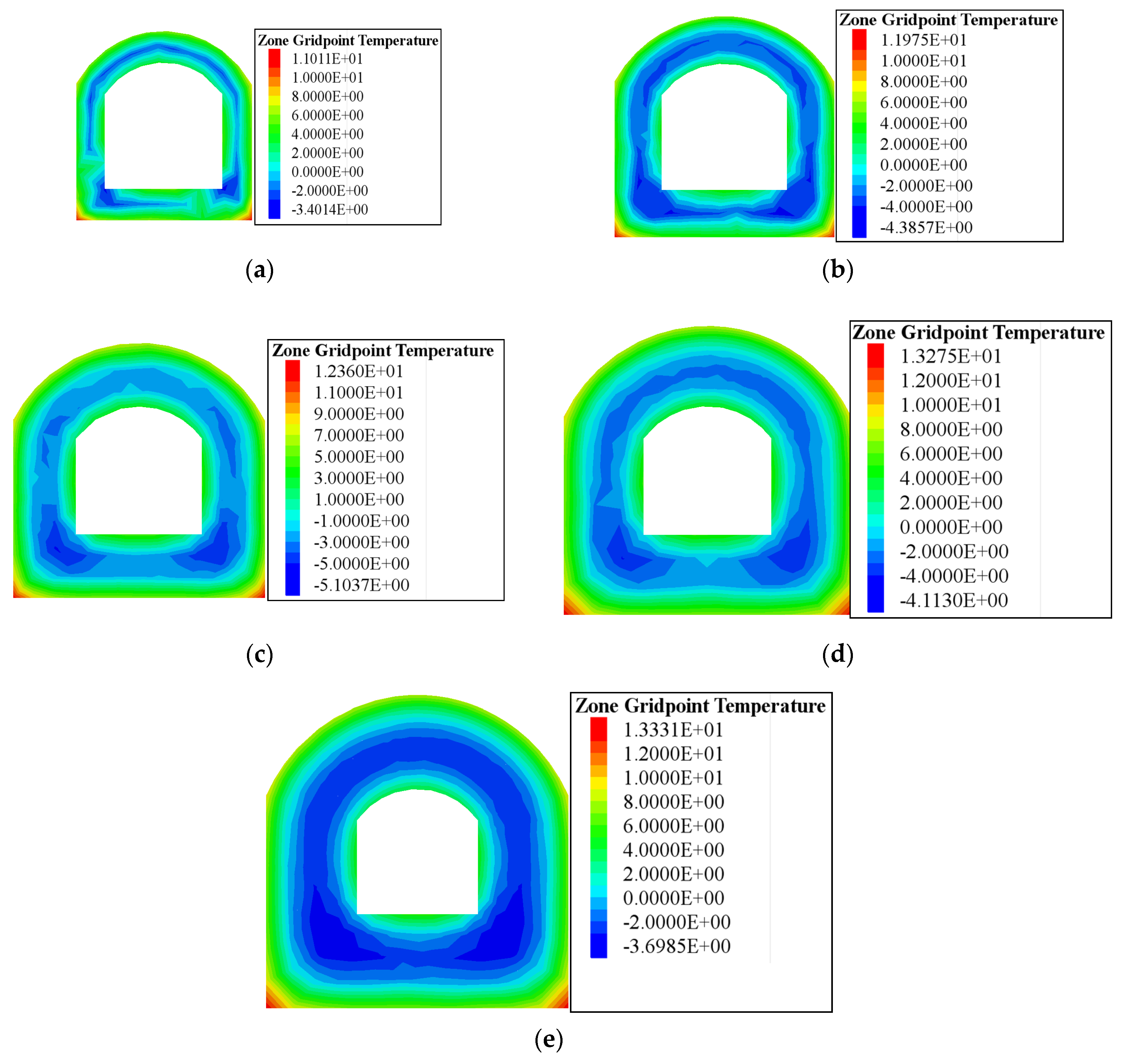
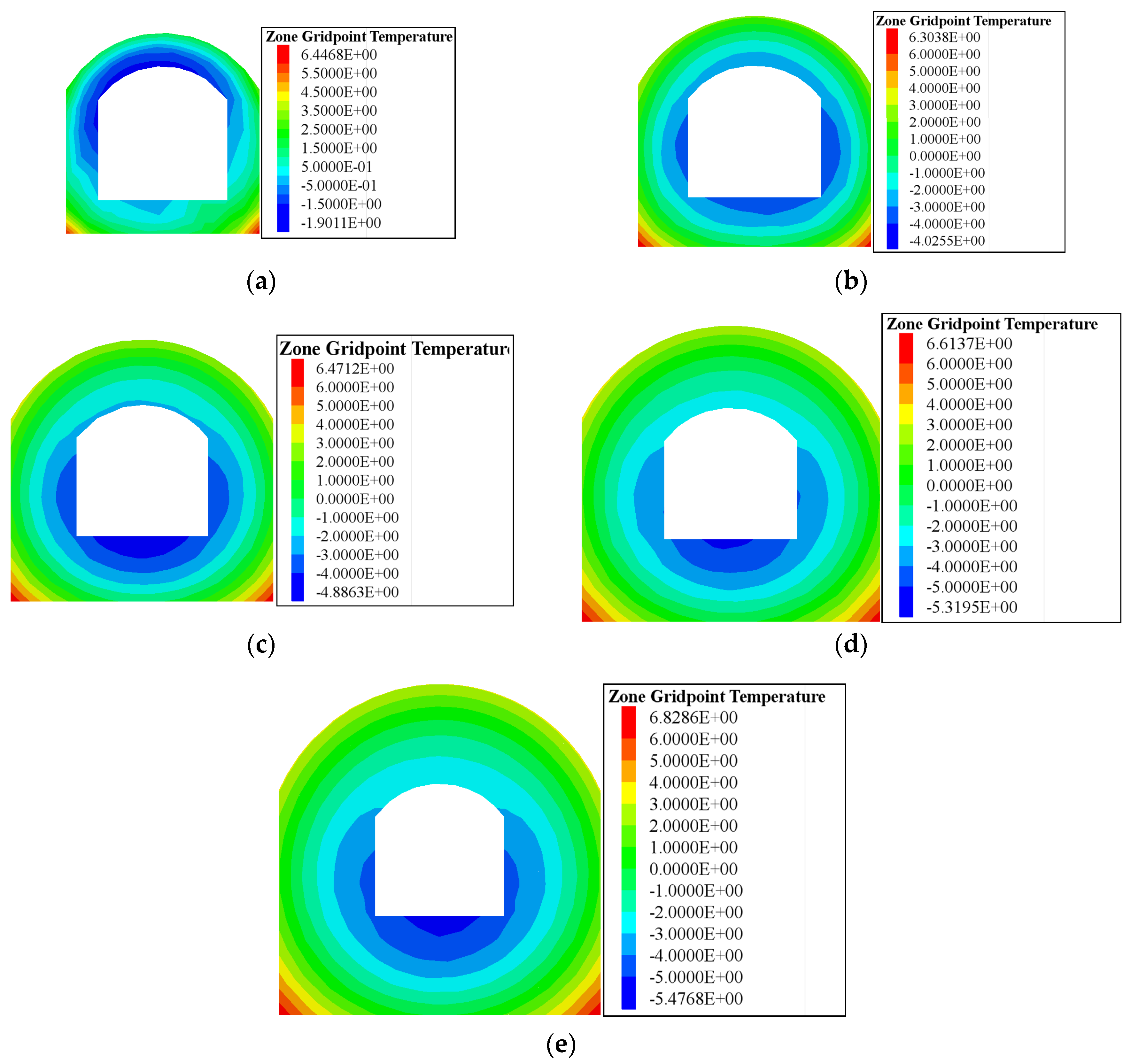
5.2. Temperature Distribution within the Freezing Wall at Two Characteristic Time Points

As mentioned in the Section 1, problems concerning temperature distribution within freezing walls have long been of great interest. In this study, the temperature distribution within the freezing wall at two characteristic time points, i.e., the starting point of the fast-freezing stage and the finishing point of the fast-thawing stage, were investigated. These two points were selected to shed light on the identification and explanation of the beginning of the fast-freezing stage and the end of the fast-thawing stage with temperature distribution. The distribution results are presented in Figure 7 and Figure 8. Figure 7 illustrates the temperature distribution within freezing walls of different thicknesses at the cross-section of the Y-axis right before the fast-freezing stage. Before entering the fast-freezing stage, the temperature of the area right around the cross passage would already have been below freezing temperature. This may be traced to the shrinkage of the unfrozen soil due to the drop in the temperature. The shrinkage of the soil cancels part of the frost heave. Therefore, part of the soil froze ahead of the commencement of the frost heave of the ground surface. In addition, as shown in Figure 7, the lowest temperature within the freezing wall at this time point first drops and then increases with an increase in the thickness of the freezing wall. Figure 8 demonstrates the temperature distribution within freezing walls of different thicknesses at the cross-section of the Y-axis right after the fast-thawing stage. Like its counterpart in the freezing process, when achieving a stable settlement, the temperature of some areas in the middle of the freezing wall would still have been below freezing temperature. There are several potential explanations for this. There was only a very thin layer of frozen soil within the freezing wall, and most of the soil was in a thawed state. Therefore, the displacement arising from thawing would not contribute too much to the entire thawing settlement. In addition to this, when the temperature rises during the thawing process, the unfrozen soil expands, and this also counteracts the thaw settlement of the ground surface. Therefore, part of the soil remains frozen when the settlement is about to become stable. Figure 8 also shows that the lowest temperature within the freezing wall at this time point drops with an increase in the thickness of the freezing wall in a gradual, gentle way. Apart from this, it can be seen that with an increase in the thickness of the freezing wall, the center of the temperature contour moves downward. This may arise from the setting of the temperature thermal boundary at the top of the model. The temperature at the top of the model is fixed and can be thought of as a heat source which transfers the heat downward to the freezing wall, where the temperature is much lower than the surrounding soil. This heat transfer movement makes the temperature of the upper side of the cross passage higher than that of the lower side. This effect might be more apparent as the prolongation of the fast-thawing stage with an increase in the thickness of the freezing wall.

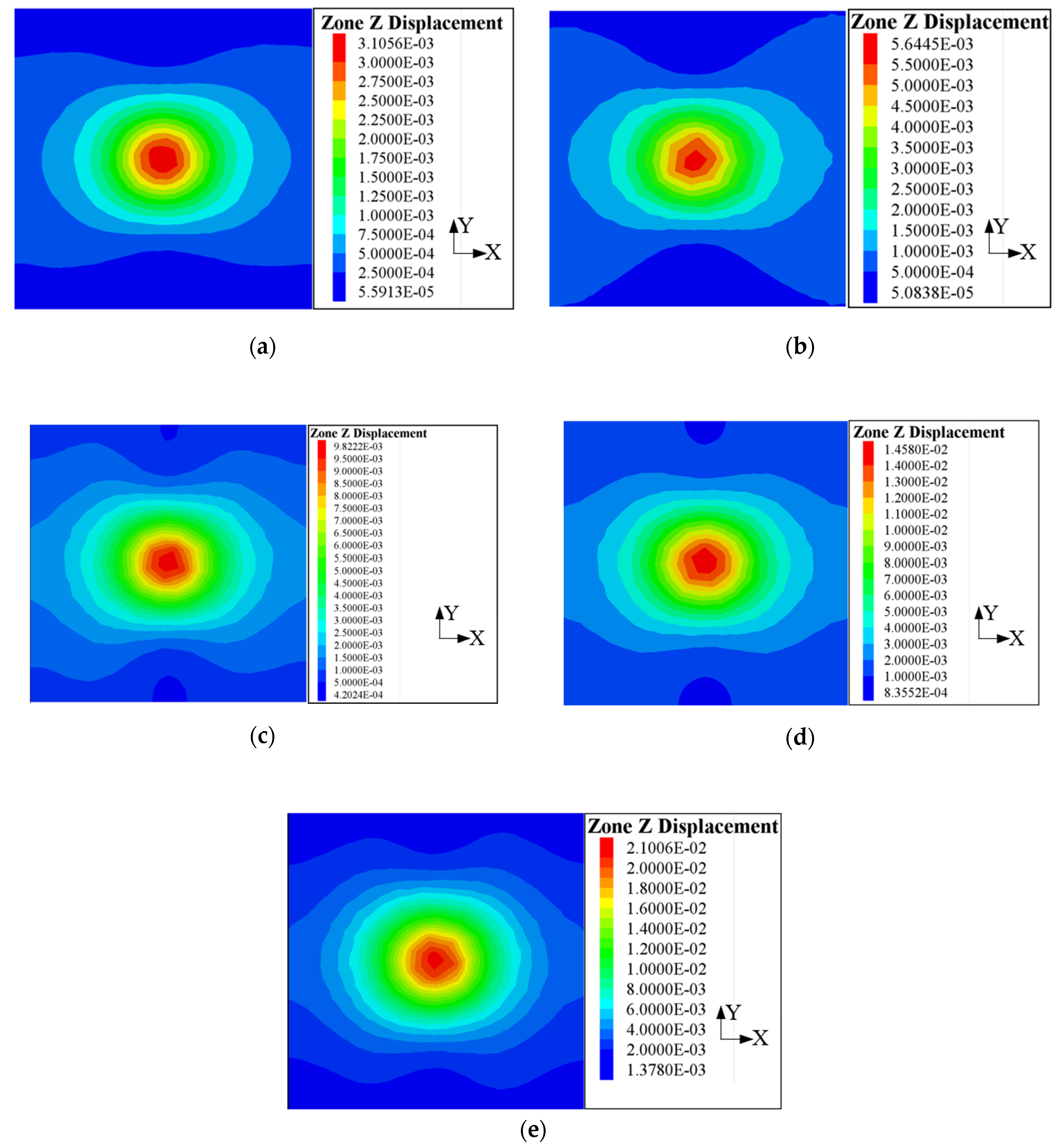
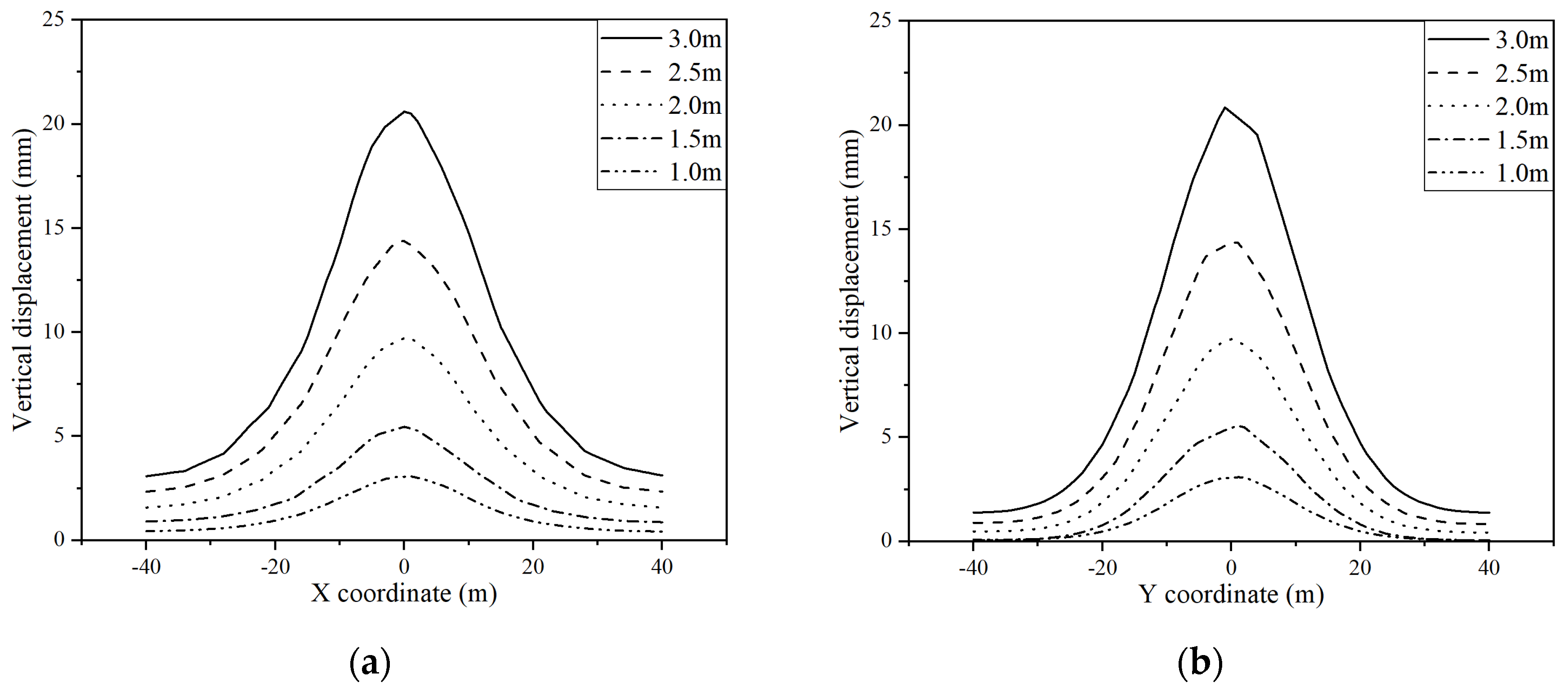
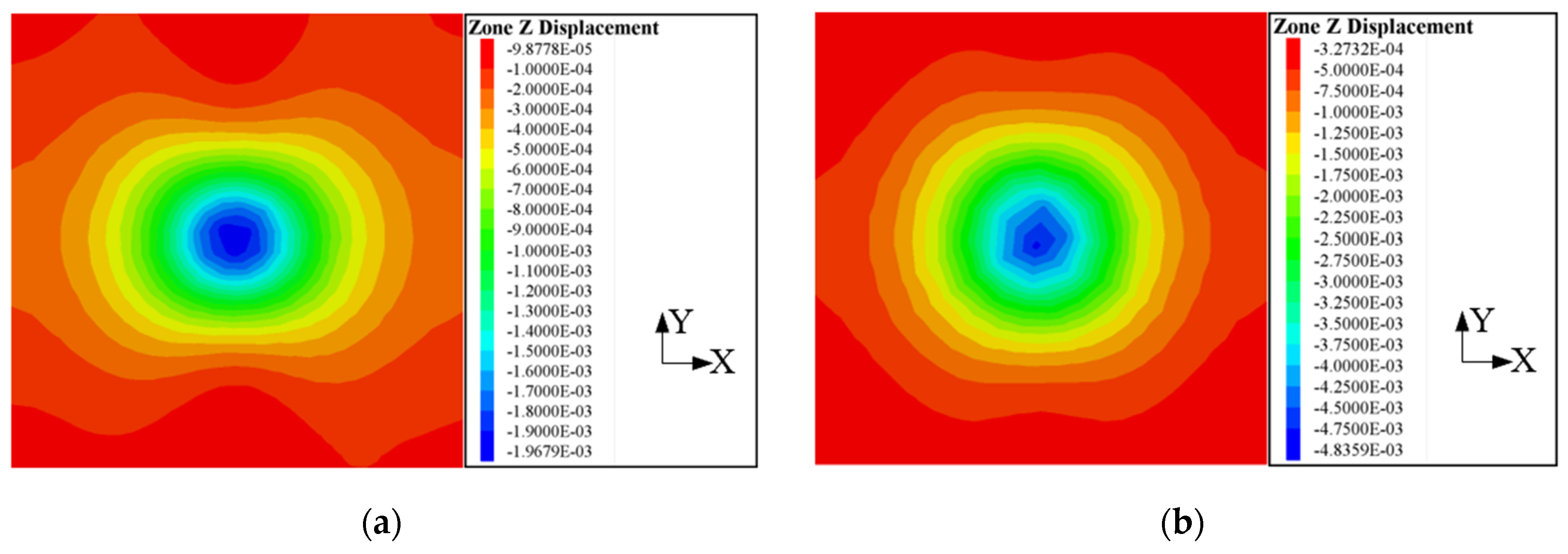
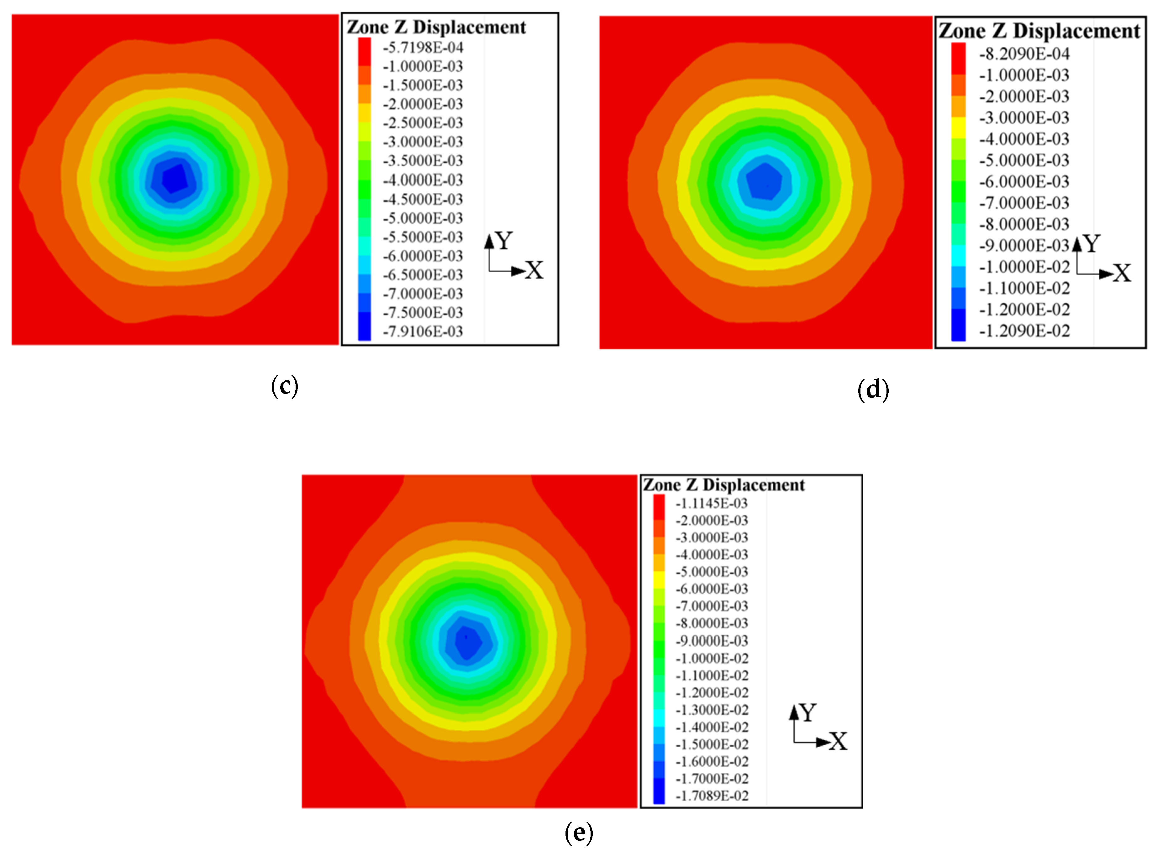
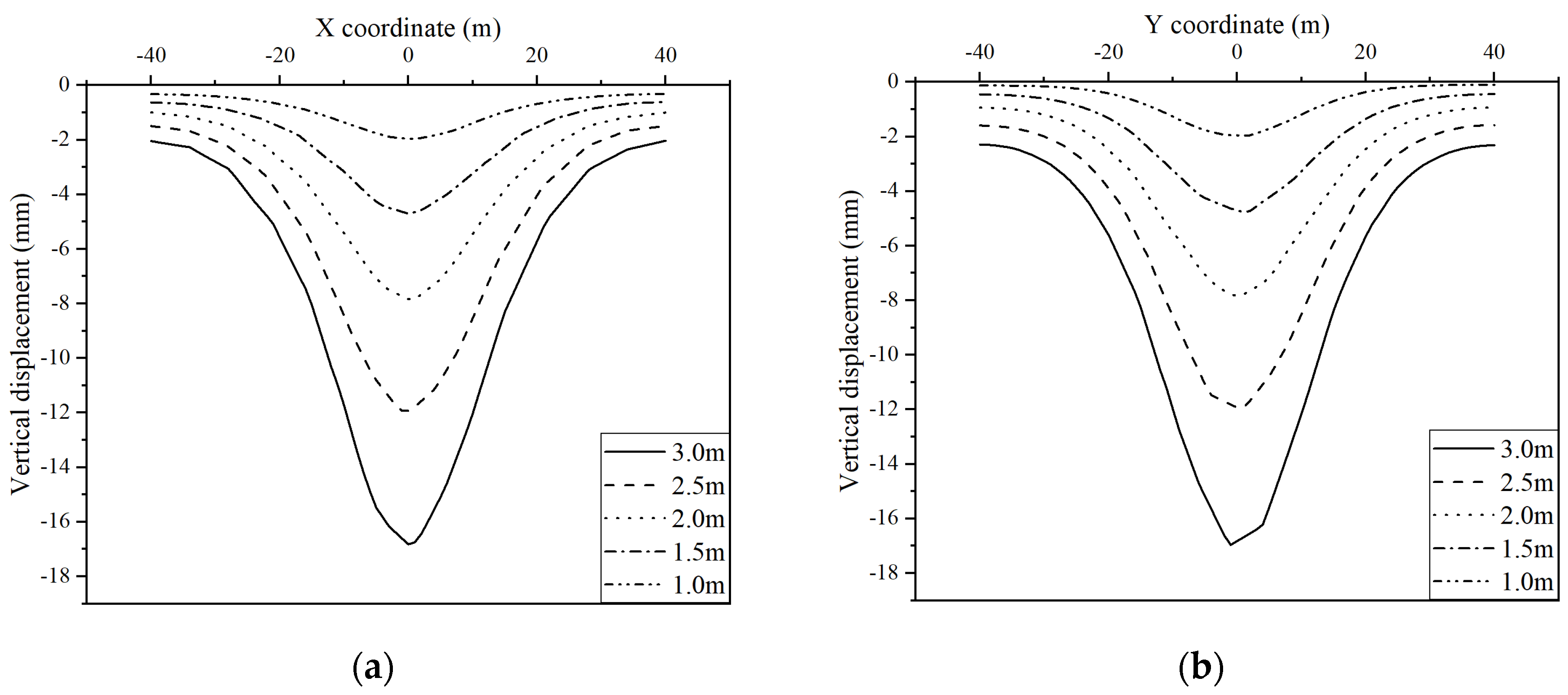
5.3. Spatial Distribution of Frost Heave and Thaw Settlement and How the Thickness of the Freezing Wall Affected It

Figure 9 and Figure 10 reveal that the frost heave distribution along the X-axis is wider than that along the Y-axis. This reveals that the frost heave has a gentler variation in the transverse direction of the tunnel, yet a more marked variation in the longitudinal direction of the tunnel. On the contrary, as illustrated by Figure 11 and Figure 12, except for that corresponding to the freezing wall with a thickness of 1 m, thaw settlement distribution along the X-axis has a similar size to that along the Y-axis, which represents that the fluctuation of the thaw settlement along the longitudinal direction of the tunnel is approximately as large as that along the transverse direction of the tunnel. Furthermore, Figure 11 conveys that the settlement is distributed uniformly among different directions. In addition, as presented by Figure 10 and Figure 12, with the increase in the thickness of the freezing wall, the frost heave and the thaw settlement grow accordingly. In addition, to qualify the effects of the thickness of the freezing wall on the maximum ground surface displacements, an attempt was made to fit the simulation results into mathematical equations. It was found that the exponential equation (Equation (11)) can best represent the trends with respect to the thickness of the freezing wall, which consequently implies that the increase in the thickness of the freezing wall might give rise to an exponential growth in the displacements of the ground surface. The fitting parameters are summarized in

Table 4. Fitting results of the maximum vertical displacements.

	Fitting Parameters			R2
	y0	A	k
Maximum frost heave	−6.83	5.80	0.52	1.00
Maximum thaw settlement	−9.70	7.75	0.41	1.00

, and the fitting results are shown in Figure 13.

$$y=y_0+A{e}^{kx}$$

(11)

where y₀, A, and k are the fitting parameters.

To evaluate the displacement distribution of frost heave and thaw settlement quantitively, the absolute values of the displacement data of the frost heave and thaw settlement gained from the numerical simulation were fitted to the amplitude version of the Gaussian peak function in the form of Equation (12). The results are summarized in

Table 5. The fitting results of the displacement data of the frost heave and thaw settlement.

Thickness of the Freezing Wall (m)	Displacement Type	Direction of the Cross-Section	y0	xc	w	A	y0 + A	R2
1.0 m	Frost heave	X-axis	0.48	−0.03	10.42	2.52	3.00	1.00
		Y-axis	0.08	0.05	9.81	2.97	3.05	1.00
1.5 m		X-axis	0.98	−0.15	10.32	4.29	5.27	1.00
		Y-axis	0.06	0.03	9.99	5.34	5.40	1.00
2.0 m		X-axis	1.75	0.03	10.92	7.71	9.47	1.00
		Y-axis	0.48	−0.01	10.16	9.09	9.57	1.00
2.5 m		X-axis	2.51	0.11	11.37	11.54	14.05	1.00
		Y-axis	0.91	−0.15	10.31	13.34	14.25	1.00
3.0 m		X-axis	3.37	0.15	11.30	16.82	20.19	1.00
		Y-axis	1.49	0.09	10.48	18.91	20.40	1.00
1.0 m	Thaw settlement	X-axis	0.35	0.11	11.14	1.57	1.92	1.00
		Y-axis	0.12	−0.35	10.09	1.83	1.95	1.00
1.5 m		X-axis	0.69	0.04	11.19	3.88	4.57	1.00
		Y-axis	0.48	0.06	11.19	4.17	4.65	1.00
2.0 m		X-axis	1.12	0.02	11.51	6.51	7.64	1.00
		Y-axis	0.97	0.00	11.40	6.72	7.70	1.00
2.5 m		X-axis	1.61	0.10	11.69	10.08	11.69	1.00
		Y-axis	1.63	−0.07	11.43	10.19	11.82	1.00
3.0 m		X-axis	2.24	0.08	11.64	14.24	16.48	1.00
		Y-axis	2.38	0.11	11.50	14.29	16.68	1.00

. As illustrated in Table 5, the parameter w, governing the width of the distribution curve, is larger for the curves of the X-axis than those of the Y-axis, which indicates that the curves along the X-axis are wider than those along the X-axis. This may stem from the geometrical shape of the freezing wall, which is longer in the direction of the X-axis than the Y-axis. The longer side might give rise to a wider settlement, while the shorter side causes a narrower one. However, the difference between them is rather sharp in the curves of frost heave, yet relatively minor in those of thaw settlement, which is consistent with what is shown in Figure 9 and Figure 10. It is also noteworthy that the values of the w of the thaw settlement curves are larger than those of the frost heave curves, which indicates that the thaw settlement curves are generally gentler than the frost heave curves. In addition, the value of w slightly grows with an increase in the thickness of the freezing wall, which implies that the displacement distribution of the frost heave and thaw settlement becomes wider with an increase in the thickness of the freezing wall.

For the maximum absolute values of the displacement curve, which are indicated by y₀ + A, although the thaw settlement rate is slightly larger than the frost heave rate, those of the frost heave are larger than those corresponding to the thaw settlement. This may be attributed to the excavation of the cross passage and the installation of the liners. When freezing the surrounding soil of the cross passage, part of the soil within the cross passage area will also freeze. However, when excavating the cross passage, this part of the soil will be removed, which will reduce the volume of the soil which has the potential to settle, along with the restriction of the settlement imposed by the liners. These two factors might work together to lead to a smaller displacement of the thawing process.

$$y=y_0+A{e}^{-\frac{{(x-x_c)}^2}{2w^2}}$$

(12)

where A is the parameter related to the amplitude of the curve, where a larger A will result in a higher peak; x_c determines the location of the center of the curve; w has an impact on the width of the curve, where a greater w will yield a wider curve; and y₀ is the parameter indicating the base of the curve, where a larger y₀ will yield a higher base.

6. Conclusions

In this paper, the frost heave and thaw settlement induced by freezing walls in the AGF method, which are inadequately investigated in the current literature, are systematically examined by a set of state-of-the-art numerical models built by FLAC3D with the data retrieved from the literature. Similar to the results reported by Zheng et al. [2], for the characteristics of the freezing and thawing processes, our results show that a shrinkage stage occurs before entering the linear fast-freezing stage and the settlement becomes stable after a linear fast settlement during the thaw settlement. For temperature distribution within a freezing wall, it is found that the temperature of a certain area within the freezing wall is below freezing temperature prior to the fast-freezing stage and after the fast-thawing stage. For ground displacement, the results indicate that during the frost heave process, the displacement curve along the transverse direction of the tunnel is wider than that along the longitudinal direction of the tunnel, while that of the thaw settlement is comparatively uniform in different directions.

In terms of the effects of the thickness of the freezing wall on the freezing and thawing characteristics, it is observed that (1) the increase in the thickness of the freezing wall gives rise to the extension of the freezing process and the fast-thawing stage; (2) similar to that pointed out by Zheng [13], the frost heave and thaw settlement of the ground surface might increase exponentially with growth in the thickness of the freezing wall, which can be informative when it comes to the determination of the thickness of the freezing wall; and (3) the thickness of the freezing wall is also a contributory factor to a more gentle displacement distribution of the surface ground.

This study provided insights into the ground displacements during the freezing and thawing processes of artificial freezing methods in the construction of subway cross passages. However, in this study, the groundwater movement during freezing and thawing process was not considered. More research is needed to investigate the interaction of groundwater dynamics with the freezing and thawing processes.

References

1. Lu, X.; Chen, X.; Chen, X. Risk Prevention and Control of Artificial Ground Freezing (AGF). Chin. J. Geotech. Eng. 2021, 43, 2308–2314. [Google Scholar]
2. Zheng, L.; Gao, Y.; Zhou, Y.; Liu, T.; Tian, S. A Practical Method for Predicting Ground Surface Deformation Induced by the Artificial Ground Freezing Method. Comput. Geotech. 2021, 130, 103925. [Google Scholar] [CrossRef]
3. Domke, O. Über Die Beanspruchung Der Frostmauer Beim Schachtabteufen Nach Dem Gefrierverfahren. Glückauf 1915, 51, 1129–1135. [Google Scholar]
4. Zhou, X.; Jiang, G.; Li, F.; Gao, W.; Han, Y.; Wu, T.; Ma, W. Comprehensive Review of Artificial Ground Freezing Applications to Urban Tunnel and Underground Space Engineering in China in the Last 20 Years. J. Cold Reg. Eng. 2022, 36, 04022002. [Google Scholar] [CrossRef]
5. Yue, F.; Qiu, P.; Yang, G.; Shi, R. Design and Practice of Freezing Method Applied to Connected Aisle in Tunnel under Complex Conditions. Chin. J. Geotech. Eng. 2006, 28, 660–663. [Google Scholar]
6. Fang, L.; Li, F.; Cui, H.; Ding, H. Research on Freezing Wall Thickness Design of Metro Cross Passage Based on Structural Mechanics Method. Urban Mass. Transit. 2020, 23, 117–121. [Google Scholar]
7. Liu, Z. Study on the Thickness Design of the Freezing Wall of the Subway Liaison Channel in the Water Rich Gravel Stratum; Xi’an University of Science and Technology: Xi’an, China, 2018. [Google Scholar]
8. Zhou, F.; Zhou, P.; Li, J.; Ge, T.; Lin, J.; Wang, Z. Key Parameters Design Method of AGF Method for Metro Connecting Passage in Water-Rich Coastal Area. KSCE J. Civ. Eng. 2022, 26, 5301–5317. [Google Scholar] [CrossRef]
9. Yan, S.; Li, J.; Sun, L.; Wu, K. Study on Design and Calculating Methods of Artificial Freezing Curtain on Metro Connected Passage-Way Project. Site Investig. Sci. Technol. 2014, 2014, 5–10. [Google Scholar]
10. Tang, Y.; Xiao, S.; Zhou, J. Deformation Prediction and Deformation Characteristics of Multilayers of Mucky Clay under Artificial Freezing Condition. KSCE J. Civ. Eng. 2019, 23, 1064–1076. [Google Scholar] [CrossRef]
11. Li, J.; Li, J.; Cai, Y.; Wu, D.; Guo, C.; Zhao, W.; Tang, K.; Liu, Y. Application of Artificial Freezing Method in Deformation Control of Subway Tunnel. Adv. Mater. Sci. Eng. 2022, 2022, 3251318. [Google Scholar] [CrossRef]
12. Zhou, J.; Tang, Y. Practical Model of Deformation Prediction in Soft Clay after Artificial Ground Freezing under Subway Low-Level Cyclic Loading. Tunn. Undergr. Space Technol. 2018, 76, 30–42. [Google Scholar] [CrossRef]
13. Zheng, L. Research on Optimization Method and Engineering Application of Frozen Wall Thickness for Cross-Passage in Urban Rail Transit; University of Science and Technology Beijing: Beijing, China, 2021. [Google Scholar]
14. Cai, H.; Peng, L.; Zheng, T. Prediction Method of Surface Frost Heave Based on Stochastic Medium Theory in Tunnel Freezing Period. J. Cent. South Univ. 2014, 45, 4251–4257. [Google Scholar]
15. Cai, H.; Liu, Z.; Li, S.; Zheng, T. Improved Analytical Prediction of Ground Frost Heave during Tunnel Construction Using Artificial Ground Freezing Technique. Tunn. Undergr. Space Technol. 2019, 92, 103050. [Google Scholar] [CrossRef]
16. Zhang, Z.; He, C. Study on Construction of Cross Connection of Shield Tunnel and Connecting Aisle by Freezing Method. Chin. J. Rock Mech. Eng. 2005, 24, 3211–3217. [Google Scholar]
17. Fu, Y.; Hu, J.; Wu, Y. Finite Element Study on Temperature Field of Subway Connection Aisle Construction via Artificial Ground Freezing Method. Cold Reg. Sci. Technol. 2021, 189, 103327. [Google Scholar] [CrossRef]
18. Huang, S.; Guo, Y.; Liu, Y.; Ke, L.; Liu, G.; Chen, C. Study on the Influence of Water Flow on Temperature around Freeze Pipes and Its Distribution Optimization during Artificial Ground Freezing. Appl. Therm. Eng. 2018, 135, 435–445. [Google Scholar] [CrossRef]
19. Zhang, S.; Zhou, X.; Zhang, J.; Sun, T.; Ma, W.; Liu, Y.; Yang, N. A Case Study of Energy-Saving and Frost Heave Control Scheme in Artificial Ground Freezing Project. Geofluids 2022, 2022, 1004735. [Google Scholar] [CrossRef]
20. Cai, H.; Li, S.; Liang, Y.; Yao, Z.; Cheng, H. Model Test and Numerical Simulation of Frost Heave during Twin-Tunnel Construction Using Artificial Ground-Freezing Technique. Comput. Geotech. 2019, 115, 103155. [Google Scholar] [CrossRef]
21. Lee, G.C.; Shih, T.S.; Chang, K.-C. Mechanical Properties of Concrete at Low Temperature. J. Cold Reg. Eng. 1988, 2, 13–24. [Google Scholar] [CrossRef]
22. Liu, X.; Liu, E.; Zhang, D.; Zhang, G.; Song, B. Study on Strength Criterion for Frozen Soil. Cold Reg. Sci. Technol. 2019, 161, 1–20. [Google Scholar] [CrossRef]
23. Liu, J.; Chang, D.; Yu, Q. Influence of Freeze-Thaw Cycles on Mechanical Properties of a Silty Sand. Eng. Geol. 2016, 210, 23–32. [Google Scholar] [CrossRef]
24. Wang, D.; Ma, W.; Niu, Y.; Chang, X.; Wen, Z. Effects of Cyclic Freezing and Thawing on Mechanical Properties of Qinghai–Tibet Clay. Cold Reg. Sci. Technol. 2007, 48, 34–43. [Google Scholar] [CrossRef]
25. Özgan, E.; Serin, S.; Ertürk, S.; Vural, I. Effects of Freezing and Thawing Cycles on the Engineering Properties of Soils. Soil Mech. Found. Eng. 2015, 52, 95–99. [Google Scholar] [CrossRef]
26. Kok, H.; McCool, D.K. CRREL Special Report 90-1; CRREL Special and Products: Hanover, NH, USA, 1990; pp. 70–76. [Google Scholar]
27. Christ, M.; Kim, Y.-C.; Park, J.-B. The Influence of Temperature and Cycles on Acoustic and Mechanical Properties of Frozen Soils. KSCE J. Civ. Eng. 2009, 13, 153–159. [Google Scholar] [CrossRef]
28. Wang, D.; Zhu, Y.; Ma, W.; Niu, Y. Application of Ultrasonic Technology for Physical–Mechanical Properties of Frozen Soils. Cold Reg. Sci. Technol. 2006, 44, 12–19. [Google Scholar] [CrossRef]
29. Shoukry, S.N.; William, G.W.; Downie, B.; Riad, M.Y. Effect of Moisture and Temperature on the Mechanical Properties of Concrete. Constr. Build. Mater. 2011, 25, 688–696. [Google Scholar] [CrossRef]
30. Zheng, L.; Gao, Y.; Zhou, Y.; Tian, S. Research on Surface Frost Heave and Thaw Settlement Law and Optimization of Frozen Wall Thickness in Shallow Tunnel Using Freezing Method. Rock Soil Mech. 2020, 41, 10. [Google Scholar]
Figure 1. The schematic diagram of the tetrahedron element used in FLAC3D.
Applsci 14 04220 g001
Figure 2. Dimensions of the model. (a) Dimensions of the overall model; (b) dimensions of the tunnel; (c) dimensions of the cross-passage.
Applsci 14 04220 g002
Figure 3. The schematic diagram of the coordinate used in the presentation of the results.
Applsci 14 04220 g003
Figure 4. Development of the frost heave and thaw settlement induced by the freezing walls with different thicknesses. (a) Development of the frost heave; (b) development of the thaw settlement.
Applsci 14 04220 g004
Figure 5. Changes in the time corresponding to the shrinkage stage, the fast-freezing stage, and the total freezing process with an increase in the thickness of the freezing wall.
Applsci 14 04220 g005
Figure 6. Changes in the time corresponding to the fast-freezing stage and the fast-thawing stage with an increase in the thickness of the freezing wall.
Applsci 14 04220 g006
Figure 7. The temperature distribution within freezing walls of different thicknesses at the cross-section of the Y-axis at the starting point of the fast-freezing stage: (a) 1.0 m on the 8th day; (b) 1.5 m on the 12th day; (c) 2.0 m on the 16th day; (d) 2.5 m on the 20th day; (e) 3.0 m on the 25th day.
Applsci 14 04220 g007
Figure 8. The temperature distribution within freezing walls of different thicknesses at the cross-section of the Y-axis at the finishing point of the fast-thawing stage: (a) 1.0 m on the 12th day; (b) 1.5 m on the 26th day; (c) 2.0 m on the 52nd day; (d) 2.5 m on the 75th day; (e) 3.0 m on the 100th day.
Applsci 14 04220 g008
Figure 9. The displacement contours of the frost heave induced by freezing walls of different thicknesses: (a) 1.0 m; (b) 1.5 m; (c) 2.0 m; (d) 2.5 m; (e) 3.0 m.
Applsci 14 04220 g009
Figure 10. The displacement distribution curves of the frost heave of the ground surface (a) along the X-axis and (b) along the Y-axis.
Applsci 14 04220 g010
Figure 11. The displacement contours of the thaw settlement induced by freezing walls of different thicknesses: (a) 1.0 m; (b) 1.5 m; (c) 2.0 m; (d) 2.5 m; (e) 3.0 m.
Applsci 14 04220 g011aApplsci 14 04220 g011b
Figure 12. The displacement distribution curves of the thaw settlement of the ground surface (a) along the X-axis and (b) along the Y-axis.
Applsci 14 04220 g012
Figure 13. The variation in the maximum vertical displacements with respect to freezing wall thickness: (a) frost heave; (b) thaw settlement.
Applsci 14 04220 g013