Analytical Solution for Seismic Stability of 3D Rock Slope Reinforced with Prestressed Anchor Cables

Abstract

Currently, the study of analytical solutions for the seismic stability of slopes under anchorage conditions is one of the hottest subjects in engineering. In this paper, an analytical solution for the seismic safety of the three-dimensional (3D) two-stage rock slope reinforced with prestressed anchor cables governed by the nonlinear Hoek–Brown criterion was deduced, in which the analyses of seismicity were performed by the latest modified pseudo-dynamic method. This method supplements the consideration of the damping effect of the rock medium on seismic waves, which is more in line with the real seismic situation. A mathematical geometric model was developed for calculating the external forces work and internal energy dissipation acting on 3D rotating rock masses reinforced with prestressed anchor cables, in which the seismic work rate was calculated using a new layer-by-layer superposition summation method. The analytical solution of the safety factor could be collated as an explicit function of several variables, and then, the optimal value was obtained by the Particle Swarm Optimization (PSO) algorithm. To corroborate the accuracy of new analytical solutions, the results were contrasted with those of the pertinent literature. The results of the two comparisons were very close. Ultimately, the sensitivity analyses and coupling effects of seismic pseudo-dynamic factors and prestressing anchorage factors were carried out. It was found that even small seismic intensities had a large effect on the stability of rock slopes with developed joints. Increasing the number of steps and prestressing anchors can effectively improve the stability of rock slopes under seismic effects. The conclusions have significant implications for the anchorage design of the 3D two-stage rock slope as seismic events occur.

1. Introduction

The analytical computation for rock slope stability disturbed by large seismicity has traditionally been one of the challenges in the field of engineering. For slopes with poor-quality lithological media, prestressed anchor cables are commonly employed as a means of reinforcement [1,2,3,4]. It can provide the resistance force acting on the structure to bear the external load and creates a compressive stress zone within the anchored rock layer, which allows the weak rock slope to resist heavy seismic effects [5,6]. Moreover, there is a considerable amount of research on two-dimensional (2D) slopes reinforced with prestressed anchor cables in the previous literature, while slopes are indeed frequently in the three-dimensional (3D) status, which has received little attention [7,8]. Currently, the safety assessment approaches of the 3D slope are primarily of the following three types: (1) limit equilibrium (LE), (2) limit analysis (LA), and (3) finite element (FE). Among these, the LA of plasticity ignores the elastic–plastic process during rock mass failure and directly analyzes the limit state of 3D slopes [9]. Since LA can readily obtain the exact analytical solution [10,11] as well as avoid the irrational assumptions of LE and the time-consuming computations of FE [12], this method is utilized in this paper.

Building the kinematically admissible failure mechanism is the main difficulty with utilizing LA to solve the stability solution, and there is a wealth of literature in this area of study [13,14,15]. For the first time, a 3D sliding mechanism composed of numerous logarithmic spirals was created in order to investigate the 3D stability of vertically tangential slopes at different angles [16]. A 3D integral sliding mechanism was constructed, and the effect of slope top foundation load on the overall and local stability of the slope was examined using this sliding mechanism [17]. Considering the volume deformation of sliding bodies for slopes, a horn-shaped rotating sliding mechanism for 3D stability analysis of slopes with soil or rock was proposed [18], and it was adopted in this paper.

For rock media, the Hoek–Brown (H-B) yield criterion is one of the most frequently employed strength criteria [19]; it was proposed based on triaxial tests on hundreds of rock specimens and many statistical analyses for engineering field tests, combined with a large amount of previous rock failure theories in the 1980s [20]. In 1992, Hoek et al. [21] published, the generalized Hoek–Brown yield criterion based on the existing criterion by introducing the Geological Strength Index (GSI), which is applicable to the case of weak rock masses. In 2002, the perturbation factor D was introduced to consider the effects of blasting and stress relief on the stability of the rock masses [22]. Nevertheless, since the H-B yield criterion reflects the relationship between the maximum and minimum principal stresses when destruction occurs in rock structures, this is not easy to utilize directly in the structural stability analysis of rock engineering. In order to address this issue, the generalized tangent technique and the equivalent Mohr–Coulomb strength criterion (EMC) have been proposed by scholars, respectively, for incorporating the H-B yield criterion into rocky stability analysis [23,24], in which the former is employed in the article.

Recently, the impact of seismicity on the safety of slopes has been the subject of numerous study findings [25,26,27]. On the premise of the pseudo-static method, the seismic safety of 3D steep slopes was explored. The seismic safety of 3D steep slopes was investigated based on the pseudo-static approach’s premise [28]. However, the pseudo-static method does not take into consideration the impact of seismic arousal characteristics on the stability of slopes and evaluates seismic effects in a very simple manner [29]. Steedman and Zeng suggested a simplified pseudo-dynamic method that switches the account of the time effect for seismicity while it ignores the significant variables involving boundary state and medium damping [30,31]. The modified pseudo-dynamic method put forward by Bellezza, which was developed from earlier approaches, has been extensively employed in the seismic safety assessment of geotechnical engineering [32,33,34]. Thus, this approach is also utilized in this study.

According to related research, altering the geometry of slopes can also significantly enhance the aseismatic performance of slopes while being more cost-effective than providing additional reinforcement. Thus, the aseismatic effectiveness of coupling the prestressed anchor cable [35] with the two-stage slope, that is, adding a step platform on the slope surface, is investigated in the present article. For the studies of slope anchorage based on the LA method, Li et al. investigated the stability of 2D slopes reinforced with a single-row anchor using the rotating failure mechanism and discovered that there is a risk of local instability of the slope when the anchor is close to the toe of the slope [36]. And Yan et al. proposed a method for assessing the stability of 2D slopes under seismic conditions based on the modified pseudo-dynamic method, which considers the dynamic changes in the axial force of the anchor cable [37]. Based on the foregoing literature, this paper expands the 2D slope condition to 3D.

In this paper, an analytical solution for the seismic safety of the 3D two-stage rock slope reinforced with prestressed anchor cables governed by the nonlinear H-B criterion is presented, in which the analyses of seismicity are performed by the latest modified pseudo-dynamic method. And a 3D horn-shaped rotating failure model is utilized to investigate and determine the external forces and internal energy dissipation. With the prerequisite, FS can be compiled as an explicit function with regard to the five variables. To confirm the correctness for analytical solutions, the results are contrasted with those of the pertinent literature and other approaches, and the errors were all within the acceptable range. Eventually, the sensitivity analyses and coupling effects of the seismic pseudo-dynamic parameters and prestressing anchorage parameters were carried out.

2. Modifications for Hoek–Brown Yield Criterion and the Pseudo-Dynamic Method on Seismicity Analysis

2.1. Nonlinear Hoek–Brown Strength Criterion

At the end of the last century, the nonlinear H-B strength criterion was devised by Hoek and Brown [20], and the characteristic that the failure envelope shows significant nonlinearity during the destruction of rocks was further elucidated. It has been widely used in practical geotechnical engineering, due to its material parameters that can clearly characterize the state or quality of the rock. The nonlinear H-B failure criterion is expressed by the following equation of the major and minor principal (effective) stresses ${\sigma }_1$ and ${\sigma }_3$

$${\sigma }_1={\sigma }_3+{\sigma }_c{\left(m\frac{{\sigma }_3}{{\sigma }_c}+s\right)}^n$$

(1)

where ${\sigma }_c$ is the uniaxial compressive strength of intact rock. And the material parameters m, s, and n are defined as

$$m=m_i{e}^{\left(\frac{GSI-100}{28-14D}\right)}$$

(2)

$$s=e^{\left(\frac{GSI-100}{9-3D}\right)}$$

(3)

and

$$n=\frac{1}{2}+\frac{1}{6}\left(e^{-\frac{GSI}{15}}-e^{-\frac{20}{3}}\right)$$

(4)

where GSI, m_i, and D are the Geological Strength Index, which describes rock quality, the parameter associated with the rock material type, and the rock perturbation coefficient characterizing blast effects and stress relief, respectively. More detailed definitions of these parameters are presented by Hoek et al. [22]. The homogeneity and isotropy of the rock mass are the primary condition for the H-B failure criterion. More precisely, it should be presupposed that the rocky slope is either intact or composed of strongly fractured rock when the H-B strength criterion is employed for stability analysis of the rocky slope.

2.2. Generalized Tangent Technique

Another challenge is that the principal stresses ${\sigma }_1-{\sigma }_3$ mode of the H-B criterion presented in Equation (1) cannot be directly enforced in the computations of the rate of energy dissipation along the failure surfaces delineated by the assumed kinematically admissible mechanism. A solution to this problem was to incorporate the H-B criterion into the stability analysis of rock engineering structures using the generalized tangent technique [13,23]. The nonlinear characteristic of the H-B yield criterion is linearized in the technique, i.e., the outer tangent of the H-B criterion envelope is used instead of the envelope curve itself, which overestimates the rock strength but leads to the solution of the upper limit for the ultimate load. The envelope curve of the nonlinear H-B yield criterion and its outer tangent are illustrated in Figure 1, and the outer tangent can be expressed as the following equation.

$$\tau =c_t+{\sigma }_n\tan {\phi }_t$$

(5)

in which $c_t$ is the cut-off distance of the tangential line on the vertical axis, and ${\phi }_t$ denotes the inclination of the tangent line about the horizontal axis. It can be observed that the above equation closely resembles the form of the classical Mohr–Coulomb (M-C) criterion expression. Thus, the parameters $c_t$ and ${\phi }_t$ can be visualized as the cohesive force and the internal friction angle for a particular material, respectively, while the cohesive force $c_t$ can be written as a function of the internal friction angle ${\phi }_t$

$$\frac{c_t}{{\sigma }_c}=\frac{\cos {\phi }_t}{2}{\left[\frac{mn(1-\sin {\phi }_t)}{2\sin {\phi }_t}\right]}^{\frac{n}{1-n}}-\frac{\tan {\phi }_t}{m}\left(1+\frac{\sin {\phi }_t}{n}\right){\left[\frac{mn(1-\sin {\phi }_t)}{2\sin {\phi }_t}\right]}^{\frac{1}{1-n}}+\frac{s}{m}\tan {\phi }_t$$

(6)

As can be seen in Figure 1, the failure strength corresponding to the tangential line is more than or equivalent to the actual H-B criterion strength when the positive stress ${\sigma }_n$ is determined [23]. Consequently, the solution obtained by the generalized tangent technique is the upper bound of the solution by the nonlinear H-B criterion.

2.3. Modified Pseudo-Dynamic Method

Seismicity could dramatically enhance induced force for slope instability and decrease the shearing intensity for rock mass, which is an essential factor leading to the failure of rocky slopes [38,39]. Within the classical pseudo-static model, the seismic effect is normally simplified to a uniform inertial force, and this approximate treatment ignores the dynamic characteristics of seismicity [40,41]. In the conventional pseudo-dynamic approach, the seismic behavior is typically denoted in the form of a seismic wave motion [42]. Nevertheless, it postulates that the slope medium is a linear elastomer, which causes the seismic acceleration to be infinitely amplified, deviating from the actual reality [43]. To overcome these drawbacks, a pseudo-dynamic approach based on viscoelastic standing waves is proposed [32,33], in which the geotechnical medium is presumed to be the Kelvin–Voigt (K-V) constitutive model; thus, the damping effects of the geotechnical material are considered, such that the seismic acceleration is not infinitely amplified. In accordance with the boundary conditions: (1) the free surface shear stress at the top of the slope is zero; (2) the displacement at the foot of the slope (z = 0) ($u_{ht}=u_{h0}\cos (\omega t)$) and the explicit equation of the horizontal displacement of transverse wave within the slope mechanism can be obtained based on the improved pseudo-dynamic method.

$$u_{\mathrm{h}}(z,t)=\frac{u_{\mathrm{h}0}}{C_{\mathrm{S}}^2+S_{\mathrm{S}}^2}\left[\left(C_{\mathrm{S}}{C}_{\mathrm{SZ}}+S_{\mathrm{S}}{S}_{\mathrm{SZ}}\right)\cos (\omega t)+\left(S_{\mathrm{S}}{C}_{\mathrm{SZ}}+C_{\mathrm{S}}{S}_{\mathrm{SZ}}\right)\sin (\omega t)\right]$$

(7)

in which

$$C_{sz}=\cos \left(y_{S1}\frac{H-z}{H}\right)\cos \mathrm{h}\left(y_{S2}\frac{H-z}{H}\right)$$

(8)

$$S_{sz}=-\sin \left(y_{S1}\frac{H-z}{H}\right)\sin \mathrm{h}\left(y_{S2}\frac{H-z}{H}\right)$$

(9)

$$C_S=\cos \left(y_{S1}\right)\cos \mathrm{h}\left(y_{S2}\right)$$

(10)

$$S_S=-\sin \left(y_{S1}\right)\sin \mathrm{h}\left(y_{S2}\right)$$

(11)

$$y_{s1}=\frac{\omega H}{V_s}\sqrt{\frac{\sqrt{1+4D^2}+1}{2\left(1+4D^2\right)}}$$

(12)

$$y_{s2}=-\frac{\omega H}{V_s}\sqrt{\frac{\sqrt{1+4D^2}-1}{2\left(1+4D^2\right)}}$$

(13)

By second-order differentiation of Equation (7), the horizontal seismic acceleration can be deduced as

$$a_{\mathrm{h}}\left(z,t\right)=\frac{k_{\mathrm{h}}g}{C_{\mathrm{S}}^2+S_{\mathrm{S}}^2}\left[\left(C_{\mathrm{S}}{C}_{\mathrm{SZ}}+S_{\mathrm{S}}{S}_{\mathrm{SZ}}\right)\cos \left(\omega t\right)+\left(S_{\mathrm{S}}{C}_{\mathrm{SZ}}+C_{\mathrm{S}}{S}_{\mathrm{SZ}}\right)\sin \left(\omega t\right)\right]$$

(14)

where $k_{h}g=-{\omega }^2{u}_{h0}$; $k_h$ and $g$ are the level seismicity factor and gravity accelerated speed, respectively. $y_{s1}$ and $y_{s2}$ are defined as the correlation functions of $\omega H/V_s$ and $D_r$, where H is the slope’s height and $V_s$ is the speed of the transverse wave propagation.

Accordingly, the displacement and acceleration of the longitudinal wave propagation per unit rock layer at a certain moment can be given similarly. However, relevant research has shown that the vertical seismic acceleration during longitudinal wave propagation is almost negligible, with k_v ≤ 0.5k_h [44]. Hence, the horizontal seismic effect, which has the most impact on slope stability, is taken into consideration in this paper with enough comparisons of the effects of lateral and longitudinal seismic accelerations.

3. Model for 3D Two-Stage Rock Slopes Reinforced with Prestressed Anchor Cables Effected by Seismicity and Its Analytical Solution

The upper limit approach of plastic limit analysis is the application of a set of theorems and assumptions [9], for ideally plastic materials, which permits the mechanism to strictly yield to the minimum upper limit of energy dissipation when failure occurs, and it is consistent with the deformation of the rock mass governed by the associated flow law. As a result, the principal strain rates are required to fulfill such a relationship.

$${\dot{\epsilon }}_1+{\dot{\epsilon }}_2+{\dot{\epsilon }}_3+\left({\dot{\epsilon }}_1-{\dot{\epsilon }}_2-{\dot{\epsilon }}_3\right)\sin {\phi }_t=0$$

(15)

Secondly, there exists the following relationship between the normal and tangential components v_n, v_t of the velocity on the sliding failure surface S_t.

$$v_n=v_t\tan {\phi }_t$$

(16)

And in order to gain the safety evaluation index of 3D rock slopes, it is imperative to establish the kinematically admissible failure mechanism.

3.1. The 3D Horn-Shaped Rotating Failure Mechanism

The limit analysis method (LA) requires that the assumed failure mechanism ought to meet the kinematically admissible conditions; specifically, the sliding surface of the mechanism must be continuous, i.e., without interruption points. In 2009, the 3D horn-shaped rotating failure mechanism was designed by Michalowski and Drescher based on the 2D log-helix failure mechanism [18], in which the derived safety factor of 3D soil slopes is quite close to the engineering reality [45,46]. Subsequently, the suitability of the above-mentioned mechanism for rock slopes was extensively discussed and demonstrated when the nonlinear strength criterion was converted to the linear, employing the generalized tangent technique. Therefore, the 3D rotating failure mechanism is adopted in the article for analyzing the safety of 3D rock slopes subjected to seismicity reinforced with prestressed anchor cables.

As illustrated in Figure 2, the 3D rock slope disturbed by the seismicity is reinforced by adding a step at the appropriate vertical height of the slope and installing prestressed anchor cables on the inclined surface of the slope, in which the width CD of the added step is set to a. Additionally, it can be seen that the 3D rotating failure mechanism is a horn-shaped cone with vertex angle $2{\phi }_t$, formed by radiating two log-spiral curves at the vertex ${\mathrm{O}}^{\prime }$ and taking the ray segment from the origin $\mathrm{O}$ intercepted by these two log-helix curves as the diameter of the cone section, where the lower spiral curve passes precisely through the toe of the two-stage slope. The mathematical expressions for the upper and lower log-spiral curves can be given separately:

$$r=r_0{e}^{\left(\theta -{\theta }_0\right)\tan {\phi }_t}$$

(17)

and

$$r^{\prime }={r^{\prime }}_0{e}^{-\left(\theta -{\theta }_0\right)\tan {\phi }_t}$$

(18)

where r and $r^{\prime }$ are the polar diameters of the upper and lower log-spiral curves at any polar angle, respectively. As an illustration, $r_0$ and ${r_0}^{\prime }$ are the polar diameters ($\mathrm{O}\mathrm{A}$ and ${\mathrm{O}\mathrm{A}}^{\prime }$) of the upper and lower log-spiral curves at polar angle ${\theta }_0$. According to Equations (15) and (16), the expression for the curve formed by the successive centers of the circular section of the horn-shaped cone at any polar angle can be deduced as

$$r_m=\left(r+r^{\prime }\right)/2=r_0{f}_1$$

(19)

The radius of the circular section for the horn-shaped cone at any polar angle can be similarly shown as

$$R=\left(r-r^{\prime }\right)/2=r_0{f}_2$$

(20)

where $f1$, $f2$ can be expressed as

$$f_1=\frac{1}{2}\left[e^{\left(\theta -{\theta }_0\right)\tan {\phi }_t}+\frac{{r^{\prime }}_0}{r_0}{e}^{-\left(\theta -{\theta }_0\right)\tan {\phi }_t}\right]$$

(21)

$$f_2=\frac{1}{2}\left[e^{\left(\theta -{\theta }_0\right)\tan {\phi }_t}-\frac{{r^{\prime }}_0}{r_0}{e}^{-\left(\theta -{\theta }_0\right)\tan {\phi }_t}\right]$$

(22)

In addition, it can be seen that the overall height of the 3D two-stage rock slope is H, and the heights of the upper and lower steps are ${\xi }_{1}H$ and ${\xi }_{2}H$, respectively, in which ${\xi }_1$ and ${\xi }_2$ are the height coefficients. Obviously,

$${\xi }_1+{\xi }_2=1$$

(23)

From the stereoscopic perspective, as shown in Figure 3, the 3D failure mechanism for the two-stage rock slope is inserted in a plane strain block with an arbitrary adjustable length, and with the ever-increasing length b of the block, the 3D slope will progressively change to the 2D case. Apparently, the following correlations exist between the width of the embedded plane strain block b, the maximum width of the 3D portion ${B^{\prime }}_{\max }$, and the overall slope width B:

$$b=B-{B^{\prime }}_{\max }$$

(24)

The introduction of the plane strain block allows a comparison with the data results for the 2D slope condition in the subsequent sections, providing the design and maintenance basis for diverse slope engineering sites.

3.2. Internal Energy Dissipation

When the 3D two-stage rock slope is in the critical failure state, the deformation of the rock body D_V and the sliding along the failure surface S_t between the slope body and the rock base D_t are the primary contributors of the energy dissipation inside the slope to retain its original condition. According to the theory of plastic limit analysis, D_V and D_t can be deduced, individually, as

$$D_V={\displaystyle {\iiint }_V{c}_t\cos {\phi }_t\left({\dot{\epsilon }}_1-{\dot{\epsilon }}_2-{\dot{\epsilon }}_3\right)}\mathrm{d}V$$

(25)

and

$$D_t={\displaystyle {\iint }_{S_t}{c}_{t}v\cos {\phi }_t\mathrm{d}{S}_t}$$

(26)

v and V are velocity at the arbitrary micro-element and the deformation volume generated inside the 3D stepped slope failure mechanism, respectively, in which v can be calculated as

$$v=\left(r_m+y\right)\omega$$

(27)

In the above equation, y represents the value that corresponds to the coordinates of the Y-axis in the regional Cartesian system, which is established on any circular slice of the horn-shaped cone mechanism and originates at the center of the cone section, as depicted in Figure 4. The total internal energy dissipation could be stated as follows, based on the divergence theorem of Gauss:

$$\begin{array}{l}D=D_t+D_V\\ \hspace{0.33em}\hspace{0.33em}=c_t\cot {\phi }_t{\displaystyle {\iint }_{S_r}v}\cdot n\mathrm{d}{S}_r\end{array}$$

(28)

in which $S_r$ represents the residual surface section for the kinematically admissible model after reducing the 3D sliding surface. v denotes the speed vector on $S_r$, n represents the unit normal vector extrorsely, and $\mathbf{v}\cdot \mathbf{n}$ is their dot product.

According to Figure 3, the internal energy dissipation of the two-stage rock slope is separated into two parts, namely the 3D section and the 2D insert section. Likewise, the internal energy dissipation along the outer contour for the two-stage rock slope could be separated into four parts, namely D_AB, D_BC, D_CD, and D_DE. In accordance with Equation (28), the 3D section can be sequentially derived as

$$D_{\mathrm{AB}-3\mathrm{D}}=-2\omega c_t\cot {\phi }_t{\displaystyle {\int }_{{\theta }_0}^{{\theta }_{\mathrm{B}}}{\displaystyle {\int }_0^{x_1^{*}}{r}_0^2}}{\sin }^2{\theta }_0\frac{\cos \theta }{{\sin }^3\theta }\mathrm{d}x\mathrm{d}\theta$$

(29)

$$D_{\mathrm{BC}-3\mathrm{D}}=-2\omega c_t\cot {\phi }_t{\displaystyle {\int }_{{\theta }_{\mathrm{B}}}^{{\theta }_{\mathrm{C}}}{\displaystyle {\int }_0^{x_2^{*}}{r}_0^2}}{\sin }^2\left({\theta }_{\mathrm{B}}+{\beta }_1\right)\frac{{\sin }^2{\theta }_0}{{\sin }^2{\theta }_{\mathrm{B}}}\frac{\cos \left(\theta +{\beta }_1\right)}{{\sin }^3\left(\theta +{\beta }_1\right)}\mathrm{d}x\mathrm{d}\theta$$

(30)

$$D_{\mathrm{CD}-3\mathrm{D}}=-2\omega c_t\cot {\phi }_t{\displaystyle {\int }_{{\theta }_{\mathrm{C}}}^{{\theta }_{\mathrm{D}}}{\displaystyle {\int }_0^{x_3^{*}}{\left(r_0\sin {\theta }_0+{\xi }_{1}H\right)}^2}}\frac{\cos \theta }{{\sin }^3\theta }\mathrm{d}x\mathrm{d}\theta$$

(31)

$$D_{\mathrm{DE}-3\mathrm{D}}=-2\omega c_t\cot {\phi }_t{\displaystyle {\int }_{{\theta }_{\mathrm{D}}}^{{\theta }_{\mathrm{h}}}{\displaystyle {\int }_0^{x_4^{*}}{r}_0^2}}{e}^{2\left({\theta }_{\mathrm{h}}-{\theta }_0\right)\tan {\phi }_{\mathrm{t}}}{\sin }^2\left({\theta }_{\mathrm{h}}+{\beta }_2\right)\frac{\cos \left(\theta +{\beta }_2\right)}{{\sin }^3\left(\theta +{\beta }_2\right)}\mathrm{d}x\mathrm{d}\theta$$

(32)

The second integral’s upper bound for integration $x_i^{\ast }(i=1,2,3,4)$ in the dual integration formulas above can be expressed as $x_i^{*}=\sqrt{R^2-d_i^2}$. In accordance with Figure 4, the expressions for $d_i(i=1,2,3,4)$ are

$$d_1=r_0\frac{\sin {\theta }_0}{\sin \theta }-r_m=r_0{f}_3$$

(33)

$$d_2=r_0\frac{\sin {\theta }_0\sin \left({\theta }_B+{\beta }_1\right)}{\sin {\theta }_B\sin \left(\theta +{\beta }_1\right)}-r_m=r_0{f}_4$$

(34)

$$d_3=\frac{r_0\sin {\theta }_0+{\xi }_{1}H}{\sin \theta }-r_m=r_0{f}_5$$

(35)

$$d_4=r_0{e}^{\left({\theta }_h-{\theta }_0\right)\tan {\phi }_t}\frac{\sin \left({\theta }_h+{\beta }_2\right)}{\sin \left(\theta +{\beta }_2\right)}-r_m=r_0{f}_6$$

(36)

where $f_3$, $f_4$, $f_5$, and $f_6$ are formulations without dimensions and are represented as

$$f_3=\frac{\sin {\theta }_0}{\sin \theta }-f_1$$

(37)

$$f_4=\frac{\sin {\theta }_0\sin \left({\theta }_{\mathrm{B}}+{\beta }_1\right)}{\sin {\theta }_{\mathrm{B}}\sin \left(\theta +{\beta }_1\right)}-f_1$$

(38)

$$f_5=\frac{\sin {\theta }_0+{\xi }_1{\eta }_1}{\sin \theta }-f_1$$

(39)

$$f_6=e^{\left({\theta }_h-{\theta }_0\right)\tan {\phi }_t}\frac{\sin \left({\theta }_{\mathrm{h}}+{\beta }_2\right)}{\sin \left(\theta +{\beta }_2\right)}-f_1$$

(40)

In the light of the geometric qualities of the log-helix mechanism in Figure 4, the angles ${\theta }_B$, ${\theta }_C$, and ${\theta }_D$ can be derived as

$${\theta }_{\mathrm{B}}=\arccos \frac{\cos {\theta }_0-{\eta }_2}{\sqrt{{\sin }^2{\theta }_0+{\left(\cos {\theta }_0-{\eta }_2\right)}^2}}$$

(41)

$${\theta }_{\mathrm{C}}=\arccos \frac{\cos {\theta }_0-{\eta }_2-{\xi }_1\cot {\beta }_1{\eta }_1}{\sqrt{{\left(\sin {\theta }_0+{\xi }_1{\eta }_1\right)}^2+{\left(\cos {\theta }_0-{\eta }_2-{\xi }_1\cot {\beta }_1{\eta }_1\right)}^2}}$$

(42)

$${\theta }_{\mathrm{D}}=\arccos \frac{e^{\left({\theta }_h-{\theta }_0\right)\tan {\phi }_t}\cos {\theta }_h+{\xi }_2\cot {\beta }_2{\eta }_1}{\sqrt{{\left(e^{\left({\theta }_h-{\theta }_0\right)\tan {\phi }_t}\sin {\theta }_h-{\xi }_2{\eta }_1\right)}^2+{\left(e^{\left({\theta }_h-{\theta }_0\right)\tan {\phi }_t}\cos {\theta }_h+{\xi }_2\cot {\beta }_2{\eta }_1\right)}^2}}$$

(43)

in which ${\eta }_1=H/r_0$ and ${\eta }_2=L/r_0$ are two functions without dimensions, denoted as

$${\eta }_1=e^{\left({\theta }_h-{\theta }_0\right)\tan {\phi }_t}\sin {\theta }_h-\sin {\theta }_0$$

(44)

$${\eta }_2=\cos {\theta }_0-e^{\left({\theta }_h-{\theta }_0\right)\tan {\phi }_t}\cos {\theta }_h-\left({\xi }_1\cot {\beta }_1+{\xi }_2\cot {\beta }_2+{\lambda }_a\right){\eta }_1$$

(45)

$L$ is the length of the line segment AB at the peak of the slope. Furthermore, the internal energy dissipation of the embedded section with the plane strain characteristic can be represented separately as

$$D_{\mathrm{AB}-\mathrm{embed}}=-2\omega c_t\cot {\phi }_t{\displaystyle {\int }_{{\theta }_0}^{{\theta }_{\mathrm{B}}}{\displaystyle {\int }_0^{b/2}{r}_0^2}}{\sin }^2{\theta }_0\frac{\cos \theta }{{\sin }^3\theta }\mathrm{d}x\mathrm{d}\theta$$

(46)

$$D_{\mathrm{BC}-\mathrm{embed}}=-2\omega c_t\cot {\phi }_t{\displaystyle {\int }_{{\theta }_{\mathrm{B}}}^{{\theta }_{\mathrm{C}}}{\displaystyle {\int }_0^{b/2}{r}_0^2}}{\sin }^2\left({\theta }_{\mathrm{B}}+{\beta }_1\right)\frac{{\sin }^2{\theta }_0}{{\sin }^2{\theta }_{\mathrm{B}}}\frac{\cos \left(\theta +{\beta }_1\right)}{{\sin }^3\left(\theta +{\beta }_1\right)}\mathrm{d}x\mathrm{d}\theta$$

(47)

$$D_{\mathrm{CD}-\mathrm{embed}}=-2\omega c_t\cot {\phi }_t{\displaystyle {\int }_{{\theta }_{\mathrm{C}}}^{{\theta }_{\mathrm{D}}}{\displaystyle {\int }_0^{b/2}{\left(r_0\sin {\theta }_0+{\eta }_{1}H\right)}^2}}\frac{\cos \theta }{{\sin }^3\theta }\mathrm{d}x\mathrm{d}\theta$$

(48)

$$D_{\mathrm{DE}-\mathrm{embed}}=-2\omega c_t\cot {\phi }_t{\displaystyle {\int }_{{\theta }_{\mathrm{D}}}^{{\theta }_h}{\displaystyle {\int }_0^{b/2}{r}_0^2}}{e}^{2\left({\theta }_h-{\theta }_0\right)\tan {\phi }_t}{\sin }^2\left({\theta }_h+{\beta }_2\right)\frac{\cos \left(\theta +{\beta }_2\right)}{{\sin }^3\left(\theta +{\beta }_2\right)}\mathrm{d}x\mathrm{d}\theta$$

(49)

Resultantly, the whole internal energy dissipation of the 3D horn-shaped mechanism for the two-stage slope could be written as

$$\begin{array}{l}D=D_{\mathrm{AB}-3\mathrm{D}}+D_{\mathrm{BC}-3\mathrm{D}}+D_{\mathrm{CD}-3\mathrm{D}}+D_{\mathrm{DE}-3\mathrm{D}}+D_{\mathrm{AB}}{{}_{-}}_{\mathrm{embed}}+D_{\mathrm{BC}}{{}_{-}}_{\mathrm{embed}}+D_{\mathrm{CD}}{{}_{-}}_{\mathrm{embed}}+D_{\mathrm{DE}}{{}_{-}}_{\mathrm{embed}}\\ \hspace{0.17em}\hspace{0.17em}\hspace{0.17em}=\omega c_t\cot {\phi }_t{r}_0^3\left(g_1+g_2\right)\end{array}$$

(50)

where g₁ and g₂ are non-dimensional formulas of the internal dissipation for the three-dimensional section and embedded section, individually, and are represented as

$$\begin{array}{l}{g}_1=-2{\sin }^2{\theta }_0{\displaystyle {\int }_{{\theta }_0}^{{\theta }_{\mathrm{B}}}\frac{\cos \theta }{{\sin }^3\theta }}\sqrt{f_2^2-f_3^2}\mathrm{d}\theta \\ -2{\sin }^2\left({\theta }_{\mathrm{B}}+{\beta }_1\right)\frac{{\sin }^2{\theta }_0}{{\sin }^2{\theta }_{\mathrm{B}}}{\displaystyle {\int }_{{\theta }_{\mathrm{B}}}^{{\theta }_{\mathrm{C}}}\frac{\cos \left(\theta +{\beta }_1\right)}{{\sin }^3\left(\theta +{\beta }_1\right)}}\sqrt{f_2^2-f_4^2}\mathrm{d}\theta \\ -2{\left(\sin {\theta }_0+{\xi }_1{\eta }_1\right)}^2{\displaystyle {\int }_{{\theta }_{\mathrm{C}}}^{{\theta }_{\mathrm{D}}}\frac{\cos \theta }{{\sin }^3\theta }}\sqrt{f_2^2-f_5^2}\mathrm{d}\theta \\ -2e^{2\left({\theta }_h-{\theta }_0\right)\tan {\phi }_t}{\sin }^2\left({\theta }_{\mathrm{h}}+{\beta }_2\right){\displaystyle {\int }_{{\theta }_{\mathrm{D}}}^{{\theta }_h}\frac{\cos \left(\theta +{\beta }_2\right)}{{\sin }^3\left(\theta +{\beta }_2\right)}}\sqrt{f_2^2-f_6^2}\mathrm{d}\theta \end{array}$$

(51)

$$\begin{array}{l}{g}_2=\frac{1}{2}\frac{b}{H}{\eta }_1\left\{\frac{{\sin }^2{\theta }_0}{{\sin }^2{\theta }_{\mathrm{B}}}-1+\frac{{\sin }^2{\theta }_0}{{\sin }^2{\theta }_{\mathrm{B}}}\left[\frac{{\sin }^2\left({\theta }_{\mathrm{B}}+{\beta }_1\right)}{{\sin }^2\left({\theta }_{\mathrm{C}}+{\beta }_1\right)}-1\right]\right.\\ +{\left(\sin {\theta }_0+{\xi }_1{\eta }_1\right)}^2\left[\frac{1}{{\sin }^2{\theta }_{\mathrm{D}}}-\frac{1}{{\sin }^2{\theta }_{\mathrm{C}}}\right]\\ \left.+e^{2\left({\theta }_h-{\theta }_0\right)\tan {\phi }_t}\left[1-\frac{{\sin }^2\left({\theta }_h+{\beta }_2\right)}{{\sin }^2\left({\theta }_{\mathrm{D}}+{\beta }_2\right)}\right]\right\}\end{array}$$

(52)

3.3. External Force Work

With respect to the external forces, the safety of the 3D two-stage rock slope is influenced by gravity, seismicity, and prestressed anchor cables, in which gravity and seismicity are negative effects, while the prestressed anchor cables contribute positive effects. In the following, the derivation processes of external work for gravity, seismicity, and prestressed anchor cables are introduced sequentially in the framework of the horn-shaped rotating mechanism of the 3D two-stage rock slope.

3.3.1. Gravitational Work

As for the 3D part of the two-stage slope, the work done by gravity on the rock can be stated by Equation (53):

$$\begin{array}{ll}{W}_{\gamma -3\mathrm{D}}=2\omega \gamma \hspace{0.33em}& \left[{\displaystyle {\int }_{{\theta }_0}^{{\theta }_{\mathrm{B}}}{{\displaystyle {\int }_{d_1}^R{\displaystyle {\int }_0^{x^{*}}\left(r_m+y\right)}}}^2}\cos \theta \mathrm{d}x\mathrm{d}y\mathrm{d}\theta \right.\\ & +{\displaystyle {\int }_{{\theta }_{\mathrm{B}}}^{{\theta }_{\mathrm{C}}}{{\displaystyle {\int }_{d_2}^R{\displaystyle {\int }_0^{x^{*}}\left(r_m+y\right)}}}^2}\cos \theta \mathrm{d}x\mathrm{d}y\mathrm{d}\theta \\ & +{\displaystyle {\int }_{{\theta }_{\mathrm{C}}}^{{\theta }_{\mathrm{D}}}{{\displaystyle {\int }_{d_3}^R{\displaystyle {\int }_0^{x^{*}}\left(r_m+y\right)}}}^2}\cos \theta \mathrm{d}x\mathrm{d}y\mathrm{d}\theta \\ & \left.+{\displaystyle {\int }_{{\theta }_{\mathrm{D}}}^{{\theta }_h}{{\displaystyle {\int }_{d_4}^R{\displaystyle {\int }_0^{x^{*}}\left(r_m+y\right)}}}^2}\cos \theta \mathrm{d}x\mathrm{d}y\mathrm{d}\theta \right]\end{array}$$

(53)

in which $\gamma$ is the bulk density of the rock. And the upper bound on the first integral of each triple integral in Equation (53) can be inferred as $x^{*}=\sqrt{R^2-y^2}$. Ultimately, with the addition of the intervening 2D plane strain component, the complete rock weight project can be achieved as

$$\begin{array}{l}{W}_{\gamma }=W_{\gamma -3\mathrm{D}}+W_{\gamma -insert}\\ =\omega \gamma r_0^4\left(g_3+g_4\right)\end{array}$$

(54)

where g₃ and g₄ are non-dimensional formulas of internal dissipation for the 3D portion and the embedded portion, individually, and are shown as

$$\begin{array}{l}{g}_3=\hspace{0.33em} 2{\displaystyle {\int }_{{\theta }_0}^{{\theta }_{\mathrm{B}}}\left[\left(\frac{1}{8}{f}_2^2{f}_3-\frac{1}{4}{f}_3^3-\frac{2}{3}{f}_1{f}_3^2-\frac{1}{2}{f}_1^2{f}_3+\frac{2}{3}{f}_1{f}_2^2\right)\sqrt{f_2^2-f_3^2}+\left(\frac{1}{8}{f}_2^4+\frac{1}{2}{f}_1^2{f}_2^2\right)\arccos \frac{f_3}{f_2}\right]}\cos \theta \mathrm{d}\theta \\ +2{\displaystyle {\int }_{{\theta }_{\mathrm{B}}}^{{\theta }_{\mathrm{C}}}\left[\left(\frac{1}{8}{f}_2^2{f}_4-\frac{1}{4}{f}_4^3-\frac{2}{3}{f}_1{f}_4^2-\frac{1}{2}{f}_1^2{f}_4+\frac{2}{3}{f}_1{f}_2^2\right)\sqrt{f_2^2-f_4^2}+\left(\frac{1}{8}{f}_2^4+\frac{1}{2}{f}_1^2{f}_2^2\right)\arccos \frac{f_4}{f_2}\right]}\cos \theta \mathrm{d}\theta \\ +2{\displaystyle {\int }_{{\theta }_{\mathrm{C}}}^{{\theta }_{\mathrm{D}}}\left[\left(\frac{1}{8}{f}_2^2{f}_5-\frac{1}{4}{f}_5^3-\frac{2}{3}{f}_1{f}_5^2-\frac{1}{2}{f}_1^2{f}_5+\frac{2}{3}{f}_1{f}_2^2\right)\sqrt{f_2^2-f_5^2}+\left(\frac{1}{8}{f}_2^4+\frac{1}{2}{f}_1^2{f}_2^2\right)\arccos \frac{f_5}{f_2}\right]}\cos \theta \mathrm{d}\theta \\ +2{\displaystyle {\int }_{{\theta }_{\mathrm{D}}}^{{\theta }_h}\left[\left(\frac{1}{8}{f}_2^2{f}_6-\frac{1}{4}{f}_6^3-\frac{2}{3}{f}_1{f}_6^2-\frac{1}{2}{f}_1^2{f}_6+\frac{2}{3}{f}_1{f}_2^2\right)\sqrt{f_2^2-f_6^2}+\left(\frac{1}{8}{f}_2^4+\frac{1}{2}{f}_1^2{f}_2^2\right)\arccos \frac{f_6}{f_2}\right]}\cos \theta \mathrm{d}\theta \end{array}$$

(55)

$$g_4=\frac{b}{H}{\eta }_1\left(f_7-f_8-f_9-f_{10}-f_{11}\right)$$

(56)

in which $f_7$, $f_8$, $f_9$, $f_{10}$, and $f_{11}$ are dimensionless expressions that are written as

$$f_7=\frac{\left[\left(3\tan {\phi }_t\cos {\theta }_h+\sin {\theta }_h\right)e^{3\left({\theta }_h-{\theta }_0\right)\tan {\phi }_t}-3\tan {\phi }_t\cos {\theta }_0-\sin {\theta }_0\right]}{3\left(1+9{\tan }^2{\phi }_t\right)}$$

(57)

$$f_8=\frac{1}{3}{\eta }_2\sin {\theta }_0\left(\cos {\theta }_0-\frac{1}{2}{\eta }_2\right)$$

(58)

$$f_9=\frac{1}{3}{\xi }_1{\eta }_1\left(\cos {\theta }_0-{\eta }_2+\sin {\theta }_0\cot {\beta }_1\right)\left(\cos {\theta }_0-{\eta }_2-\frac{1}{2}{\xi }_1{\eta }_1\cot {\beta }_1\right)$$

(59)

$$f_{10}=\frac{1}{3}{\lambda }_a{\eta }_1\left(\sin {\theta }_0+{\xi }_1{\eta }_1\right)\left(\cos {\theta }_0-{\eta }_2-{\xi }_1{\eta }_1\cot {\beta }_1-\frac{1}{2}{\lambda }_a{\eta }_1\right)$$

(60)

$$f_{11}=\frac{1}{3}{\xi }_2{\eta }_1{e}^{\left({\theta }_h-{\theta }_0\right)\tan {\phi }_t}\frac{\sin \left({\theta }_h+{\beta }_2\right)}{\sin {\beta }_2}\left[e^{\left({\theta }_h-{\theta }_0\right)\tan {\phi }_t}\cos {\theta }_h+\frac{1}{2}{\xi }_2{\eta }_1\cot {\beta }_2\right]$$

(61)

3.3.2. Seismic Force Work

Seismicity is the other critical factor of slope instability. The seismic force can be decomposed into a horizontal seismic force and a vertical seismic force, where the vertical seismic force has much less impact on slope stability than the horizontal seismic force at k_v ≤ 0.5k_h, according to the results of Gazetas et al. [44], which can be neglected to simplify the computational model. In the later paper, the horizontal stratification method is employed to analyze the effect of the horizontal seismic force on slope stability, since the seismic acceleration stays invariant in the arbitrary horizontal plane.

As depicted in Figure 5a, a horizontal plane, denoted as PP’, is taken at random height Z of the slope of height H, and the polar angles corresponding to the two intersection points P and P’ of this horizontal plane and the slope profile are denoted as $\alpha$ and ${\alpha }^{\prime }$, separately. Therefore, an arbitrary height Z within the range of slope height H in the Cartesian coordinate system x-E-z, as originated by the foot of the slope, can be stated as a function of the polar angle $\alpha$.

$$z\left(\alpha \right)=r_0{e}^{\left({\theta }_h-{\theta }_0\right)\tan {\phi }_t}\sin {\theta }_h-r_p\sin \alpha$$

(62)

where $r_P$ is the polar diameter corresponding to point P, which could be shown as

$$r_p=r_0{e}^{\left(\alpha -{\theta }_0\right)\tan {\phi }_t}$$

(63)

By putting Equation (62) into Equation (14), we can obtain seismic accelerated speed $a_h$ on the level plane of any height Z within the height H of the slope. And furthermore, as shown in Figure 5b, the work exerted by a level seismic force within volume micro-element dV of height dz can be expressed as

$$\mathrm{d}{W}_s=\frac{a_h}{g}\gamma v\sin \theta \mathrm{d}V$$

(64)

Of these, the geometric equation for the volume micro-element in the 3D portion of the slope, as shown in Figure 5b, can be derived as

$$\mathrm{d}{V}_{3\mathrm{D}}=l\left(\theta \right)\frac{\sin \alpha }{{\sin }^2\theta }{r}_p\mathrm{d}\theta \mathrm{d}z$$

(65)

Likewise, as illustrated in Figure 5b, the volume micro-element in the embedded plane strain block of the slope can be similarly shown as

$$\mathrm{d}{V}_{\mathrm{embed}}=b\frac{\sin \alpha }{{\sin }^2\theta }{r}_p\mathrm{d}\theta \mathrm{d}z$$

(66)

In Equation (65), $l(\theta )$ is the breadth for the 3D section of the two-stage slope at an arbitrary polar angle $\theta$ $\left({\theta }_0⩽\theta ⩽{\theta }_h\right)$, which is shown as

$$l\left(\theta \right)=2\sqrt{R^2-d^2}$$

(67)

$$d=r_p\frac{\sin \alpha }{\sin \theta }-r_m=r_0{f}_{12}$$

(68)

where $f_{12}$ is a non-dimensional equation, listed as

$$f_{12}=e^{\left(\alpha -{\theta }_0\right)\tan {\phi }_t}\frac{\sin \alpha }{\sin \theta }-f_1$$

(69)

Also, the micro-element dz in Equations (65) and (66) can be stated as

$$\mathrm{d}z=\frac{\cos \left(\alpha -{\phi }_t\right)}{\cos {\phi }_t}{r}_p\mathrm{d}\alpha$$

(70)

Thereby, with the combination of Equations (62)–(70), we can obtain the seismic force work within the 3D portion for the slope and embedded plane strain block, individually.

$$W_{s-3D}=\omega \gamma {\displaystyle {\int }_{{\theta }_0}^{{\theta }_h}{\displaystyle {\int }_{\alpha }^{{\alpha }^{\prime }}l(\theta )}}{r}_p^3\frac{{\sin }^2\alpha }{{\sin }^2\theta }\frac{\cos \left(\alpha -{\phi }_t\right)}{\cos {\phi }_t}\frac{a_h}{g}\mathrm{d}\alpha \mathrm{d}\theta$$

(71)

$$W_{s-embed}=\omega \gamma {\displaystyle {\int }_{{\theta }_0}^{{\theta }_h}{\displaystyle {\int }_{\alpha }^{{\alpha }^{\prime }}b{r}_p^3}}\hspace{0.33em}\frac{{\sin }^2\alpha }{{\sin }^2\theta }\frac{\cos \left(\alpha -{\phi }_t\right)}{\cos {\phi }_t}\frac{a_h}{g}\mathrm{d}\alpha \mathrm{d}\theta$$

(72)

The integration upper limit ${\alpha }^{\prime }$ of the dual integrals in Equations (71) and (72) can be derived from $\alpha$, whose segmental function expression is represented as

$${\alpha }^{\prime }=\left\{\begin{array}{ll}\arccos \frac{\frac{r_0\sin {\theta }_0}{\tan {\theta }_B}-\frac{r_p\sin \alpha -r_0\sin {\theta }_0}{\tan {\beta }_1}}{\sqrt{{\left(\frac{r_0\sin {\theta }_0}{\tan {\theta }_B}-\frac{r_p\sin \alpha -r_0\sin {\theta }_0}{\tan {\beta }_1}\right)}^2+r_p^2{\sin }^2\alpha }}\hfill & \hspace{1em}{\theta }_0\le \alpha \le {\theta }_F\hfill \\ \hfill \\ \hfill \\ \arccos \frac{\frac{r_0\sin {\theta }_0+{\xi }_{1}H}{\tan {\theta }_D}-\frac{r_p\sin \alpha -r_0\sin {\theta }_0-{\xi }_{1}H}{\tan {\beta }_2}}{\sqrt{{\left(\frac{r_0\sin {\theta }_0+{\xi }_{1}H}{\tan {\theta }_D}-\frac{r_p\sin \alpha -r_0\sin {\theta }_0-{\xi }_{1}H}{\tan {\beta }_2}\right)}^2+r_p^2{\sin }^2\alpha }}\hfill & {\theta }_F<\alpha \le {\theta }_h\hfill \end{array}\right.$$

(73)

Resultantly, the overall seismic force work of the 3D horn-shaped mechanism for the two-stage slope could be further written as

$$\begin{array}{c}{W}_s=W_{s-3D}+W_{s-embed}\\ =\omega \gamma k_h{r}_0^4\left(g_5+g_6\right)\end{array}$$

(74)

in which g5 and g6 are non-dimensional formulas for the seismic force work, individually, and are listed as

$$g_5=2{\displaystyle {\int }_{{\theta }_0}^{{\theta }_h}{\displaystyle {\int }_{\alpha }^{{\alpha }^{\prime }}{e}^{3\left(\alpha -{\theta }_0\right)\tan {\phi }_t}}}\frac{{\sin }^2\alpha }{{\sin }^2\theta }\frac{\cos \left(\alpha -{\phi }_t\right)}{\cos {\phi }_t}\frac{a_h}{k_{h}g}\sqrt{f_2^2-f_{12}^2}\mathrm{d}\alpha \mathrm{d}\theta$$

(75)

$$g_6=\frac{b}{H}{\eta }_1{\displaystyle {\int }_{{\theta }_0}^{{\theta }_h}{\displaystyle {\int }_{\alpha }^{{\alpha }^{\prime }}{e}^{3\left(\alpha -{\theta }_0\right)\tan {\phi }_t}}}\frac{{\sin }^2\alpha }{{\sin }^2\theta }\frac{\cos \left(\alpha -{\phi }_t\right)}{\cos {\phi }_t}\frac{a_h}{k_{h}g}\mathrm{d}\alpha \mathrm{d}\theta$$

(76)

3.3.3. Anchoring Force Work

Prestressed anchor cables are widely employed for slope reinforcement [47,48]. When seismic events occur, the slope is in a state of critical instability. At this time, the anchor cables apply the anchoring force to the sliding block of the slope through axial tensile deformation. In the following section, the negative work done by the anchoring force on the slope, that is, keeping the slope in the steady state, is analyzed and derived in detail.

As illustrated in Figure 6, the anchor cable numbers installed on the upper step slope are noted as $T_{u1}$, $T_{u2}$, …, $T_{ui}$, …, $T_{un}$, with a total of n rows of anchor ropes; the anchor ropes on the lower step slope are similarly recorded as $T_{l1}$, $T_{l2}$, …, $T_{lj}$, …, $T_{lm}$, with m rows of anchor cables overall. The above numbers also represent the anchoring force values of the corresponding anchor ropes. In addition, ${\delta }_{ui}$ and $h_{ui}$ are the anchorage angle and anchor head height of the i-th row of anchor cables on the upper slope of the step, respectively; likewise, ${\delta }_{\mathrm{lj}}$ and $h_{lj}$ are the anchorage angle and anchor head height of the j-th row of the anchor ropes installed on the lower step slope. For the failure mechanism depicted in Figure 6, the external force work on the sliding block of the slope done by the i-th row of anchors on the upper step slope and the j-th row of anchors on the lower step slope can be expressed, respectively, as

$${\dot{W}}_{ui}=-(b+{B_{ui}}^{\prime })T_{ui}\omega r_{ui}\sin ({\theta }_{ui}-{\delta }_{ui})$$

(77)

$${\dot{W}}_{lj}=-(b+{B_{lj}}^{\prime })T_{lj}\omega r_{lj}\sin ({\theta }_{lj}-{\delta }_{lj})$$

(78)

where ${B_{ui}}^{\prime }$, $r_{ui}$, and ${\theta }_{ui}$ are the breadth for the 3D section of the two-stage slope at the altitude of the i-th row of anchor heads on the upper step slope as well as the polar diameter and polar angle of this row of anchor heads; ${B_{lj}}^{\prime }$, $r_{lj}$, and ${\theta }_{lj}$ are the breadth for the 3D section of the two-stage slope at the altitude of the j-th row of anchor heads on the lower step slope, the polar diameter, and the polar angle of this row of anchor heads in the polar coordinate system, separately. The negative value of the anchoring force work indicates that the anchor cables do negative work on the sliding block of the slope and are the stabilizing factors of the slope. Moreover, ${\theta }_{ui}$ in Equation (77) and ${\theta }_{lj}$ in Equation (78) can be obtained by the geometric relationship shown in Figure 6.

$${\theta }_{ui}=\arctan \left[\frac{e^{({\theta }_h-{\theta }_0)\tan {\phi }_t}\sin {\theta }_h-h_{ui}/r_0}{\cos {\theta }_0-{\eta }_2-({\eta }_1-h_{ui}/r_0)\cot {\beta }_1}\right]$$

(79)

$${\theta }_{lj}=\arctan \left(\frac{e^{({\theta }_h-{\theta }_0)\tan {\phi }_t}\sin {\theta }_h-h_{lj}/r_0}{e^{({\theta }_h-{\theta }_0)\tan {\phi }_t}\cos {\theta }_h+h_{lj}/r_0\cdot \cot {\beta }_2}\right)$$

(80)

In combination with the dimensionless quantities $f_1$, $f_2$, $f_4$ and $f_6$ appearing and employed in the preceding chapters, the entire anchorage force work can be further written as

$$\begin{array}{c}{W}_T={\displaystyle \sum _{i=1}^n{\dot{W}}_{ui}}+{\displaystyle \sum _{j=1}^m{\dot{W}}_{lj}}\hfill \\ =-\omega r_0{}^4(T_{ui}\cdot {\displaystyle \sum _{i=1}^n{g}_{7i}+T_{lj}\cdot }{\displaystyle \sum _{j=1}^m{g}_{8j}})\end{array}$$

(81)

in which $g_{7i}$ $(i=1,2,\dots ,n)$ and $g_{8j}$ $(j=1,2,\dots ,m)$ are non-dimensional formulas for the anchorage force work and are listed as

$$g_{7i}=\left[\frac{b}{H}{\eta }_1{}^3+2{\eta }_1{}^2\sqrt{f_2{({\theta }_{ui})}^2-f_4{({\theta }_{ui})}^2}\right]H^{-2}\left[f_1({\theta }_{ui})+f_4({\theta }_{ui})\right]\sin ({\theta }_{ui}-{\delta }_{ui})$$

(82)

$$g_{8j}=\left[\frac{b}{H}{\eta }_1{}^3+2{\eta }_1{}^2\sqrt{f_2{({\theta }_{lj})}^2-f_6{({\theta }_{lj})}^2}\right]H^{-2}\left[f_1({\theta }_{lj})+f_6({\theta }_{lj})\right]\sin ({\theta }_{lj}-{\delta }_{lj})$$

(83)

Hence, the entire external force work would be equated to the totality for the gravitational work, seismic work, and negative work contributed by the anchor cable groups, which is

$$W=W_{\gamma }+W_s+W_T$$

(84)

3.4. Analytical Solution for the Factor of Safety

According to the upper bound method for LA, the factor of safety (FS) for the 3D two-stage slope is the rate for internal energy dissipation to external force work, which can be deduced as

$$FS=\frac{D}{W_{\gamma }+W_s+W_T}$$

(85)

Taking Equations (50), (54), (74), and (81) into the above formula and introducing the stability coefficient ${\lambda }_c=c/(\gamma H)$, the analytical solution for FS can ultimately be organized as

$$FS=\frac{{\eta }_1{\lambda }_c\cos {\phi }_t(g_1+g_2)}{g_3+g_4+k_h(g_5+g_6)-{\gamma }^{-1}(T_{ui}\cdot {\displaystyle \sum _{i=1}^n{g}_{7i}+}{T}_{lj}\cdot {\displaystyle \sum _{j=1}^m{g}_{8j}})}$$

(86)

From the above formula, it can be observed that the slope is in the critical state of instability when FS = 1. Thus, FS > 1 is the necessary condition for slope stability. And it is known from the limit analysis theorem that FS in Equation (86) is the upper bound of the real FS. Additionally, the function on FS given in Equation (86) involves five variables altogether: ${\theta }_0$, ${\theta }_h$, ${\phi }_t$, ${r^{\prime }}_0/r_0$ and $t$, whose definition domains are represented by the following set of inequalities.

$$\left\{\begin{array}{l}0<{\theta }_0<{\theta }_{\mathrm{B}}<{\theta }_{\mathrm{C}}\le {\theta }_{\mathrm{D}}<{\theta }_h<\pi \hfill \\ 0<{\phi }_t<2/\pi \hfill \\ 0<{r^{\prime }}_0/r_0<1\hfill \\ 0<{\xi }_1<1\hfill \\ \begin{array}{l}0<\mathrm{t}<\mathrm{T}\\ 0<b/H+{B^{\prime }}_{\max }/H\le B/H\end{array}\hfill \end{array}\right.$$

(87)

where ${B^{\prime }}_{\max }$ is the maximum width of the three-dimensional part of the two-stage slope. With ${\theta }_0$, ${\theta }_h$, ${\phi }_t$, ${r^{\prime }}_0/r_0$, and $t$ as optimization variables and FS as the target variable, a global optimization program based on the Particle Swarm Optimization (PSO) was designed and executed to search for the minimum value of the feasible solution for FS.

4. Results and Discussions

In the following, the results are compared with those presented in the previous literature to demonstrate the validity of the 3D two-stage rock slope model reinforced with prestressed anchor cables governed by the Hoek–Brown criterion and the accuracy of the corresponding analytical solutions. Afterwards, parametric analyses of seismic pseudo-dynamic, prestressing anchorage, rock mass characterization, and geometric features for the two-stage slope are given to explore their respective independent effects on slope safety and their coupling effects on each other.

4.1. Comparisons

Another assessment measure for slope stability, the stability number $N_s$ ($N_s=\gamma H_{cr}/c_t$), is utilized to analyze the stability of the slopes governed by the linear M-C yield criterion in the 3D horn-shaped rotating failure mechanism [9], in which $H_{cr}$ is the critical height of the slope in the case of instability and the corresponding safety factor $\mathrm{FS}=1$. Meanwhile, the safety number $N_s$ can be represented by the reciprocal of ${\lambda }_{ct}$ ($N_s=1/{\lambda }_{ct}$). In Equation (1), if the parameter n = 1, the nonlinear H-B criterion will be transformed into a linear M-C criterion. Hence, to verify the correctness of the rock slope failure mechanism, the results from Michalowski and Drescher can be converted into ${\lambda }_{ct}$ and brought into Equation (1) to calculate FS, corresponding to $T_{ui}=0.0(i=1,2,\dots ,\mathrm{n})$, $T_{lj}=0.0(j=1,2,\dots ,\mathrm{m})$, $k_h=0.0$, and ${\lambda }_a=0.0$ (${\lambda }_a=a/H$, the step width coefficient). The comparison results are displayed in

Table 1. Comparisons between this paper’s findings and Michalowski and Drescher’s solutions.

B/H	Solutions	${\mathit{\beta }}_1\hspace{0.17em}=\hspace{0.17em}{\mathit{\beta }}_2$
		$45°$	$60°$	$75°$	$90°$
1.0	Ns form Drescher and Michalowski	54.850	23.835	14.701	11.028
	FS using the current approach	0.9894	0.9824	0.9992	0.9848
1.5	Ns form Drescher and Michalowski	46.845	20.773	12.976	8.935
	FS using the current approach	0.9921	0.9742	0.9755	0.9927
2.0	Ns form Drescher and Michalowski	42.732	19.103	12.109	8.604
	FS using the current approach	0.9995	0.9918	0.9795	0.9599
3.0	Ns form Drescher and Michalowski	39.956	17.873	11.184	7.974
	FS using the current approach	1.0010	1.0011	0.9956	0.9924
5.0	Ns form Drescher and Michalowski	37.994	17.063	10.628	7.266
	FS using the current approach	1.0062	1.0032	0.9985	0.9938
10.0	Ns form Drescher and Michalowski	36.703	16.527	10.265	6.944
	FS using the current approach	1.0086	1.0025	1.0013	1.0003

, which shows that the safety factor is close to 1, indicating that the failure model proposed in this paper is effective.

In order to examine the accuracy of the modified pseudo-dynamic approach used in the article, it is possible to compare the results with those obtained from the pseudo-static method, whose horizontal acceleration can be expressed as: $a_h=k_h\cdot g$. After eliminating the effect of the remaining parameters, the comparison outcomes employing the two methods are listed in

Table 2. Comparisons of the original pseudo-static results with the amended pseudo-dynamic results.

B/H	Amended Pseudo-Dynamic Results			Original Pseudo-Static Results
	kh = 0.2	kh = 0.5	kh = 0.8	kh = 0.2	kh = 0.5	kh = 0.8
1.5	1.981	1.215	0.926	1.932	1.135	0.920
3.0	1.276	0.879	0.676	1.185	0.844	0.634
5.0	1.136	0.835	0.660	1.091	0.795	0.577
10.0	1.031	0.771	0.598	0.992	0.755	0.545
2D	1.016	0.735	0.579	0.962	0.718	0.503

, corresponding to $f=1.0$ and $D=0.0$. It can be observed that the FS derived from the two pseudo-dynamic methods are remarkably analogous. The rest of the input parameter values are: $H=15\mathrm{m}$, ${\beta }_1={\beta }_2=45°$, ${\lambda }_a=0.0$, ${\sigma }_c=10\hspace{0.17em}\mathrm{Mpa}$, $\gamma =25\hspace{0.17em}\mathrm{kPa}$, $\mathrm{GSI}=20$, $m_i=10$, $D=0.0$, $T=0.2\mathrm{s}$, $V_s=300\mathrm{m}/\mathrm{s}$, $T_{ui}=0.0(i=1,2,\dots ,\mathrm{n})$, and $T_{lj}=0.0(j=1,2,\dots ,\mathrm{m})$.

On the basis of converting the nonlinear H-B criterion to the linear M-C criterion, set ${\lambda }_a=0.0$, $B/H=\infty$, and the number of anchor rows n = 1, m = 0 for the upper and lower step of the slope, respectively, and the 3D two-stage slope reinforced by multiple rows of prestressed anchors is reduced to the 2D single-stage slope reinforced by a single row of anchors, which will facilitate a comparison with the data in the previous literature [36,49]. From the comparison results in

Table 3. Comparisons of solutions with other methods for prestressing anchorage.

Methods	$\mathit{T}(\mathbf{kN})$
	0	40
Finite Element Method/Cai and Ugai [36]	1.09	1.21
Bishop’s Simplified Method/SLOPE/W [36]	1.095	1.207
Finite Difference Method/FLAC [49]	1.11	1.22
Limit Analysis Method (2D)/Li et al. [49]	1.096	1.213
Limit Analysis Method (3D)/This paper	1.106	1.251

, it is clear that the data derived in this paper employing the LA in the 3D horn-shaped rotating failure mechanism are similar to the results obtained using other methods, which correspond to the rest of the geometric parameters: $H=8\mathrm{m}$, $h_{ui}=4\mathrm{m}$, ${\delta }_{ui}=15°$.

4.2. Parametric Effects Discussions

According to the previous sections of this paper, the following aspects affect the safety of 3D rock slopes: nonlinear H-B criterion parameters, seismic pseudo-dynamic parameters, anchorage parameters, and slope geometry parameters, whose effects on rock slopes are plotted in Figure 7, Figure 8, Figure 9, Figure 10 and Figure 11, respectively. The rows of upper and lower step anchor cables are: $\mathbf{n}=1$, $\mathbf{m}=1$. And the corresponding fundamental parameters are: $h_{ui}=9$, $h_{lj}=3$, ${\delta }_{ui}={\delta }_{lj}={15}^{\circ }$, $T_{ui}=T_{lj}=40\hspace{0.17em}\mathrm{kN}$, $H=12\mathrm{m}$, ${\sigma }_c=10\hspace{0.17em}\mathrm{Mpa}$, and $\gamma =25\hspace{0.17em}\mathrm{kPa}$.

4.2.1. Nonlinear H-B Criterion Parametric Analysis

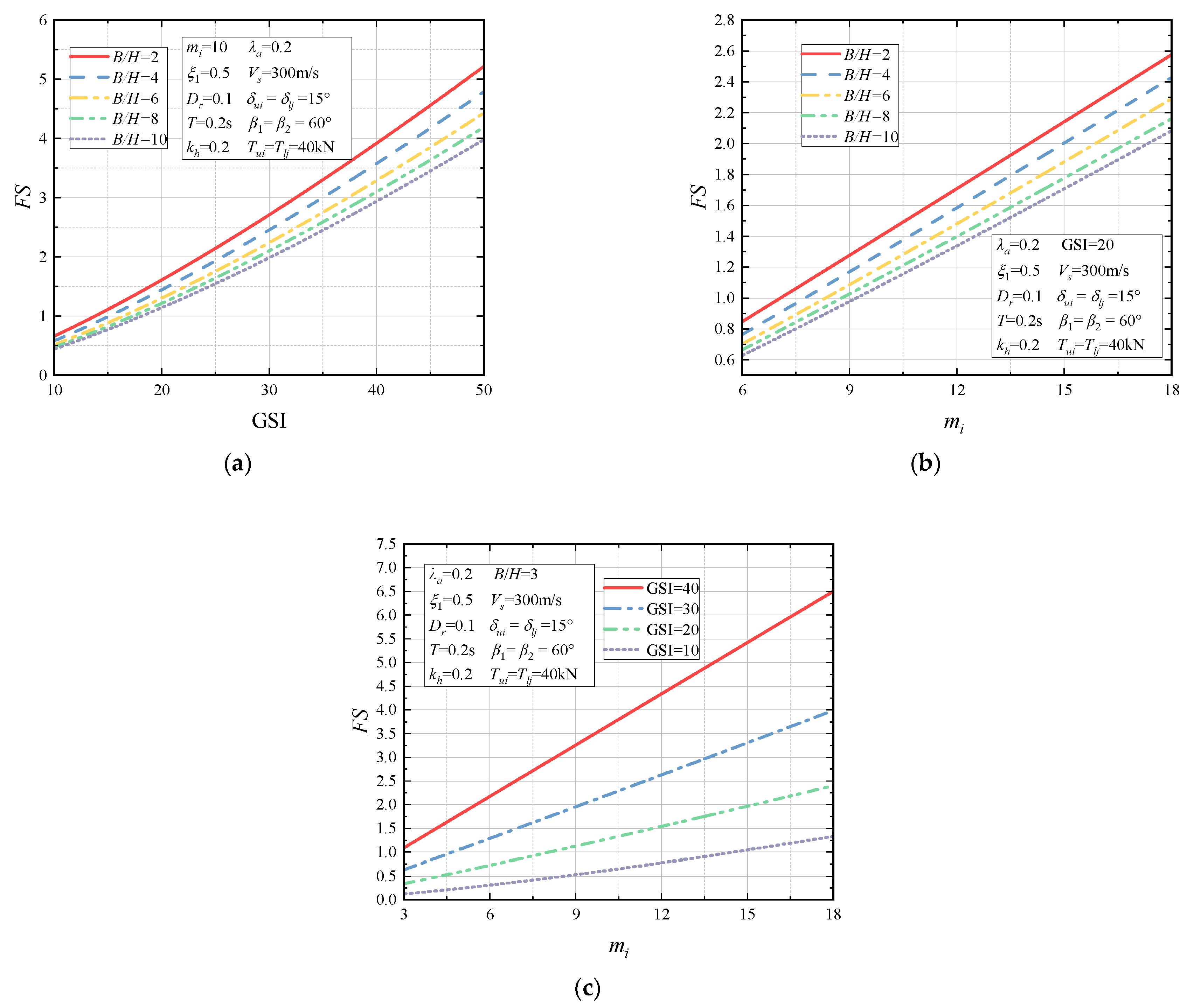
As shown in Figure 7, the Geological Strength Index $GSI$ and the parameter for the class of rock substance $m_i$ are proportional to FS, i.e., the larger that $GSI$ and $m_i$ are, the higher the stability of the slope, where the FS rise is more noticeable in Figure 7a. In the $GSI$ rating system, the value of $GSI$ is determined by the structure of the rock mass and the quality condition of the structural surface,

Under the rating system, the quality conditions of the structural surface influence the value of $GSI$, from which it can be observed that the overall quality of the rock mass has more of an impact on the stability of rock slopes than the quality characteristics of the rock in the stability analysis of the rock slopes. Thus, special attention should be paid to both the structure of the rock mass and the quality condition of the structural face in the engineering design.

Furthermore, the fall in FS with an increase in B/H occurs when nonlinear H-B criteria factors are maintained. This indicates that, given the same other factors, 3D slopes are more stable than 2D slopes. This shows that it is overly cautious to simply handle the 3D slope in actual engineering as if it were just a 2D case. Additionally, Figure 7c shows the trend of FS with $m_i$ for different values of $GSI$. And it can be noticed that the FS growth amplitude is also small when the $GSI$ is small, implying that the rock type and quality do not significantly enhance the stability of the rock slopes when the joint fractures in the rock mass are excessively developed.

Figure 7. Impacts of nonlinear H-B criterion parameters on the safety of 3D two-stage rock slopes: (a) the Geological Strength Index $GSI$; (b) the parameter for the class of rock substance $m_i$; (c) the interactions between $GSI$ and $m_i$.

Figure 7. Impacts of nonlinear H-B criterion parameters on the safety of 3D two-stage rock slopes: (a) the Geological Strength Index $GSI$; (b) the parameter for the class of rock substance $m_i$; (c) the interactions between $GSI$ and $m_i$.

4.2.2. Improved Pseudo-Dynamic Parametric Analysis

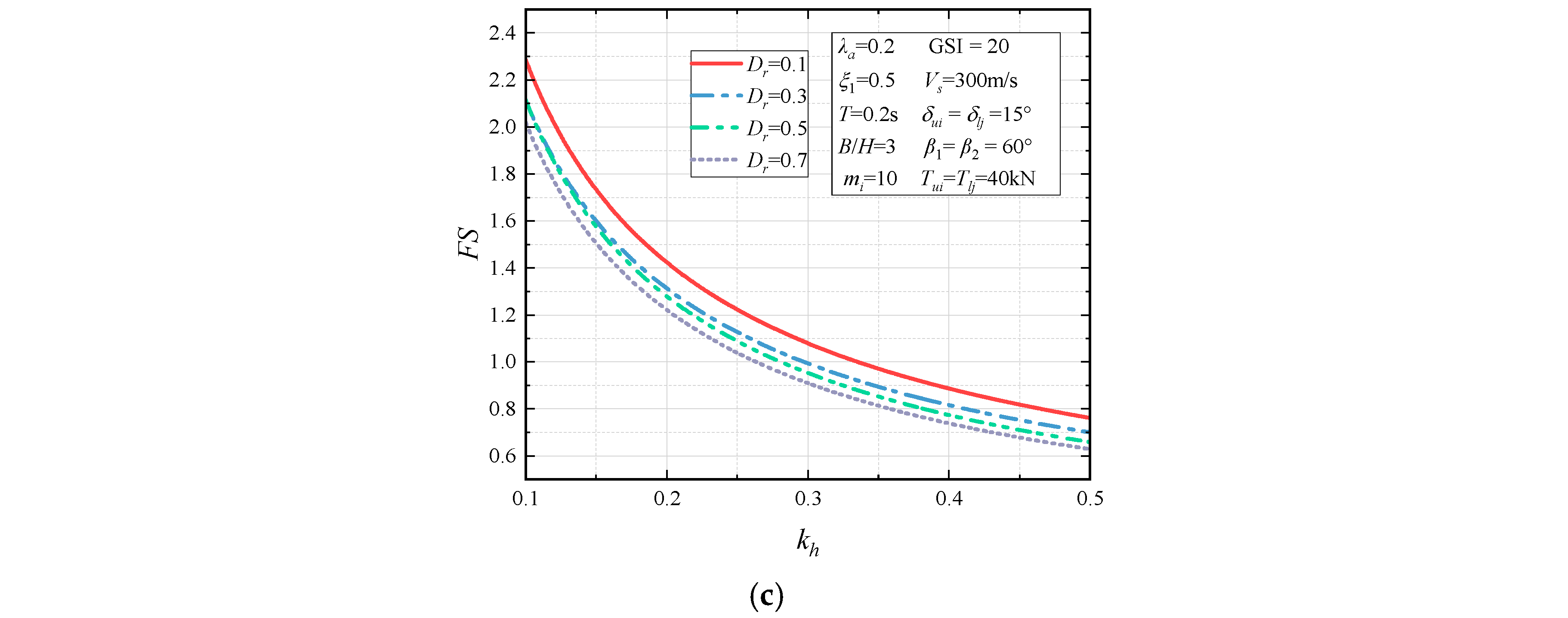
In Figure 8, the effects of several typically improved pseudo-dynamic factors on the safety for two-stage rock slopes as B/H varies are depicted. It can be seen that FS gradually decreases as the horizontal seismicity factor $k_h$, velocity of transverse wave propagating $V_s$, seismic period $T$, and damping ratio $D_r$ increase, respectively. But their reductions are not linear, i.e., it is as the value of the seismic pseudo-dynamic parameters change at smaller values that FS decreases more. For example, fixing B/H = 3, FS reduces by 35% as $k_h$ increases from 0.1 to 0.2, while FS decreases by less than 10% as $k_h$ increases from 0.4 to 0.5, as shown in Figure 8a. The findings demonstrate that the smaller magnitude of aftershocks is additionally significant for the slope reinforcement engineering. Then, Figure 9 exhibits the interactions of the horizontal seismicity coefficient $k_h$ with the rest of the modified pseudo-dynamic parameters. At arbitrary $k_h$ ($0.1\le k_h\le 0.5$), the variations of FS with the unit change for $V_s$, $T$, and $D_r$ are all minor and do not exceed 10%.

Figure 8. Effects of pseudo-dynamic parameters: (a) the horizontal seismicity factor $k_h$; (b) velocity of transverse wave propagating $V_s$; (c) seismic period $T$; (d) damping ratio $D_r$.

Figure 8. Effects of pseudo-dynamic parameters: (a) the horizontal seismicity factor $k_h$; (b) velocity of transverse wave propagating $V_s$; (c) seismic period $T$; (d) damping ratio $D_r$.

Figure 9. The interactions between the seismic pseudo-dynamic parameters of the safety of 3D two-stage rock slopes: (a) the reciprocal actions between $V_s$ and $k_h$; (b) the reciprocal actions between $T$ and $k_h$; (c) the reciprocal actions between $D_r$ and $k_h$.

Figure 9. The interactions between the seismic pseudo-dynamic parameters of the safety of 3D two-stage rock slopes: (a) the reciprocal actions between $V_s$ and $k_h$; (b) the reciprocal actions between $T$ and $k_h$; (c) the reciprocal actions between $D_r$ and $k_h$.

4.2.3. Slope Geometry Parametric Analysis

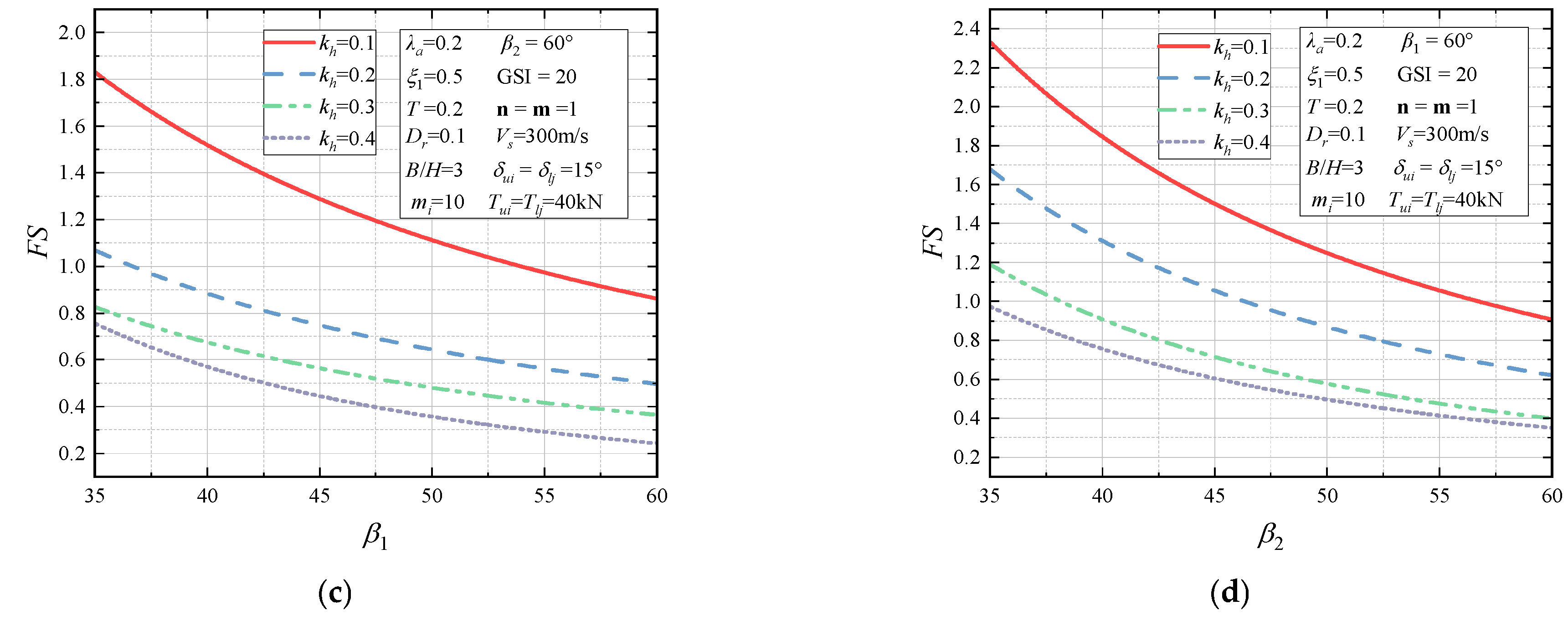
The influence of the slope geometry parameters on slope safety at different seismic classes is illustrated in Figure 10. It can be observed that the height coefficient ${\xi }_1$ and the factor of stage width ${\lambda }_a$ are favorably proportional to FS, while ${\beta }_1$ and ${\beta }_2$ are inversely proportional to FS. And it is noteworthy that the design pattern for the two-stage slope could significantly withstand the adverse effects of seismicity on slope safety, as shown in Figure 10a, and its enhancement on FS is more obvious when the seismicity is at a smaller level. Moreover, the location of the additional step on the middle and lower portions of the slope can better improve the stability of the slope, as demonstrated in Figure 10b. It is important to note that, at the same range of 35°–60°, the FS fluctuation magnitude relating to ${\beta }_2$ is greater than that of ${\beta }_1$, which implies that ${\beta }_2$ has a stronger impact on slope safety. And the above findings have some reference to the design for the two-stage rock slope.

Figure 10. Effects of slope geometry parameters: (a) the factor of stage width ${\lambda }_a$; (b) the height factor ${\xi }_1$; (c) inclined angle of upper stage ${\beta }_1$; (d) inclined angle of lower step ${\beta }_2$.

Figure 10. Effects of slope geometry parameters: (a) the factor of stage width ${\lambda }_a$; (b) the height factor ${\xi }_1$; (c) inclined angle of upper stage ${\beta }_1$; (d) inclined angle of lower step ${\beta }_2$.

4.2.4. Anchorage Parametric Analysis

When the anchorage force for each row of anchor cables is consistent, the critical anchorage force of the prestressed anchor cable can be derived by the variation of Equation (86):

$$T_{cr}=\frac{\gamma \cdot \left[g_3+g_4+k_h(g_5+g_6)-{\eta }_1{\lambda }_c\cos {\phi }_t(g_1+g_2)\right]}{{\displaystyle \sum _{i=1}^n{g}_{7i}+}{\displaystyle \sum _{j=1}^m{g}_{8j}}}$$

(88)

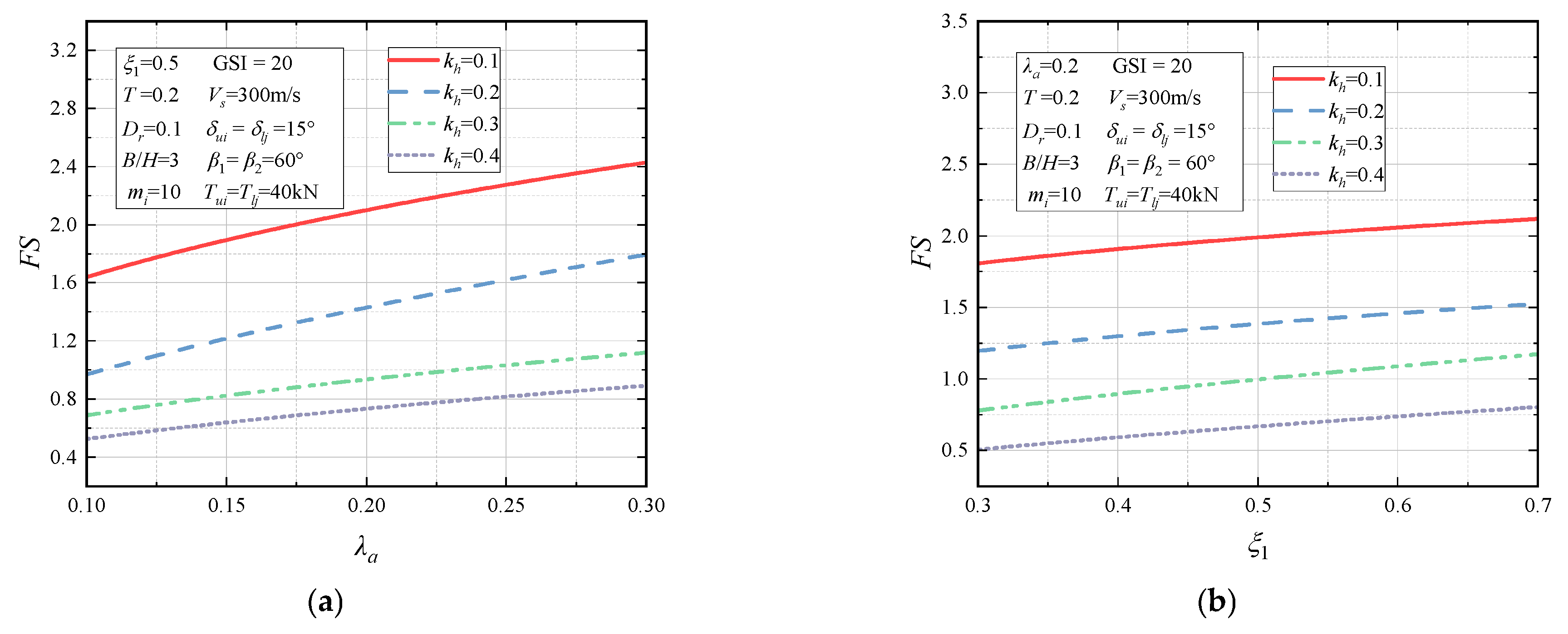
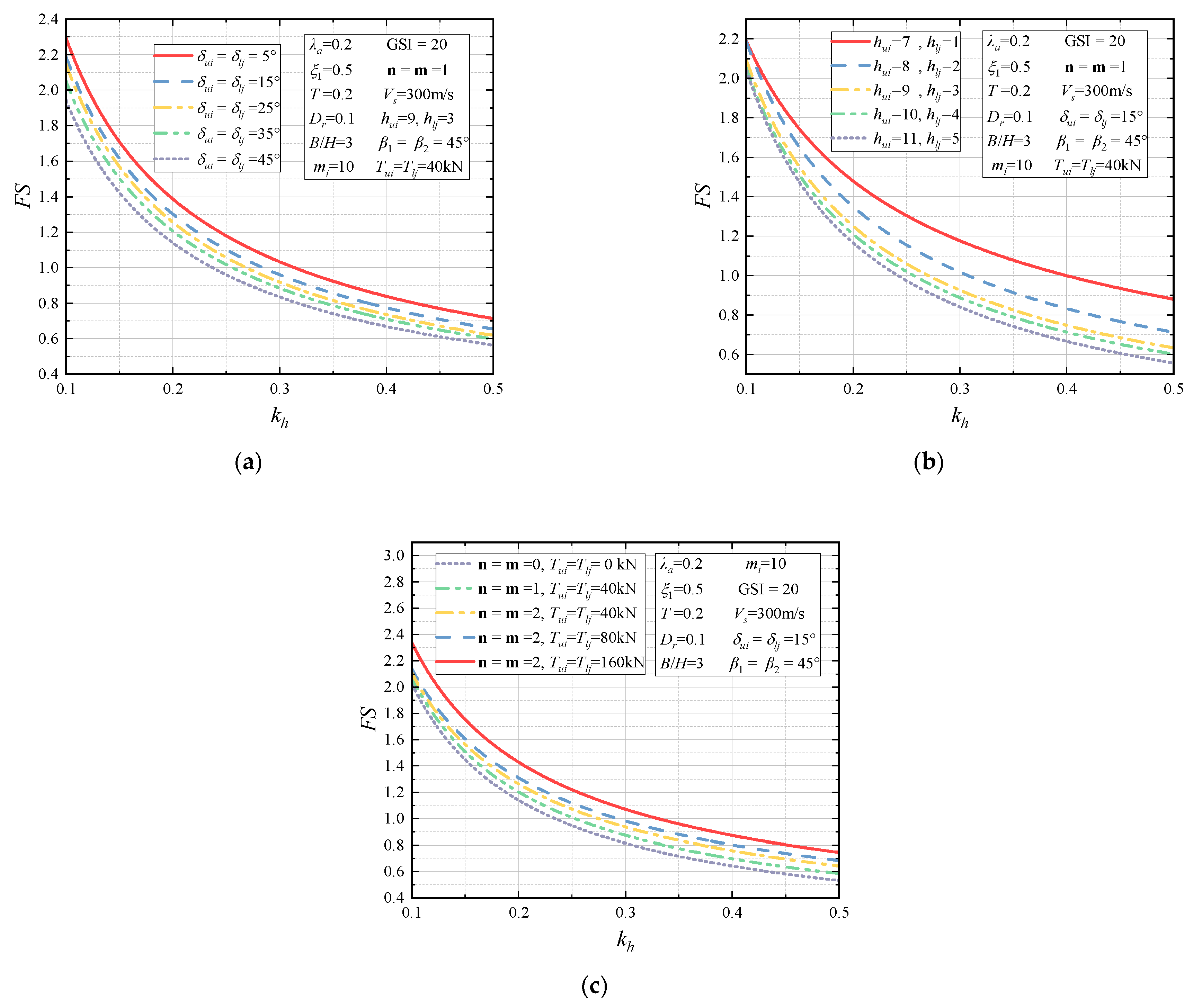
The above equation can provide the reference or verification basis for the anchorage design of rock slopes. Moreover, Figure 11 depicts the effects of prestressing anchorage parameters on the reinforcement of two-stage rock slopes with the variation in seismicity classes. It can be found that FS gradually reduces with the increase in the anchorage angles ${\delta }_{ui}$ and ${\delta }_{lj}$ and the anchor head heights $h_{ui}$ and $h_{lj}$, while the slope stability is progressively enhanced with the growth in the anchoring forces $T_{ui}$ and $T_{lj}$ and the number of anchor rows n and m. It is worth noting that the anchor head heights have little effect on the stability of the slope at small seismicity magnitudes, whereas the effect of the anchor cable arrangement at different heights on FS varies greatly at larger seismicity magnitudes, as illustrated in Figure 11b. In addition, Figure 11a shows that the slippage of the sliding body for the slope can be more effectively controlled with the anchorage angles close to horizontal. These indicate that the anchorage design is essential for the seismic stability of slopes.

Figure 11. Impacts of anchorage parameters on the safety of 3D two-stage rock slopes: (a) the anchorage angles ${\delta }_{ui}$ and ${\delta }_{lj}$; (b) the anchor head heights $h_{ui}$ and $h_{lj}$; (c) the number of anchor rows n and m, the anchoring forces $T_{ui}$ and $T_{lj}$.

Figure 11. Impacts of anchorage parameters on the safety of 3D two-stage rock slopes: (a) the anchorage angles ${\delta }_{ui}$ and ${\delta }_{lj}$; (b) the anchor head heights $h_{ui}$ and $h_{lj}$; (c) the number of anchor rows n and m, the anchoring forces $T_{ui}$ and $T_{lj}$.

5. Conclusions

According to the upper bound theorem of LA, this paper presents the new mathematical formula for the analytical solution of the seismic safety of the 3D two-stage rock slope reinforced with prestressed anchor cables governed by the nonlinear Hoek–Brown criterion, in which the analyses of seismicity are performed by the latest modified pseudo-dynamic method. And the 3D failure mechanism is employed to analyze and derive internal energy dissipation and external forces work within the failure model of two-stage rock slopes, where the power of the seismic force is calculated by the horizontal stratification method, and the work exerted by the anchor groups on the upper and lower stage surface is derived and calculated, separately. With these prerequisites, the factor of safety (FS) defined by the rate for internal energy dissipation and external force work can be collated as an explicit function of the five variables. And the precise analytical solution of FS can be found by combining it with the PSO algorithm.

To verify the correctness of the assessment model for the seismic safety for the 3D two-stage rock slope reinforced with prestressing anchor cables and the accuracy of the corresponding analytical solutions presented in this paper, the results were compared with those of the pertinent literature and other approaches, and the errors were all within the acceptable range. Subsequently, the sensitivity analyses and the coupling effects of the seismic pseudo-dynamic parameters and prestressing anchorage parameters within the kinematic model of the 3D two-stage rock slopes governed by the Hoek–Brown criterion were carried out. And the key findings are shown below.

(1)

For the rock mass characteristics, the analyses indicate that the overall quality of the rock mass has more of an impact on the stability of rock slopes than the quality characteristics of the rock in the stability analysis of the rock slopes. And the rock type and quality do not significantly enhance the stability of the rock slopes when the joint fractures in the rock mass are excessively developed.

(2)

For the seismicity factors, their variations with FS are not linear. And it is as the value of the seismic pseudo-dynamic parameters change at smaller values that FS decreases more, which demonstrates that the smaller magnitude of seismicity is also additionally significant for the slope reinforcement engineering.

(3)

For the slope geometry features, the design pattern for the two-stage slope could significantly withstand the adverse effects of seismicity on slope safety, and its enhancement on FS is more obvious when the seismicity is at a smaller level. Moreover, the location of the additional step on the middle and lower portions of the slope can better improve the stability of the slope.

(4)

Equation (87) can provide the reference or verification basis for the anchorage design of rock slopes. For the prestressing anchorage parameters, the slope stability is progressively enhanced with the growth of the anchoring forces $T_{ui}$ and $T_{lj}$ and the number of anchor rows n and m. Additionally, the slippage of the sliding body for the slope can be more effectively controlled with the anchorage angles close to horizontal. These indicate that the anchorage design is essential for the seismic stability of slopes.

References

- Jiang, S.H.; Li, D.Q.; Zhang, L.M.; Zhou, C.B. Time-dependent system reliability of anchored rock slopes considering rock bolt corrosion effect. Eng. Geol. 2004, 175, 1–8. [Google Scholar] [CrossRef]
- Blanco-Fernandez, E.; Castro-Fresno, D.; Díaz, J.D.C.; Lopez-Quijada, L. Flexible systems anchored to the ground for slope stabilisation: Critical review of existing design methods. Eng. Geol. 2011, 122, 129–145. [Google Scholar] [CrossRef]
- Eskandarinejad, A. Seismic vertical uplift capacity of horizontal strip anchors embedded in sand adjacent to slopes using finite element limit analysis. Arab. J. Geosci. 2022, 15, 16. [Google Scholar] [CrossRef]
- Sun, J.; Yu, T.; Dong, P. Pseudo-dynamic analysis of reinforced slope with anchor cables. Soil Dyn. Earthq. Eng. 2022, 162, 107514. [Google Scholar] [CrossRef]
- Tao, Z.; Zhu, C.; He, M.; Karakus, M. A physical modeling-based study on the control mechanisms of Negative Poisson’s ratio anchor cable on the stratified toppling deformation of anti-inclined slopes. Int. J. Rock Mech. Min. Sci. 2021, 138, 104632. [Google Scholar] [CrossRef]
- Chen, J.F.; Du, C.C.; Peng, M.; Sun, R.; Zhao, F.; Shi, Z.M. System reliability analysis of a slope stabilized with anchor cables and piles under seismic loading. Acta Geotech. 2023, 18, 4493–4514. [Google Scholar] [CrossRef]
- Zhang, Z.L.; Yang, X.L. Unified solution of safety factors for three-dimensional compound slopes considering local and global instability. Comput. Geotech. 2023, 155, 105227. [Google Scholar] [CrossRef]
- Zhong, J.H.; Yang, X.L. Seismic stability of three-dimensional slopes considering the nonlinearity of soils. Soil Dyn. Earthq. Eng. 2021, 140, 106334. [Google Scholar] [CrossRef]
- Zhang, S.; Xu, Q.; Peng, D.; Zhu, Z.; Li, W.; Wong, H.; Shen, P. Stability analysis of rock wedge slide subjected to ground water dynamic evolution. Eng. Geol. 2020, 270, 105528. [Google Scholar] [CrossRef]
- Xu, S.; Zhou, D. An Analytical Framework for Assessing the Unsaturated Bearing Capacity of Strip Footings under Transient Infiltration. Mathematics 2023, 11, 3480. [Google Scholar] [CrossRef]
- Kang, X.D.; Zhou, D. Analytical Solution for Bearing Capacity of Reinforced Strip Footings on Unsaturated Soils under Steady Flow. Mathematics 2023, 11, 3746. [Google Scholar] [CrossRef]
- Griffiths, D.V.; Marquez, R.M. Three-dimensional slope stability analysis by elasto-plastic finite elements. Géotechnique 2007, 57, 537–546. [Google Scholar] [CrossRef]
- Yang, X.L.; Yin, J.H. Slope stability analysis with nonlinear failure criterion. J. Eng. Mech. 2004, 130, 267–273. [Google Scholar] [CrossRef]
- Yang, X.L.; Wang, J.M. Ground movement prediction for tunnels using simplified procedure. Tunn. Undergr. Space Technol. 2011, 26, 462–471. [Google Scholar] [CrossRef]
- Yang, X.L.; Huang, F. Collapse mechanism of shallow tunnel based on nonlinear Hoek-Brown failure criterion. Tunn. Undergr. Space Technol. 2011, 26, 686–691. [Google Scholar] [CrossRef]
- Giger, M.W.; Krizek, R.J. Stability analysis of vertical cut with variable corner angle. Soils Found. 1975, 15, 63–71. [Google Scholar] [CrossRef]
- De Buhan, P.; Garnier, D. Three dimensional bearing capacity analysis of a foundation near a slope. Soils Found. 1998, 38, 153–163. [Google Scholar] [CrossRef] [PubMed]
- Michalowski, R.L.; Drescher, A. Three-dimensional stability of slopes and excavations. Géotechnique 2009, 59, 839–850. [Google Scholar] [CrossRef]
- Zhong, J.H.; Yang, X.L. Pseudo-dynamic stability of rock slope considering Hoek-Brown strength criterion. Acta Geotech. 2021, 17, 2481–2494. [Google Scholar] [CrossRef]
- Hoek, E.; Brown, E.T. Empirical strength criterion for rock masses. J. Geotech. Eng. Div. 1980, 106, 1013–1035. [Google Scholar] [CrossRef]
- Hoek, E.; Wood, D.; Shah, S. A modified Hoek–Brown failure criterion for jointed rock masses. In Rock Characterization: ISRM Symposium, Eurock’92, Chester, UK, 14–17 September 1992; Thomas Telford Publishing: London, UK, 1992; pp. 209–214. [Google Scholar]
- Hoek, E.; Carranza-Torres, C.; Corkum, B. Hoek-Brown failure criterion-2002 edition. Proc. NARMS-Tac 2002, 1, 267–273. [Google Scholar]
- Yang, X.L.; Yin, J.H. Upper bound solution for ultimate bearing capacity with a modified Hoek-Brown failure criterion. Int. J. Rock Mech. Min. Sci. 2005, 42, 550–560. [Google Scholar] [CrossRef]
- Yang, X.L.; Li, L.; Yin, J.H. Seismic and static stability analysis for rock slopes by a kinematical approach. Géotechnique 2004, 54, 543–549. [Google Scholar] [CrossRef]
- Loukidis, D.; Bandini, P.; Salgado, R. Stability of seismically loaded slopes using limit analysis. Géotechnique 2003, 53, 463–479. [Google Scholar] [CrossRef]
- Brink, U.T.; Andrews, B.; Miller, N. Seismicity and sedimentation rate effects on submarine slope stability. Geology 2016, 44, 563–566. [Google Scholar] [CrossRef]
- Macedo, J.; Candia, G.; Lacour, M.; Liu, C. New developments for the performance-based assessment of seismically-induced slope displacements. Eng. Geol. 2020, 277, 105786. [Google Scholar] [CrossRef]
- Michalowski, R.L.; Martel, T. Stability charts for 3D failures of steep slopes subjected to seismic excitation. J. Geotech. Geoenviron. Eng. 2011, 137, 183–189. [Google Scholar] [CrossRef]
- Li, Z.W.; Yang, X.L.; Li, T.Z. Static and seismic stability assessment of 3D slopes with cracks. Eng. Geol. 2020, 265, 105450. [Google Scholar] [CrossRef]
- Steedman, R.S.; Zeng, X. The influence of phase on the calculation of pseudo-static earth pressure on a retaining wall. Géotechnique 1990, 40, 103–112. [Google Scholar] [CrossRef]
- Zeng, X.; Steedman, R.S. On the behaviour of quay walls in earthquakes. Géotechnique 1993, 43, 417–431. [Google Scholar] [CrossRef]
- Bellezza, I. A new pseudo-dynamic approach for seismic active soil thrust. Geotech. Geol. Eng. 2014, 32, 561–576. [Google Scholar] [CrossRef]
- Bellezza, I. Seismic active earth pressure on walls using a new pseudo-dynamic approach. Geotech. Geol. Eng. 2015, 33, 795–812. [Google Scholar] [CrossRef]
- Chanda, N.; Ghosh, S.; Pal, M. Analysis of slope using modified pseudo-dynamic method. Int. J. Geotech. Eng. 2018, 12, 337–346. [Google Scholar] [CrossRef]
- Shi, K.; Wu, X.; Liu, Z.; Dai, S. Coupled calculation model for anchoring force loss in a slope reinforced by a frame beam and anchor cables. Eng. Geol. 2019, 260, 105245. [Google Scholar] [CrossRef]
- Li, X.; He, S.; Wu, Y. Limit analysis of the stability of slopes reinforced with anchors. Int. J. Numer. Anal. Methods Geomech. 2012, 36, 1898–1908. [Google Scholar] [CrossRef]
- Yan, M.; Xia, Y.; Liu, T.; Bowa, V.M. Limit analysis under seismic conditions of a slope reinforced with prestressed anchor cables. Comput. Geotech. 2019, 108, 226–233. [Google Scholar] [CrossRef]
- Li, A.J.; Lyamin, A.V.; Merifield, R.S. Seismic rock slope stability charts based on limit analysis methods. Comput. Geotech. 2009, 36, 135–148. [Google Scholar] [CrossRef]
- Kokane, A.K.; Sawant, V.A.; Sahoo, J.P. Seismic stability analysis of nailed vertical cut using modified pseudo-dynamic method. Soil Dyn. Earthq. Eng. 2020, 137, 106294. [Google Scholar] [CrossRef]
- Agarwal, E.; Pain, A. Probabilistic stability analysis of geosynthetic-reinforced slopes under pseudo-static and modified pseudo-dynamic conditions. Geotext. Geomembr. 2021, 49, 1565–1584. [Google Scholar] [CrossRef]
- Xu, S.; Zhou, D. Seismic Bearing Capacity Solution for Strip Footings in Unsaturated Soils with Modified Pseudo-Dynamic Approach. Mathematics 2023, 11, 2692. [Google Scholar] [CrossRef]
- Zhang, Z.L.; Yang, X.L. Seismic stability analysis of slopes with cracks in unsaturated soils using pseudo-dynamic approach. Transp. Geotech. 2021, 19, 100583. [Google Scholar] [CrossRef]
- Qin, C.B.; Chian, S.C. Kinematic analysis of seismic slope stability with a discretisation technique and pseudo-dynamic approach: A new perspective. Géotechnique 2018, 68, 492–503. [Google Scholar] [CrossRef]
- Gazetas, G.; Garini, E.; Anastasopoulos, I.; Georgarakos, T. Effects of near-fault ground shaking on sliding systems. J. Geotech. Geoenviron. Eng. 2009, 135, 1906–1921. [Google Scholar] [CrossRef]
- Yang, Y.; Zhou, D. Seismic Stability for 3D Two-Step Slope Governed by Non-Linearity in Soils Using Modified Pseudo-Dynamic Approach. Appl. Sci. 2022, 12, 6482. [Google Scholar] [CrossRef]
- Yang, Y.; Liao, H.; Zhu, J. Stability Analysis of Three-Dimensional Tunnel Face Considering Linear and Nonlinear Strength in Unsaturated Soil. Appl. Sci. 2024, 14, 2080. [Google Scholar] [CrossRef]
- Chen, G.; Chen, T.; Chen, Y.; Huang, R.; Liu, M. A new method of predicting the prestress variations in anchored cables with excavation unloading destruction. Eng. Geol. 2018, 241, 109–120. [Google Scholar] [CrossRef]
- Cheng, Y.; Xu, Y.; Wang, L.; Wang, L. Stability of expansive soil slopes reinforced with anchor cables based on rotational-translational mechanisms. Comput. Geotech. 2022, 146, 104747. [Google Scholar] [CrossRef]
- Qiang, L. Stability Study for Rock Slope and Anchoring Parametric Analysis. Ph.D. Thesis, Central South University, Changsha, China, 2010. [Google Scholar]
Figure 1.
The envelope curve of the nonlinear H-B yield criterion and its outer tangent.
Figure 2.
Three-dimensional horn-shaped rotating model for stepped rock slope reinforced with anchor groups.
Figure 3.
Stereoscopic diagram for 3D failure mechanism with the plane strain block and anchor group reinforcement.
Figure 4.
Schematic of the derivation of internal energy dissipation with local coordinate systems.
Figure 5.
Diagram of the horizontal stratification method: (a) full graph; (b) detail zoom.
Figure 6.
Schematic layout of anchor groups on the upper step slope and lower step slope.