Abstract
An essential component of autonomous transportation system management and decision-making is precise and real-time traffic flow forecast. Predicting future traffic conditionsis a difficult undertaking because of the intricate spatio-temporal relationships involved. Existing techniques often employ separate modules to model spatio-temporal features independently, thereby neglecting the temporally and spatially heterogeneous features among nodes. Simultaneously, many existing methods overlook the long-term relationships included in traffic data, subsequently impacting prediction accuracy. We introduce a novel method to traffic flow forecasting based on the combination of the feature-augmented down-sampling dynamic graph convolutional network and multi-head attention mechanism. Our method presents a feature augmentation mechanism to integrate traffic data features at different scales. The subsampled convolutional network enhances information interaction in spatio-temporal data, and the dynamic graph convolutional network utilizes the generated graph structure to better simulate the dynamic relationships between nodes, enhancing the model’s capacity for capturing spatial heterogeneity. Through the feature-enhanced subsampled dynamic graph convolutional network, the model can simultaneously capture spatio-temporal dependencies, and coupled with the process of multi-head temporal attention, it achieves long-term traffic flow forecasting. The findings demonstrate that the ADDGCN model demonstrates superior prediction capabilities on two real datasets (PEMS04 and PEMS08). Notably, for the PEMS04 dataset, compared to the best baseline, the performance of ADDGCN is improved by 2.46% in MAE and 2.90% in RMSE; for the PEMS08 dataset, compared to the best baseline, the ADDGCN performance is improved by 1.50% in RMSE, 3.46% in MAE, and 0.21% in MAPE, indicating our method’s superior performance.
1. Introduction
Traffic congestion has worsened due to rapid urbanization and an increase in private automobile ownership. Alleviating traffic congestion has emerged as a pressing concern in many countries. Moreover, frequent traffic jams and unplanned disruptions caused by accidents and emergencies significantly impede the smooth operation of road networks [1]. Consequently, the implementation of accurate and reliable traffic prediction models has become essential in enhancing the precision and effectiveness of traffic flow forecasting.
Intelligent transportation systems, as effective solutions to address traffic challenges, have garnered significant research attention in the transportation field. Among them, traffic flow forecasting has received considerable focus. Traffic forecasting represents a specific case of spatio-temporal data prediction, aiming to forecast future traffic characteristics like flow rate and speed by using past traffic records [2]. However, traffic flow predicting is complex because of intricate spatio-temporal dependencies, presenting significant challenges for accurate and real-time predictions.
Unlike traditional time series analysis, traffic forecasting is influenced by various external factors, including spatial factors [3]. As shown in Figure 1, in the temporal dimension, the mobility behaviors of urban residents result in clear cyclical patterns in overall traffic flow [4]. Moreover, traffic flows are susceptible to volatility caused by external variables such as events or traffic accidents, which cannot be avoided. In the spatial dimension, traffic information propagates through the structure of the road system. For instance, the flow of traffic on particular roads directly affects the movement of vehicles on adjacent roads, highlighting the transient and dynamic nature of traffic [5]. Spatio-temporal correlation also exhibits multi-scale characteristics, encompassing global and local features in spatial dimensions and long-term and short-term dynamics in temporal dimensions [6]. These characteristics have significant implications for understanding and predicting traffic flow changes.
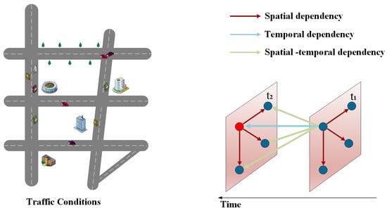
Figure 1.
The intricate spatio-temporal relationship of the traffic road network.
Deep learning techniques have been extensively employed in recent years to investigate the spatio-temporal relationships of traffic data. Graph neural networks (GNNs) [7] have provided a viable approach for modeling non-Euclidean spatio-temporal networks. Models like STGCN [8], T-GCN [9] and DCRNN [10] combine recurrent neural networks with graph convolutional networks to model spatio-temporal relationships. STGNN [11] introduces GRU and Transformer architectures to handle local and global temporal correlations. However, these approaches rely on prior knowledge of the graph structure [12] and fail to fully account for dynamic changes and heterogeneity in spatio-temporal data. STSGCN [13] proposes the dynamic learning of spatial information over time by constructing local spatio-temporal graphs but overlooks the capture of temporal information. AGCRN [14] and DGCRN [15] use adaptive graph generation with gated cyclic units to capture spatio-temporal heterogeneity but lack attention to global information. Although these methods improve traffic prediction performance from various perspectives, they often capture temporal and spatial correlations independently, which may weaken the captured spatio-temporal correlations or even amplify irrelevant features. Recent studies such as AFDGCN [16] aim to model temporal and spatial relationships synchronously via spatial module embeddings, making a positive contribution to the model. Nevertheless, these approaches are constrained in effectively capturing the interactive learning of spatial–temporal information, which affects the models’ ability to make predictions.
In order to overcome the shortcomings of the current approaches, we provide an approach based on the combination of a feature-augmented down-sampling dynamic graph convolutional network and multi-head attention mechanism for predicting traffic flow. The down-sampling dynamic graph convolution network and multi-head attention mechanism based on feature augmentation are used to learn complex traffic change relationships at a multi-scale spatio-temporal level. The following are the principal contributions of this study:
- A new spatio-temporal forecasting model ADDGCN is put forward. This model introduces a feature augmentation mechanism to fuse features of different scales, and embeds dynamic graph convolution into the down-sampling convolution network so that the model can simultaneously capture time and spatial correlation. Through the down-sampling dynamic graph convolution network based on feature augmentation, the spatio-temporal dependency is accurately captured by the model and, combined with the multi-head temporal attention mechanism, achieves long-term prediction of traffic flow.
- A down-sampling dynamic graph convolution module (DS-DGC) is designed. Among them, the down-sampling convolution network can enhance the information interaction of spatio-temporal data, and the dynamic graph convolution network can use the generated graph structure to better simulate the dynamic correlation among nodes, which is essential to improve the model’s ability to depict spatial heterogeneity.
- Extensive tests are conducted on two authentic traffic datasets and compared with 11 baseline models. The experimental findings demonstrate that our proposed approach surpasses these baseline techniques across three standard evaluation metrics.
This paper provides a summary of related work on traffic flow forecasting in Section 2, followed by the framework of the model and problem descriptions in Section 3. Section 4 provides a detailed explanation of our proposed model, ADDGCN. Section 5 showcases the analytical and experimental findings. Lastly, Section 6 offers conclusions and prospects for further research.
2. Related Works
To address the numerous difficulties and challenges in traffic forecasting, extensive research has been conducted by numerous scholars. Deep learning techniques and traditional methodologies make up the two main categories of current traffic forecast methods.
2.1. Traditional Method
Early time series tasks utilized statistical models such as HA [17], VAR [18], and ARIMA [19]. These methods required data to conform to specific stationarity assumptions, making them unsuitable for capturing non-linear variations in traffic data. In comparison to methods based on machine learning, these models exhibited subpar performance. Later, machine learning methods, including SVR [20], KNN [21] and XGBoost [22], were developed to study the non-linearity of traffic flow. However, they necessitated manual feature engineering and faced challenges in incorporating spatial information, thus limiting their feature-processing capabilities.
2.2. Deep Learning Method
As deep learning models are developing rapidly, RNN and its derivatives like LSTM and GRU have demonstrated excellent performance in time series tasks. Ma et al. [23] pioneered the application of LSTM in predicting traffic speed, enhancing the modeling capabilities for long-sequence correlations and effectively addressing the gradient issues of disappearing and exploding. Cui et al. [24] introduced a novel approach for forecasting traffic speed that utilizes stacked bidirectional and unidirectional LSTM to capture the correlations between preceding and subsequent time sequences. However, RNN models treat different road sequences as discrete data streams, focusing solely on the temporal relationships and neglecting the spatial relationships in traffic prediction. Additionally, RNN models suffer from slow convergence during training and struggle to effectively handle long time series data.
To overcome these limitations, CNNs have been widely applied as an alternative approach to time series processing as seen in models like WaveNet [25] and TCN [26]. Recently, Liu et al. introduced SCINet [27], which increased the receptive field of convolutional operations and utilized down-sampling interactive convolutions to enable multi-resolution analysis, achieving outstanding performance in traffic prediction. However, SCINet overlooks the spatial correlations present in traffic data. CNNs have been used in several research works to try to extract spatial correlations from traffic data. For instance, Zhai et al. [28] presented STResNet, which employs a CNN-based deep residual network for effective urban population flow forecasting. Narmadha et al. [29] introduced a spatio-temporal dynamic network that combined CNN and LSTM to handle spatio-temporal information for taxi and bike flow prediction in New York. Nevertheless, CNNs rasterize graph data and fail to consider the unique topological structure of transportation networks, making them unsuitable for non-Euclidean traffic data and less effective in learning complex spatial relationships for traffic prediction tasks.
Given the non-Euclidean characteristics of transportation networks, GCN has been extensively applied to traffic prediction tasks. GCN can be categorized into spectral-based GCN and frequency-based GCN. Bruna et al. [30] first introduced spectral-based generalized GCN, which utilized Fourier transformation to map the topological graph structure from spatial domain to spectral domain for convolutional operations and then reverse-transformed to finish the GCN process in the spatial domain. Defferrard et al. [31] enhanced classical GCN by proposing ChebNet to simplify Laplacian computation. Zhao et al. [9] proposed a model called T-GCN for spatio-temporal traffic forecasting, employing GCN and GRU to separately learn temporal and spatial dependencies. Yu et al. [8] presented STGCN, which utilized CNN to learn temporal relationships and GCN to model spatial relationships. Bai et al. [32] introduced STG2Seq, which incorporated two attention-based gated residual GCN modules to simulate spatio-temporal correlations. These methods, incorporating graph convolutional neural networks, directly perform convolutional operations on traffic data, leading to significant improvements in predictive performance.
3. System Model and Definitions
Traffic flow predicting utilizes historical traffic observation data to make predictions about how the traffic flow will vary in the future. Given a road system, it is characterized by , where is the collection of all observation points in the traffic road system, wherein v represents each observation point (i.e., sensor), E is the set of sides connecting two nodes in V, and the edges’ weights correspond to the actual distance of each node. The adjacency matrix symbolizes the connection relationships of each edge in graph G. Assuming the given historical traffic sequence is represented as , the predicted future traffic sequence can be represented as , where represents the characteristic attributes of all nodes in graph G at time step t, with T representing the length of the specified historical time sequence, and C representing the quantity of feature channels. symbolizes the length of the time sequence to be forecasted. The following is a definition of the traffic flow forecast problem:
where presents a learnable mapping function based on parameter matrix , which maps historical sequences to predicted sequences.
4. Our Proposed ADDGCN System
The ADDGCN model’s architecture as depicted in Figure 2 comprises three modules: a diffuse graph convolution module, a down-sampling dynamic graph convolution module based on feature augmentation, and a multi-head attention module. The core ideas can be summarized as (1) the fusion of adaptive adjacency matrix and learnable adjacency matrix to construct a dynamic graph structure; (2) using a down-sampling dynamic graph convolution module to simultaneously learn spatio-temporal relationships while modeling the spatial heterogeneity of spatio-temporal sequences; and (3) using a multi-head attention machine to record traffic data dependencies over lengthy periods of time.
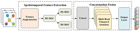
Figure 2.
ADDGCN overall structure diagram.
4.1. Down-Sampling Dynamic Graph Convolution Module Based on Feature Augmentation
4.1.1. Feature Augmentation
Due to the correlation among multiple features of traffic data, different features have varying effects on predicting traffic flow. In order to obtain a thorough comprehension of the inherent properties of time series data, this study introduces a feature augmentation layer utilizing a channel attention mechanism [33]. This layer consists of two submodules: temporal attention and channel attention. The channel attention submodule employs two multi-layer perceptrons to compress the input feature map, thereby rescaling features with a lower-dimensional distribution. Individual activation processes and self-threshold mechanisms are utilized to analyze the influence of each channel, determining the importance of each channel. Finally, the compressed feature maps are fused through an element-wise product and the ReLU activation function to obtain enhanced channel attention features. The temporal attention [34] submodule performs temporal feature fusion by using two 1D convolutional layers. Similar to the submodule for channel attention, this submodule determines the importance of each time point through the element product and sigmoid activation function, uses the convolution kernel to fuse the temporal features, and finally acquires the enhanced temporal attention features. The configuration of the feature enhancement module can be observed in Figure 3.
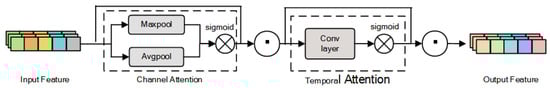
Figure 3.
Feature augmentation module structure diagram.
Assuming a given input feature map is , the channel attention submodule can be expressed as:
where ⊙ stands for the multiplication of elements, represents the sigmoid function, and and represent the fully linked layer’s weight parameters and biases. The input feature map is processed through the channel attention submodule. The temporal attention submodule can be expressed as:
where is the convolution kernel. After is preprocessed, the weighted feature graph is used as the feature enhancement module ’s result for subsequent model training.
The feature enhancement layer is based on the “squeeze excitation” structure [35]. It not only combines characteristics from varying scales but also automatically learns the importance of different features, enhancing the representation of feature maps.
4.1.2. Down-Sampling Dynamic Graph Convolution Network
Figure 4 presents the structure of the down-sampling dynamic graph convolution (DS-DGC) module [36], comprising a down-sampling convolution network and a dynamic graph convolution network (DGCN). The down-sampling convolutional network comprises fundamental down-sampling blocks arranged in a binary tree structure. If necessary, more down-sampling blocks can be stacked to increase the prediction accuracy. At the same time, to augment the model’s ability to simultaneously capture spatio-temporal correlation, the DGCN module is incorporated into the down-sampling convolution structure to use the captured spatial information to assist in the training process.
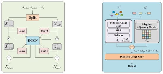
Figure 4.
Down-sampling convolution structure diagram and dynamic graph convolution structure diagram. Down-sampling dynamic graph convolutional network structure diagram on the left, and dynamic graph convolution structure graph on the right.
Let serve as the down-sampling convolution module’s input. The sequence data are decomposed into odd sequence and even sequence through the sequence decomposition operation, which not only reduces the number of data but also largely preserves the original sequence’s information. Next, four convolutional networks , , , and are used to interactively obtain the two subsequences’ respective feature information from the input sequence. Following the initial interactive learning, the output is and , the and continue to learn interactively, and the final output is and .
The operations in the down-sampling convolution module are characterized as:
where is the dynamic graph convolution, tanh is the stimulation function, and ⊙ represents the Hadamard product.
The dynamic graph convolution module’s design is depicted in Figure 4, where the central component is a graph generator and the diffusion graph convolution network. The initial adjacency matrix and the hidden feature are input into the graph generator. The subsequent steps include applying diffusion graph convolution [37] and passing the result through a multi-layer perceptron to generate an adjacency matrix that incorporates spatio-temporal characteristics. The overall procedure can be summarized as follows:
where represents a diffusion graph convolution operation, and represents a multi-layer perceptron.
Since the produced matrix is discontinuous, we must utilize the Gumbel function to reparameterize it in order to verify that the sampling procedure can be derived [38]:
where is the eigenvalue of the softmax function, which is set to 0.5 here, and is a random variable. Dynamic relationships between nodes may be modeled using .
Along with the adjacency matrix created by the graph generator, we also build an adaptive adjacency matrix [39] . It can be expressed as:
where and represent learnable parameters, and we use the predetermined adjacency matrix A as the initial value of .
Finally, the adjacency matrix , obtained by fusing and , is input into the diffusion graph convolution. It is used to simulate the dynamic correlation [40] between nodes and explore hidden node relationships in the road system. The fusion process can be expressed as:
where represents the fused dynamic adjacency matrix, while represents the learnable adaptive parameter factor.
In this module, the input is segmented into two subsequences, labeled as and . The temporal information in both subsequences is fused using different 1D convolutions, ensuring the preservation of temporal integrity. The interactive learning strategy in the down-sampling convolution module allows two subsequences to capture each other’s spatio-temporal features, enhancing the interaction of temporal and spatial information and avoiding the loss of important information with the down-sampling method. Additionally, the DGCN module uses the generated graph structure to simulate the dynamic correlations that occur between nodes over time, improving the capacity of the model to represent spatial heterogeneity [41]. Embedding DGCN into the down-sampling convolutional network enables the model to capture the spatio-temporal correlation simultaneously.
4.2. Multi-Head Attention Mechanism
To effectively describe the enduring interdependence of traffic data, we develop a multi-head temporal attention layer [42] to model the global contextual information of time series. This layer, as shown in Figure 5, comprises a position embedding layer, a multi-head attention mechanism and a feed-forward network layer. The specific structure is illustrated in the figure. By utilizing the temporal attention mechanism, our model is more capable of learning longer-term temporal trends and discovering the worldwide traffic data information in the temporal dimension.
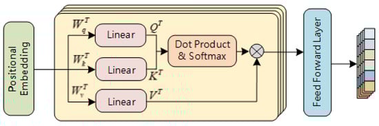
Figure 5.
Structural diagram of the multi-head temporal attention layer.
After undergoing processing by the DS-DGC module, two time subsequences and are obtained. Then, these subsequences are rearranged and combined in the order of their time indices to form a new time series, denoted as , which will be utilized as the multi-head temporal attention layer’s input. Considering the fact that the multi-head attention mechanism may not accurately account for the relative position in the sequence during the dot product operation, it is important to address this issue. At each time step, a position vector is added to the input data to overcome this issue:
where the of the position code is defined as:
First, the encoded input sequence is used to generate key matrix K, value matrix V, and the query matrix Q for the self-attention mechanism. The formulas are as follows:
where and are the learnable projection matrices. Next, the query matrix Q is multiplied by the transpose of the key matrix K, and the result is normalized to obtain the weight coefficient in the time dimension. Finally, the weight coefficient is applied to the value matrix V to obtain the weighted results of various time steps. This is the formula:
where denotes the weight scaling factor. To obtain the weighting of each variable, the attention scores are normalized using the softmax function.
The multi-head attention mechanism improves the model’s capacity to capture global temporal correlations [43], allowing it to focus on multiple subspace characteristics simultaneously. In the multi-head attention mechanism, multiple sets of self-attention operations are performed on the original input sequence, and their results are concatenated. Finally, the concatenated sequence is linearly transformed using the projection matrix to obtain the results of the multi-head attention mechanism. The equation is depicted as follows:
where is the linear transformation projection matrix. The feed-forward network layer receives the output of the multi-head attention layer and performs further processing on it. Residual links and layer normalization are used after each sublayer to optimize the model’s performance.
4.3. Diffusion Graph Convolutional Network
The diffusion graph convolution is employed twice in this model: once after the DS-DGC module and once in the dynamic graph convolution module. In DGCN, the diffusion graph convolution takes hidden features and a predefined initial adjacency matrix as input. Its definition is as follows:
where represents the parameter matrix. The diffusion map convolution used after the DS-DGC module aims to learn the spatio-temporal characteristics of the entire sequence data. Unlike the previous diffusion graph convolution, this module takes two matrices as input: the dynamic adjacency matrix and the predefined initial adjacency matrix . Furthermore, the multi-head attention layer’s input is also used as input for the diffusion graph convolution module. For directed graphs, the dissemination process entails bidirectional propagation, encompassing both forward and reverse. Therefore, for the initial adjacency matrix , its forward transition matrix and backward transition matrix can be represented as and correspondingly. Thus, the dissemination graph convolution module is as follows:
5. Performance Analysis
We conducted comprehensive testing on two actual datasets of highway traffic flow to assess the model’s performance.
5.1. Dataset
In this study, we utilized PEMS04 and PEMS08 [44], which are publicly accessible real-world traffic flow datasets. The California Department of Transportation deployed sensors to capture these statistics in real-time at a frequency of 30 s [45]. The collected data were then aggregated into 5 min time windows, producing 12 observations each hour. Table 1 contains comprehensive details about the datasets [46]. The distances between the sensors in these real traffic road networks were used to construct the adjacency matrices utilized in the experiments conducted in this study.

Table 1.
Detailed description of the dataset.
5.2. Experiment Settings
Prior to feeding the dataset into the model for training, the original data are uniformly standardized using the Z-Score normalization method [13]. Subsequently, the standardized data are split into three sets—a set for training, a set for validation, and a set for testing—following a 6:2:2 ratio. This study seeks to forecast 12 consecutive future time steps for the next hour by using data from 12 consecutive time steps in the preceding hour. During the experiments, the Ranger optimizer [47] is utilized. The batch size is configured as 64, with hidden dimensions set to 32. The model employs 4 attention heads during training, and the training process is conducted over 500 epochs. To prevent overfitting, an early stopping mechanism is used. The starting learning rate is set to 0.001.
We employ three standard metrics—Mean Absolute Error (MAE), Mean Absolute Percentage Error (MAPE), and Root Mean Square Error (RMSE)—to assess each approach’s efficacy [48], which are described as follows:
where N is the number of samples, indicates the predicted value, and indicates the true value.
5.3. Comparative Analysis of Results
Table 2 displays the comparative model and ADDGCN prediction results for two real traffic flow test datasets [16] for the next hour, consisting of 12 consecutive time steps. With the exception of the MAPE measure in PEMS04, which performs just slightly less well than SCINet, the proposed ADDGCN outperforms all baseline methods on both datasets. Specifically, on the PEMS04 dataset, ADDGCN demonstrates performance improvements of 2.46% and 2.90% in MAE and RMSE, in comparison to the best baseline model, accordingly. Similarly, for the PEMS08 dataset, ADDGCN achieves performance gains of 3.46%, 1.50%, and 0.21% in MAE, RMSE, and another metric, in comparison to the best baseline model, accordingly.
Table 2.
Comparing the performance of several models.
The results presented in Table 2 highlight the challenges faced by statistically based methods (HA, VAR) in handling non-linear and non-stationary time sequence data, leading to higher prediction errors. While deep learning methods, like TCN and LSTM, are superior to statistical models, they primarily concentrate on temporal correlations, ignoring the complex spatial relationships seen in traffic data. As a result, their modeling capabilities for spatio-temporal data are limited. On the other hand, models like STGCN and DCRNN incorporate GCN to extract spatial correlations, leading to better performance compared to time-based methods. By building adaptive or dynamic graph structures based on geographical correlations in historical data, AGCRN overcomes the drawbacks of fixed graph structures and achieves even higher prediction performance than earlier approaches. Graph WaveNet, which combines diffusion GCN with TCN, demonstrates exceptional ability in capturing temporal correlations, surpassing the performance of recently proposed models (SCINet, STG-NCDE). Notably, SCINet performs well even when spatial correlations are ignored, demonstrating the value of interactive learning. While STG-NCDE, a novel deep learning model, achieves promising results, it falls short compared to our proposed ADDGCN due to its sequential capture of spatio-temporal features. In contrast, our method employs a down-sampling interactive learning strategy to simultaneously capture spatio-temporal relationships. To imitate the dynamic links between nodes over time and study latent spatial relationships, the DGCN module looks into hidden node interactions in the road system. Moreover, our approach incorporates a feature enhancement module and attention mechanism to unveil multi-scale features and capture long-distance traffic fluctuation correlations.
To provide a clear visualization of the performance variances of the approach we propose and the baseline approaches, we depict the variations in MAPE, RMSE, and MAE for several methods on the two traffic datasets in Figure 6. Because MAPE, RMSE, and MAE are all indicators used to measure the size of prediction errors, the better our model performs in terms of predictions, the lower the values of these three indicators [49].
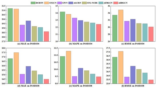
Figure 6.
Performance comparison of different models on the PEMS04 (above) and PEMS08 (below) datasets.
To better evaluate model performance, we selected two days with significant traffic fluctuations from the PEMS04 and PEMS08 datasets and conducted experiments using the traffic flow data. The comparison curves between the real traffic flow and the model-predicted flow for these two days are shown in Figure 7. The daypart is represented by the x-axis, while traffic flow numbers are represented by the y-axis. From Figure 7 [50], it is evident that our forecast model performs exceptionally well, correctly capturing the variations in traffic flow trends throughout the day. Furthermore, with the accurate understanding of traffic flow patterns, administrators can optimize the traffic management system, improve traffic efficiency, reduce congestion, and provide city residents with a more convenient commuting experience.
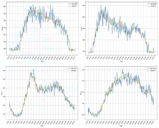
Figure 7.
Comparison of real value and predicted traffic flow in one day (traffic flow prediction of PEMS04 for 24 h (above). Traffic flow prediction of PEMS08 for 24 h (below)).
5.4. Ablation Study
We created five distinct versions of ADDGCN and ran ablation experiments on the PEMS04 and PEMS08 datasets, respectively, to learn more about how different components affect the ADDGCN prediction performance. The following are the variations:
(1) Without dynamic graph convolution network (DGCN): Based on ADDGCN, we replaced the DGCN module with an ordinary GCN module, and the input adjacency matrix of the GCN is the original matrix of adjacency.
(2) Without down-sampling convolution network: Based on ADDGCN, we removed the down-sampling convolution network.
(3) Without adapt adjacency (without ): Based on ADDGCN, we removed the adaptive adjacency matrix in the dynamic graph convolution network, leaving only as the adjacency matrix input to the diffusion graph convolution network.
(4) Without graph generator (without ): Based on ADDGCN, we removed the graph generator in the dynamic graph convolution network, leaving only as the adjacency matrix input to the diffusion graph convolution network.
(5) Without feature augmentation module: Based on ADDCN, we removed the feature augmentation module.
Table 3 displays the ablation experiment’s outcomes. The PEMS04 and PEMS08 datasets show essentially comparable distributions for the impacts of the above-discussed model components. Firstly, DGCN and down-sampling convolutional networks are very important to ADDGCN, which shows that our proposed DS-DGC module is crucial to improving the model prediction performance. Furthermore, ablation experiments were carried out on the two adjacency matrices that are described in the DGCN module. The experimental results demonstrate the critical roles played by the learnable adjacency matrix and the adaptive adjacency matrix in the model. The dynamic adjacency matrix is created by combining the adaptive adjacency matrix with the learnable adjacency matrix. This greatly enhances the prediction performance of ADDGCN. Finally, we experimented with the feature augmentation module using ablation. We can observe from the experimental data that after removing the feature augmentation module, the values of each indicator are also increased to varying degrees, and the prediction performance of ADDGCN is affected. It is evident that the feature augmentation module has a positive effect on our model. Therefore, our proposed DS-DGC module, combined with the feature augmentation module, is effective.
Table 3.
The impact of different components on ADDGCN prediction performance on the PEMS04 and PEMS08 datasets.
5.5. Impact of Different Hyperparameter Configurations
We carried out further studies on the PEMS04 and PEMS08 datasets to thoroughly assess the impact of hyperparameter settings. The ADDGCN model has only one hyperparameter related to its structure, which is the number of feature channels. This is because we did not use the strategy of stacking repeated modules to capture features. Results from experiments indicate that the effectiveness of the ADDGCN model is significantly affected by the number of feature channels as illustrated in Figure 8 [46]. However, adding more feature channels does not always result in an improvement in the performance of ADDGCN. Once the quantity of feature channels reaches a particular value, the performance of ADDGCN stabilizes. For the PEMS04 dataset, we found that the ADDGCN model performs best when the quantity of feature channels is approximately 64. On the other hand, for the PEMS08 dataset, the optimal number of feature channels is around 32. It is crucial to remember that the training time considerably rises along with the number of feature channels. As a result, we ultimately determined the number of feature channels in ADDGCN to be 32. This choice achieved a reasonable balance between training time and model performance.
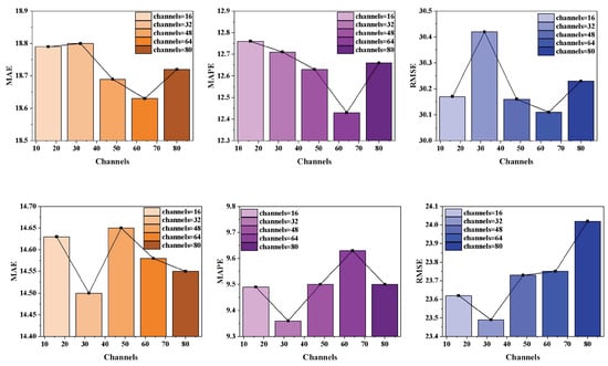
Figure 8.
Impact of feature channel count on model performance (PEMS04 (above) PEMS08 (below)).
5.6. Computation Time
Table 4 illustrates the comparison we made in this section between the ADDGCN model’s computational cost and a few baseline models on the PEMS08 dataset. The results indicate that while ADDGCN exhibits excellent performance, it does not incur excessive computational costs. Compared to other advanced baseline models like GWN and STG-NCDE, ADDGCN outperforms its counterparts while incurring much lower computational costs. This is achieved through the parallel processing of data and the lightweight nature of the model. Although SCINet and AGCRN have lower computational costs, SCINet falls short in capturing spatial correlations, and AGCRN, while adept at capturing spatial correlations, is limited in its learning of spatio-temporal information interactions. The primary source of computational cost for ADDGCN is the interaction learning process in its subsampling dynamic graph convolutional structure. The model adopts a non-autoregressive approach to parallel data processing, thereby enhancing efficiency.
Table 4.
Computational costs of various models on the PEMS08 dataset.
5.7. Industrial Significance
This paper introduces a method combining feature-enhanced down-sampling dynamic graph convolution networks with multi-head attention mechanisms (ADDGCN) for traffic flow forecast. This method is not only theoretically innovative but also of significant importance in industrial applications. Firstly, by enhancing the interaction between road network node information, the method dramatically increases traffic flow forecast accuracy. This is crucial for traffic control and urban planning in particular, as accurate traffic flow predictions can effectively guide traffic signal control and network optimization, reducing traffic congestion and improving road usage efficiency. For example, precise traffic flow predictions can help traffic managers adjust signal cycles reasonably during peak hours, alleviating the pressure at intersections, reducing vehicle queuing times, and thus enhancing urban traffic fluidity.
Secondly, improving the accuracy of traffic flow predictions also positively contributes to environmental protection. By reducing traffic congestion, we can effectively lower vehicle emissions, reducing air pollution and greenhouse gas emissions. This holds significant importance for sustainable urban development and addressing climate change. Additionally, more efficient traffic flow management can also help reduce the incidence of traffic accidents, improving road safety.
Lastly, the precision enhancement in traffic flow forecasting also shows tremendous potential in terms of adaptability for future technologies. With the advancement of autonomous driving and intelligent traffic systems, accurate traffic flow forecasting will become an indispensable part of these technologies. The approach suggested in this study offers a solid foundation for integrating these innovative technologies, heralding a more intelligent and efficient transportation future.
6. Conclusions and the Future Work
In the present study, we introduce ADDGCN, a pioneering attention-fused down-sampling dynamic spatio-temporal graph neural network model, designed for traffic forecasting tasks. Specifically, we incorporate dynamic graph convolution into the interactive learning architecture of down-sampled convolutional networks with the aim of simultaneously capturing spatio-temporal dependencies. In addition, we put forward a dynamic graph convolution network to simulate dynamic spatial correlation. The DGCN can discover invisible node relationships in road networks, thereby capturing hidden spatial relationships. Experiments on two publicly available traffic datasets indicate that ADDGCN performs better than cutting-edge baselines. Accurate traffic flow prediction is crucial for optimizing urban traffic management, reducing congestion, and enhancing road safety. It also assists individuals in planning their travel, improves the efficiency of public transportation, and provides data support for urban planning and environmental policies.
It is essential to acknowledge that traffic flow is profoundly impacted by diverse elements, including meteorological conditions and holidays. In our forthcoming research, we plan to integrate these influencing factors into the model to enhance its prediction accuracy. By considering weather-related variables and the impact of holidays and special events on traffic patterns, our models will be better suited for real-world scenarios and yield more precise forecasts. Moreover, we recognize that certain parameters in the current models are empirically defined and lack a strong theoretical foundation. To address this limitation and enhance the model’s overall performance, we intend to explore the incorporation of optimization algorithms. By employing advanced optimization techniques, we can fine-tune the model’s parameters, resulting in a more data-driven and accurate forecasting process. This approach will enable us to discover more optimal parameter settings, better capturing the complex relationship between traffic flow patterns and diverse influencing variables.
Author Contributions
Conceptualization, C.W. and Z.L.; methodology, H.W. and Z.L.; software, S.W.; validation, Z.L., H.W. and C.W.; formal analysis, S.W.; investigation, Z.L. and C.W.; resources, H.W.; data curation, C.W.; writing—original draft preparation, C.W. and Z.L.; visualization, H.W.; supervision, C.W.; project administration, C.W.; funding acquisition, H.W. All authors have read and agreed to the published version of the manuscript.
Funding
This work was supported by the 2023 Provincial Science and Technology Plan Project 2023BCB041 “Research and Application of Core Technologies for Intelligent Energy Saving in 5G Transmission Network Sites”, and 2023BAB022 “Research and Application of Cross-Road Domain Traffic Flow State Recognition and Migration Technology Based on Spatio-Temporal Data-Driven”.
Data Availability Statement
The authors approve that the data used to support the findings of this study are included in the article. The data used in the article can be downloaded from the following link: https://github.com/divanoresia/Traffic (accessed on 20 May 2022).
Conflicts of Interest
Author Siwei Wei was employed by the company CCCC Second Highway Consultants Co., Ltd. The remaining authors declare that the research was conducted in the absence of any commercial or financial relationships that could be construed as a potential conflict of interest.
References
- Xu, X.; Hu, X.; Zhao, Y.; Lü, X.; Aapaoja, A. Urban short-term traffic speed prediction with complicated information fusion on accidents. Expert Syst. Appl. 2023, 119887. [Google Scholar] [CrossRef]
- Zhao, J.; Huang, J.; Xiong, N. An effective exponential-based trust and reputation evaluation system in wireless sensor networks. IEEE Access 2019, 7, 33859–33869. [Google Scholar] [CrossRef]
- Tedjopurnomo, D.A.; Bao, Z.; Zheng, B.; Choudhury, F.M.; Qin, A.K. A survey on modern deep neural network for traffic prediction: Trends, methods and challenges. IEEE Trans. Knowl. Data Eng. 2020, 34, 1544–1561. [Google Scholar] [CrossRef]
- Lan, S.; Ma, Y.; Huang, W.; Wang, W.; Yang, H.; Li, P. Dstagnn: Dynamic spatial-temporal aware graph neural network for traffic flow forecasting. In Proceedings of the 39th International Conference on Machine Learning, Baltimore, MD, USA, 17–23 July 2022; PMLR International Conference on Machine Learning. Volume 2022, pp. 11906–11917. [Google Scholar]
- Zhang, W.; Zhu, K.; Zhang, S.; Chen, Q.; Xu, J. Dynamic graph convolutional networks based on spatiotemporal data embedding for traffic flow forecasting. Knowl. Based Syst. 2022, 250, 109028. [Google Scholar] [CrossRef]
- Yadav, P.; Sharma, S.C. A systematic review of localization in WSN: Machine learning and optimization-based approaches. Int. J. Commun. Syst. 2023, 36, e5397. [Google Scholar] [CrossRef]
- Li, S.; Wu, C.; Xiong, N. Hybrid architecture based on CNN and transformer for strip steel surface defect classification. Electronics 2022, 11, 1200. [Google Scholar] [CrossRef]
- Yu, B.; Yin, H.; Zhu, Z. Spatio-temporal graph convolutional networks: A deep learning framework for traffic forecasting. arXiv 2017, arXiv:1709.04875. [Google Scholar]
- Zhao, L.; Song, Y.; Zhang, C.; Liu, Y.; Wang, P.; Lin, T.; Deng, M.; Li, H. T-gcn: A temporal graph convolutional network for traffic prediction. IEEE Trans. Intell. Transp. Syst. 2019, 21, 3848–3858. [Google Scholar] [CrossRef]
- Li, Y.; Yu, R.; Shahabi, C.; Liu, Y. Diffusion convolutional recurrent neural network: Data-driven traffic forecasting. arXiv 2017, arXiv:1707.01926. [Google Scholar]
- Wang, X.; Ma, Y.; Wang, Y.; Jin, W.; Wang, X.; Tang, J.; Jia, C.; Yu, J. Traffic flow prediction via spatial temporal graph neural network. In Proceedings of the Web Conference, Taipei, Taiwan, 20–24 April 2020; pp. 1082–1092. [Google Scholar]
- Kopp, M.; Kreil, D.; Neun, M.; Jonietz, D.; Martin, H.; Herruzo, P.; Gruca, A.; Soleymani, A.; Wu, F.; Liu, Y. Traffic4cast at neurips 2020-yet more on the unreasonable effectiveness of gridded geo-spatial processes. In Proceedings of the PMLR NeurIPS 2020 Competition and Demonstration Track, Virtual, 6–12 December 2020; pp. 325–343. [Google Scholar]
- Song, C.; Lin, Y.; Guo, S.; Wan, H. Spatial-temporal synchronous graph convolutional networks: A new framework for spatial-temporal network data forecasting. Proc. AAAI Conf. Artif. Intell. 2020, 34, 914–921. [Google Scholar] [CrossRef]
- Bai, L.; Yao, L.; Li, C.; Wang, X.; Wang, C. Adaptive graph convolutional recurrent network for traffic forecasting. Adv. Neural Inf. Process. Syst. 2020, 33, 17804–17815. [Google Scholar]
- Li, F.; Feng, J.; Yan, H.; Jin, G.; Yang, F.; Sun, F.; Jin, D.; Li, Y. Dynamic graph convolutional recurrent network for traffic prediction: Benchmark and solution. ACM Trans. Knowl. Discov. Data 2023, 17, 1–21. [Google Scholar] [CrossRef]
- Luo, X.; Zhu, C.; Zhang, D.; Li, Q. Dynamic Graph Convolution Network with Spatio-Temporal Attention Fusion for Traffic Flow Prediction. arXiv 2023, arXiv:2302.12598. [Google Scholar]
- Zhang, Q.; Tan, M.; Li, C.; Xia, H.; Chang, W.; Li, M. Spatio-temporal residual graph convolutional network for short-term traffic flow prediction. IEEE Access 2023, 2169–3536. [Google Scholar] [CrossRef]
- Yousaf, I.; Ali, S. The COVID-19 outbreak and high frequency information transmission between major cryptocurrencies: Evidence from the VAR-DCC-GARCH approach. Borsa Istanb. Rev. 2020, 20, S1–S10. [Google Scholar] [CrossRef]
- Fan, D.; Sun, H.; Yao, J.; Zhang, K.; Yan, X.; Sun, Z. Well production forecasting based on ARIMA-LSTM model considering manual operations. Energy 2021, 220, 119708. [Google Scholar] [CrossRef]
- Dhiman, H.S.; Deb, D.; Guerrero, J.M. Hybrid machine intelligent SVR variants for wind forecasting and ramp events. Renew. Sustain. Energy Rev. 2019, 108, 369–379. [Google Scholar] [CrossRef]
- Uddin, S.; Haque, I.; Lu, H.; Moni, M.A.; Gide, E. Comparative performance analysis of K-nearest neighbour (KNN) algorithm and its different variants for disease prediction. Sci. Rep. 2022, 12, 6256. [Google Scholar] [CrossRef]
- Sagi, O.; Rokach, L. Approximating XGBoost with an interpretable decision tree. Inf. Sci. 2021, 572, 522–542. [Google Scholar] [CrossRef]
- Ma, X.; Tao, Z.; Wang, Y.; Yu, H.; Wang, Y. Long short-term memory neural network for traffic speed prediction using remote microwave sensor data. Transp. Res. Part C Emerg. Technol. 2015, 54, 187–197. [Google Scholar] [CrossRef]
- Cui, Z.; Ke, R.; Pu, Z.; Wang, Y. Stacked bidirectional and unidirectional LSTM recurrent neural network for forecasting network-wide traffic state with missing values. Transp. Res. Part C Emerg. Technol. 2020, 118, 102674. [Google Scholar] [CrossRef]
- Tian, C.; Chan, W. Spatial-temporal attention wavenet: A deep learning framework for traffic prediction considering spatial-temporal dependencies. IET Intell. Transp. Syst. 2020, 15, 549–561. [Google Scholar] [CrossRef]
- Bi, J.; Zhang, X.; Yuan, H.; Zhang, J.; Zhou, M. A hybrid prediction method for realistic network traffic with temporal convolutional network and LSTM. IEEE Trans. Autom. Sci. Eng. 2021, 19, 1869–1879. [Google Scholar] [CrossRef]
- Liu, M.; Zeng, A.; Xu, Z.; Lai, Q.; Xu, Q. Time series is a special sequence: Forecasting with sample convolution and interaction. arXiv 2021, arXiv:2106.09305. [Google Scholar]
- Zhai, L.; Yang, Y.; Song, S.; Ma, S.; Zhu, X.; Yang, F. STResNet: Covid-19 Detection by ResNet Transfer Learning and Stochastic Pooling. Phys. A Stat. Mech. Its Appl. 2021, 579, 126141. [Google Scholar] [CrossRef]
- Narmadha, S.; Vijayakumar, V. Spatio-Temporal vehicle traffic flow prediction using multivariate CNN and LSTM model. Mater. Today Proc. 2023, 81, 826–833. [Google Scholar] [CrossRef]
- Bruna, J.; Zaremba, W.; Szlam, A.; LeCun, Y. Spectral networks and deep locally connected networks on graphs. arXiv 2014, arXiv:1312.6203. [Google Scholar]
- Defferrard, M.; Bresson, X.; Vandergheynst, P. Convolutional neural networks on graphs with fast localized spectral filtering. Adv. Neural Inf. Process. Syst. 2016, 29. [Google Scholar]
- Bai, L.; Yao, L.; Kanhere, S.; Wang, X.; Sheng, Q. Stg2seq: Spatial-temporal graph to sequence model for multi-step passenger demand forecasting. arXiv 2019, arXiv:1905.10069. [Google Scholar]
- Woo, S.; Park, J.; Lee, J.Y.; Kweon, I.S. Cbam: Convolutional block attention module. In Proceedings of the European Conference on Computer Vision (ECCV), Munich, Germany, 8–14 September 2018; pp. 3–19. [Google Scholar]
- Fan, J.; Zhang, K.; Huang, Y.; Zhu, Y.; Chen, B. Parallel spatio-temporal attention-based TCN for multivariate time series prediction. Neural Comput. Appl. 2023, 35, 13109–13118. [Google Scholar] [CrossRef]
- Liu, Y.; Shao, Z.; Hoffmann, N. Global attention mechanism: Retain information to enhance channel-spatial interactions. arXiv 2021, arXiv:2112.05561. [Google Scholar]
- He, Z.; Zhao, C.; Huang, Y. Multivariate Time Series Deep Spatiotemporal Forecasting with Graph Neural Network. Appl. Sci. 2022, 12, 5731. [Google Scholar] [CrossRef]
- Yang, Z.; Li, K.; Gan, H.; Huang, Z.; Shi, M. HD-GCN: A Hybrid Diffusion Graph Convolutional Network. arXiv 2023, arXiv:2303.17966. [Google Scholar]
- Chaudhary, L.; Singh, B. Gumbel-SoftMax based graph convolution network approach for community detection. Int. J. Inf. Technol. 2023, 15, 3063–3070. [Google Scholar] [CrossRef]
- Wu, Z.; Pan, S.; Long, G.; Jiang, J.; Zhang, C. Graph wavenet for deep spatial-temporal graph modeling. arXiv 2019, arXiv:1906.00121. [Google Scholar]
- Eichenberger, C.; Neun, M.; Martin, H.; Herruzo, P.; Spanring, M.; Lu, Y.; Choi, S.; Konyakhin, V.; Lukashina, N.; Shpilman, A. Traffic4cast at neurips 2021-temporal and spatial few-shot transfer learning in gridded geo-spatial processes. In Proceedings of the NeurIPS 2021 Competitions and Demonstrations Track, Online, 6–14 December 2021; pp. 97–112. [Google Scholar]
- Liang, G.; Kintak, U.; Ning, X.; Tiwari, P.; Nowaczyk, S.; Kumar, N. Semantics-aware dynamic graph convolutional network for traffic flow forecasting. IEEE Trans. Veh. Technol. 2023, 72, 7796–7809. [Google Scholar] [CrossRef]
- Vaswani, A.; Shazeer, N.; Parmar, N.; Uszkoreit, J.; Jones, L.; Gomez, A.N.; Kaiser, L.; Polosukhin, I. Attention is all you need. Adv. Neural Inf. Process. Syst. 2017, 30, 6000–6010. [Google Scholar]
- Zheng, C.; Fan, X.; Wang, C.; Qi, J. Gman: A graph multi-attention network for traffic prediction. Proc. AAAI Conf. Artif. Intell. 2020, 34, 1234–1241. [Google Scholar] [CrossRef]
- Guo, S.; Lin, Y.; Feng, N.; Song, C.; Wan, H. Attention based spatial-temporal graph convolutional networks for traffic flow forecasting. Proc. AAAI Conf. Artif. Intell. 2019, 33, 922–929. [Google Scholar] [CrossRef]
- Chen, C.; Petty, K.; Skabardonis, A.; Varaiya, P.; Jia, Z. Freeway performance measurement system: Mining loop detector data. Transp. Res. Rec. 2001, 1748, 96–102. [Google Scholar] [CrossRef]
- Liu, A.; Zhang, Y. Spatial-temporal interactive dynamic graph convolution network for traffic forecasting. arXiv 2022, arXiv:2205.08689. [Google Scholar]
- Kang, L.; Chen, R.S.; Xiong, N.; Chen, Y.C.; Hu, Y.X.; Chen, C.M. Selecting hyper-parameters of Gaussian process regression based on non-inertial particle swarm optimization in Internet of Things. IEEE Access 2019, 7, 59504–59513. [Google Scholar] [CrossRef]
- Yu, J.; Li, Z.; Xiong, N.; Zhang, S.; Liu, A.; Vasilakos, A.V. A reliability and truth-aware based online digital data auction mechanism for cybersecurity in MCS. Future Gener. Comput. Syst. 2023, 141, 526–541. [Google Scholar] [CrossRef]
- Chicco, D.; Warrens, M.J.; Jurman, G. The coefficient of determination R-squared is more informative than SMAPE, MAE, MAPE, MSE and RMSE in regression analysis evaluation. PeerJ Comput. Sci. 2021, 7, e623. [Google Scholar] [CrossRef]
- Deng, J.; Chen, X.; Jiang, R.; Song, X.; Tsang, I.W. St-norm: Spatial and temporal normalization for multi-variate time series forecasting. In Proceedings of the 27th ACM SIGKDD Conference on Knowledge Discovery & Data Mining, Virtual Event Singapore, 14–18 August 2021; pp. 269–278. [Google Scholar]
Disclaimer/Publisher’s Note: The statements, opinions and data contained in all publications are solely those of the individual author(s) and contributor(s) and not of MDPI and/or the editor(s). MDPI and/or the editor(s) disclaim responsibility for any injury to people or property resulting from any ideas, methods, instructions or products referred to in the content. |
© 2024 by the authors. Licensee MDPI, Basel, Switzerland. This article is an open access article distributed under the terms and conditions of the Creative Commons Attribution (CC BY) license (https://creativecommons.org/licenses/by/4.0/).