
Effect of Jointed Rock Mass on Seismic Response of Metro Station Tunnel-Group Structures

1
College of Civil Engineering, Tongji University, Shanghai 200092, China
2
State Key Laboratory for Disaster Reduction in Civil Engineering, Tongji University, Shanghai 200092, China
*
Author to whom correspondence should be addressed.
Appl. Sci. 2024, 14(10), 4080; https://doi.org/10.3390/app14104080
Submission received: 19 April 2024
/
Revised: 6 May 2024
/
Accepted: 8 May 2024
/
Published: 11 May 2024
(This article belongs to the Special Issue Rock Mechanics in Geotechnical and Tunnel Engineering)
Abstract
:A jointed rock mass (JRM) is the usual case in practical engineering, which has significant effects on its mechanical performance. To clarify the difference in the seismic responses of underground structures in JRM sites or homogeneous rock mass (HRM) sites, two models were prepared to take shaking table tests in a structural laboratory. The HRM site was prepared following the similitude relations of material; meanwhile, underground structures of a metro station were embedded during the casting of the models. The JRM site and structure were made with the same material but produced random joints after the natural drying process. Different frequencies of harmonics were used to excite along the two models in the transverse or the longitudinal direction, respectively. The dynamic effect was evaluated by time-frequency and frequency-domain analyses. The test results compared with the HRM model indicated that the JRM model had a 22% reduction in the transverse fundamental frequency, but the dynamic response of the ground surface was enhanced due to the effect of the joints. Under harmonic excitations of the same intensity, the JRM model produced a greater energy response to the station structure and reduced the acceleration response of the platform in the high-frequency region. Meanwhile, the JRM model produced a peak tensile strain at the connections of the main and subsidiary structures that was 31% larger than that of the HRM model, and the range of tensile strains observed at the platform connecting the horizontal passage was 1.5 times larger than that of the HRM model.
1. Introduction
Underground structures suffer damage or even collapse not only in the site of soft soil, but within the strata of the rock mass during strong earthquakes. The investigated damage of mountain tunnels after the 1999 Chi-Chi earthquake [1] and the 2008 Wenchuan earthquake [2,3,4,5] have attracted the attention of practitioners and academics. Surveying the underground powerhouses after Wenchuan earthquake revealed a large area of cracking and spalling [6]. These investigations suggested that the damage to underground caverns was owing to the discontinuity of the rock mass [7,8,9].
Engineering geology has paid close attention to discontinuity, whether it is the fault, joint, folding, or other types of anisotropy [10]. Fractures, also called joints, are the planes along which stress has caused a partial loss of cohesion in the rock. It is a relatively smooth planar surface representing a plane of weakness (discontinuity) in the rock. Conventionally, a joint is defined as a plane where there is hardly any visible movement parallel to the surface of the joint; otherwise, it is classified as a fault. Although joints are extremely common and widespread in rocks, geologically they are still not well-studied [11]. Joints are created by stresses which may have diverse origins, such as (a) tectonic stresses related to the deformation of rocks; (b) residual stresses; (c) contraction due to shrinkage because of the desiccation of sediments; and (d) weathering. Generally, the deformation and damage of a rock mass are mainly controlled by the rock characteristics and the structure of joints [12]. Rock quality evaluation methods can be categorized into single-factor and multi-factor evaluation methods, including the elastic wave velocity method [13], rock quality designation (RQD) [14], rock mass rating (RMR) [15], Q system [16], and so on. The lower the rock quality, the denser the distribution of joints in the rock, and the higher the degree of heterogeneity of the rock mass. However, there are limited reports on the effect of rock joints on the seismic response of underground caverns.
The shaking table test, used to investigate the characteristics of underground caverns under an earthquake, is a powerful tool in revealing the dynamic interaction between rock and a structure. It is important to note that the strata–structure interaction plays a controlling role in the seismic response of underground caverns [17,18]. Chen et al. [19,20] conducted a large-scale shaking table test for a tunnel with varying stiffnesses of its linings under strong earthquakes. Zhao et al. [21,22] investigated the aseismic effect of grouting in a fault-crossing tunnel through shaking table tests, and explored the seismic mitigation performance of grouting, which reduced the acceleration response of fault-crossing tunnels. Li et al. [23,24] investigated the dynamic characteristics of a tunnel-crossing soil–rock interface using shaking table tests, and the combined effect of the soil–rock interface and the tunnel was due to the differential ground seismic response. The aforementioned studies primarily focused on a single underground cavern and assumed that the strata were a continuous medium. Experimental studies on jointed rock masses under earthquakes are rare, except for with numerical simulations [25,26,27,28].
The tunnel-group metro station is a new type of station structure form, which is characterized by a shallow burial depth, separation of the hall from the platforms, which is connected by horizontal passages and inclining shafts, and large-span column-free structures for the station hall. These structural features distinguish the tunnel-group metro station structures significantly from the frame-box metro stations in soft soil, making them more akin to underground caverns. However, they differ from the underground powerhouses of hydroelectric stations due to the high density of people and the frequent train services within the metro stations. As a novel structural form, however, there is no research on the experimental studies for tunnel-group metro station structures, and only a preliminary study using finite element method has been carried out [29].
In this study, the seismic response of the metro station tunnel-group structures with different strata characteristics was evaluated by shaking table tests. Two models, one being a homogeneous rock–station model as a reference group, and the other a jointed rock–station model as a control group, were fabricated by deriving the similitude theory. The station structures were prepared from the same plaster material. Both models were excited with the same sinusoidal waves to ensure the comparability of the results. The acceleration sensors and strain gauges were arranged at the corresponding locations of the two models. The effect of the jointed rock on the metro station tunnel-group structures was discussed by quantifying the rock–structure interaction through time-frequency and frequency-domain analyses, such as transfer function, power spectral density, and Arias Intensity.
2. Models: Design and Fabrication
2.1. Tunnel-Group Structures
The test was carried out using the shaking table from the State Key Laboratory of Tongji University with a size of 4 m × 4 m and a maximum load capacity of 25 tons. Dynamic interaction of the rock and structure was concentrated on the tunnel-group metro station. Specific scaled structures included the main structures (one hall tunnel and two platform tunnels) and the subsidiary structures (one horizontal passage connecting two platform tunnels and one inclining shaft connecting station hall and horizontal passage). Non-structural elements of the station, such as air ducts, work shafts, and metro tunnels, were ignored. By considering the confinements from the size and capability of shaking table, dimensions of ground and station to be modeled, as well as the selection of model materials, the geometric similitude ratio (model to prototype) of the model was determined as 1:30. The actual dimensions of the model station could be calculated, and Figure 1 illustrates the geometric dimensions of each part of the model station.
2.2. Similitude Relations
The model systems were rigorously designed and calculated using similitude theory, and prototype using the same set of similitude relations for strata and structures to ensure representative model testing. Deriving the similitude relations using dimensional analysis [30], the following equation could be obtained:
where , , , and were the similitude ratios of acceleration, Young’s modulus, geometry, and density, respectively. The similitude ratios for geometry, Young’s modulus, and acceleration were determined to be 1/30, 1/100, and 1/1, respectively, based on the capacity of shaking table. Other similitude relations were derived using Equation (1), as shown in Table 1.
2.3. Materials as Structural Lining and Rock Mass
The selection of foam concrete as the material simulating the rock was based on its mechanical properties and low density [19,20,21,22]. After extensive testing to evaluate the performance at different mix ratios, a water-to-foam volume ratio of 1:4 and a water-to-cement mass ratio of 1:2.25 were selected. Meanwhile, light aggregate plaster, consisting of a 1:0.1:1.6 mass ratio of plaster, diatomite, and water, was chosen to simulate the concrete of the lining. The mechanical properties of the prototype, the target values derived from similitude relations, and the test values are presented in Table 2. Due to the material limitations, we tried to control the test density and elastic modulus of the model rock and lining to be close to the target values, and ultimately the error was controlled to be within the range of 5%. This indicates that it is difficult to strictly satisfy the target values for the test values of density and modulus, which is consistent with the model material selection in the references [9,20,21].
2.4. Model Fabrication
The preparation of the model mainly included four steps: pouring of the light aggregate plaster lining, maintenance indoors, assembly of the lining, and pouring the foam concrete, and Figure 2 presents the construction process of the models. Foam concrete was molded in one pour for HRM model and four pours for JRM model. Because of the presence of construction joints at the poured layering and the drying shrinkage of foam concrete, artificial rock joints and discontinuous planes were created through a period of natural curing.
A series of tests was conducted using a six-degrees-of-freedom shaking table system at Tongji University, which is 4.0 m long and 4.0 m wide with a load capacity of 25 tons. The outer contour of the whole model was 3.0 m long in the x-direction, 3.0 m wide in the y-direction, and 2.0 m high in the z-direction. Figure 3 illustrates the complete test models, Figure 3a is an actual picture of HRM model, and Figure 3b is a sketch of the joints and discontinuous planes of JRM model.
Wu et al. [31,32] combined the strain energy theories of continuum and fracture mechanics, the elastic stress–strain relationship of the jointed rock mass was proposed, and its elastic modulus was derived. The ratio of elastic modulus of jointed rock to that of an intact rock was defined, and when the joints were in compression (σ ≤ 0), the formula was as follows:
where , , and is Poisson’s ratio of the medium around the joints, and the Poisson’s ratio of the model rock is 0.3; is the inter-angle between the shear stress and the loading plane; m is the number of joint sets; λ and are the normal density and average radius of the joint sets, respectively; and h is the residual shear stress ratio, since the medium and roughness around the joints are the same, and it is assumed to be 0.9 for all cases.
The joints on the model surface were categorized Into the left side (ml), the front face (mf), the right side (mr), the back face (mb), and the top face (mt). Along the loading directions, the joints were divided into two sets: the side joint sets, consisting of left side ml and right side mr (in the x-direction); and the face joint sets, consisting of front face mf, back face mb, and top face mt (in the y-direction). Under transverse (x-direction) loading, the angle between the side joint sets and the loading plane was 90°, and the angle between the face joint sets and the loading plane was 15°. Similarly, under longitudinal (y-direction) loading, the angle between the side joint sets and the loading plane was 90°, and the angle between the face joint sets and the loading plane was 75°. The parameters of joints are shown in Table 3.
According to Equation (2), the values of in the transverse and longitudinal directions can be estimated to be approximately 0.82 and 0.95, respectively. It was evident that the distribution of joints has a significant impact on the transverse stiffness of the JRM model, while the effect on longitudinal stiffness was small.
3. Test Setup
3.1. Instrumentation
The locations of these instruments were all based on numerical simulations using finite element method [29], as shown in Figure 4.
For comparison between the two models, sensors were arranged at identical locations. As shown in Figure 4a, an accelerometer AS1 was placed at the top center of the model and accelerometer AS2 was placed at the top boundary of the model, which were allowed for the calculation of boundary effects and the influence of underground metro stations on dynamic responses of the ground surface. Accelerometers (AS0, AS3, and AS2) were arranged along the vertical direction of the model boundary to analyze the amplification effect in the vertical direction of the surrounding rock.
Accelerometers A1 to A8 were arranged inside the main structure of the station, and there were two observation sections in the hall; A1 (vault) and A2 (inverted arch) were opening section, and A3 and A4 were normal section. Similarly, accelerometers on the platform were arranged, with accelerometers in the normal section numbered A5 and A6, and accelerometers in the opening section numbered A7 and A8, as shown in Figure 4b. By recording acceleration responses, differences in acceleration between the opening and normal sections could be compared.
As shown in Figure 4c, strain gauges were arranged to study the dynamic tensile strain and spatial distribution of the station, because the connections between the main structures and the subsidiary structures are locations of stress concentration. VL represents the lower part of the inclined shaft, and HR represents the right part of the horizontal passage. Bidirectional strain gauges were placed on the vault (V1 and H1), spandrel (V2 and H2), arch footing (V3 and H3), and arch bottom (V4 and H4) for each section. Additionally, strain gauges (H5, H6, H7, and H8) were longitudinally arranged along the right platform at the same height as the vault (H1), with a spacing of 260 mm between H5~H8, to calculate the range of tensile strains at the platform connecting the horizontal passage.
3.2. Inputs of Harmonic Excitation
Actual earthquakes can be decomposed into the superposition of multiple harmonics, and a single harmonic has a simple mathematical description and clear frequency characteristics, which facilitates experimental analysis of the dynamic response of structures. In contrast, actual seismic records usually show complex waveforms with long duration and poor repeatability. In the test, the sinusoidal accelerations with frequencies of 12, 17, 19, 21, and 23 Hz were used as excitation seismic waves according to the frequency similitude ratio 5.48 (Section 2.2), since the HRM model’s estimated dominant frequency was 20 Hz [26]. The series of seismic excitations is shown in Figure 5.
Before applying the harmonic excitations, a white noise excitation (WN1) was used to investigate the inherent dynamic properties of the models. The peak value of the white noise excitation was set at 0.05 g, aiming to conduct a “zero test” [33]. Each excitation phase comprised conditions with transverse excitation (x-direction) and longitudinal excitation (y-direction). A comprehensive list of all test cases can be found in Table 4. The two models adopted identical test cases.
4. Comparison between Two Models
The dynamic responses of the sites and the station structures were presented and analyzed, with a particular discussion of the spectral differences between the two model sites, the acceleration response, the energy response of the main structures, the peak tensile strains at the structural connections, and the range of tensile strains at the platform connecting the horizontal passage. Unless otherwise stated, the results are shown at the model scale.
4.1. Acceleration Responses of the Sites
4.1.1. Acceleration Time Histories of Ground Surfaces
Two acceleration measurement points, AS1 and AS2, at the top of the models were selected to analyze the acceleration response under different harmonic excitations. Figure 6 shows the acceleration time histories under transverse excitation and longitudinal excitation for a specific time period, and it can be found that the waveforms of the two measurement points are in good agreement. The acceleration error is defined as the difference between the peak acceleration of AS1 and AS2.
By calculation, the acceleration errors were within 3% for the HRM model and 10% for the JRM model under a transverse excitation, and the JRM model also showed good agreement at the excitation frequencies of 21 Hz and 23 Hz.
Under longitudinal excitation, the acceleration errors were within 5% for the HRM model and 12% for the JRM model. Because there are many joint sets in the JRM model compared to the HRM model, under harmonic excitation, the seismic motions were reflected and refracted between the joint sets, which increased the dynamic response at the model boundary, resulting in a more pronounced boundary effect in the JRM model than in the HRM model.
With the above analysis, the boundary effects of the rock models were small and the AS2 measurement point can be considered as in “free field”, which serves as the basis for the power spectral density analysis in Section 4.2.2.
4.1.2. Acceleration Amplification Factors along the Rock Height
The variation in the peak acceleration along the rock height can be expressed using the acceleration amplification factor (AAF). It is defined as the ratio of the peak acceleration at the measurement points to the peak acceleration input from the shaking table [34].
In order to evaluate the acceleration amplification effect of the rock models along the vertical direction, three measurement points were selected: AS0, AS3, and AS2. The AAF under different frequency excitations was compared, as shown in Figure 7.
Overall, the acceleration increased gradually from bottom to top and reached the maximum at the ground surface. Under the transverse excitation, the HRM model exhibited an increasing acceleration amplification effect with frequency, and reached the maximum value of 4.1 at 23 Hz of the input case. The AAF of the JRM model showed a tendency of increasing and then decreasing, and reached the maximum value of 4.0 at 17 Hz of the input case.
Under longitudinal excitation, the AAF of the HRM model reached the peak at 21 Hz of the input case, with a maximum value of 2.9. The AAF of the JRM model reached the peak at 19 Hz of the input case, with a maximum value of 2.8.
The difference between the amplification effect of the JRM model and the HRM model was due to the greater effect of the joints on the transverse modulus of the JRM model, which resulted in the transverse fundamental frequency of the JRM model being much smaller than that of the HRM model, causing the JRM model to reach the peak at 17 Hz of the input case. The smaller effect of the joints on the longitudinal modulus resulted in the longitudinal fundamental frequency of the JRM model being slightly smaller than that of the HRM model, causing the JRM model to reach the peak at 19 Hz of the input case. This was analyzed in Section 2.4 by applying the elastic modulus equation for a jointed rock mass, and was verified by the white noise transfer function in Section 4.2.1.
In summary, the seismic responses of the rock models showed an obvious amplification effect, which was correlated with the excitation frequency. Meanwhile, the maximum acceleration amplification factors of the two models were similar, but the peak response frequency of the JRM model was lower than that of the HRM model, which is attributed to the reduction of the model stiffness due to the joints and discontinuity planes in the JRM model.
4.2. Frequency Response of the Models
4.2.1. Transfer Function
In order to study the dynamic characteristics of different sites, the transfer function (TF) was chosen as an evaluation indicator [35]. An attempt was made to compare the dynamic characteristics of different regions of the models in the frequency domain. The transfer function is defined as follows: the ratio of the Laplace transform of the output signal to the Laplace transform of the input signal:
where and representing the Laplace transforms of the input and output signals, respectively.
To assess the spectral characteristics of different sites, the transfer functions under white noise excitations (WN1) at AS1, AS2, and A3 were compared. Considering that the ground surface AAF under sinusoidal excitation theoretically approximates the magnitude of the transfer functions under white noise excitation, the AAF at AS1 and AS2 was also compared, as shown in Figure 8. It can be observed that for the HRM model, the transverse fundamental frequency in all three areas was 22.1 Hz, and the longitudinal fundamental frequency was 20.3 Hz; for the JRM model, the transverse fundamental frequency in all three areas was 17.3 Hz, and the longitudinal main frequency was 20.2 Hz. The difference in the fundamental frequency responses of the two models is consistent with the conclusions about the elastic modulus of the models presented in Section 2.4. The following five points can be summarized.
- (1)
- The AAF at AS1 and AS2 fell within the range of the ground surface transfer functions, indicating the reliability of the similitude design and model fabrication, ensuring the comparability between the two models.
- (2)
- The spectral characteristics of the structures were controlled by the sites. This explains the observations in Figure 7a, where the excitation frequency of 23 Hz of the input case was close to the transverse fundamental frequency of 22.1 Hz for the HRM model; hence, the amplification effect was not significantly reduced.
- (3)
- It is worth noting that the presence of the station structure resulted in a slightly smaller amplitude of the ground surface transfer function (AS1) than the free field (AS2), which may be due to the station structures absorbing more input energy, leading to a smaller response at the top of the models. This coincides with the conclusion of the power spectral density analysis in Section 4.4.2 and is also verified in reference [35] regarding the effect of underground structures on the surface.
- (4)
- Compared to the HRM model, the JRM model had a significantly lower transverse fundamental frequency, while the longitudinal fundamental frequency remained essentially unchanged. This suggests that the transverse stiffness of the JRM model was reduced due to the influence of joints and discontinuous planes, while the longitudinal stiffness remained unchanged. The discontinuous plane at the top face of the JRM model in Figure 3b might be the primary reason for this. Meanwhile, the transverse fundamental frequency magnitude of the JRM model was 1.51 times that of the HRM model, possibly due to reflections and refractions of seismic waves caused by joints and discontinuous planes, enhancing the dynamic response at the ground surface.
- (5)
- Comparing the ground surface AS1 and AS2 within the same model, their transverse transfer function curves essentially coincided, with the fundamental frequency and magnitude being nearly identical, further proving that the AS2 location represents a “free field”. Similarly, the longitudinal transfer functions of AS1 and AS2 followed the same pattern.
In summary, the differences in the amplitude and fundamental frequency of the transfer functions indicate that the two models exhibit distinct seismic response characteristics, and the two types of site have different rock–structure dynamic interactions.
4.2.2. Acceleration Power Spectral Density
Since the harmonic frequency has a single characteristic, the test results of the harmonic excitations are easy to analyze the spectrum. The acceleration power spectral density (PSD) was used as an evaluation indicator [36], which defines the energy distribution of seismic excitation at different frequencies. The PSD at the top of the models (AS1 and AS2) and at the bottom of the models (AS0) are shown in Figure 9. The Welch method [31] was used to calculate the PSD at the measurement points. Overall, the PSD of AS0 at the bottom of the models decreased as the harmonic frequency increased. However, the PSD at the top of the models exhibited a different pattern.
Under transverse excitation, the maximum amplitudes of the HRM model and the JRM model appeared at 12 Hz and 17 Hz, respectively, and the maximum amplitude of the JRM model was 1.21 times that of the HRM model. Under longitudinal excitation, the maximum amplitude of both models occurred at 19 Hz, and the maximum amplitude of the JRM model was 1.44 times that of the HRM model. This indicates that the amplification effect of the model rocks is related to the direction of excitations, and the jointed rock produces a more significant amplification response under the same excitations. In addition, the PSD of AS1 was mostly smaller than that of AS2, which may be due to the effect of the buried metro station.
To investigate the effect of the station structure on the ground dynamic response, the ratio of PSD at the top and bottom of the model is shown in Figure 10. The variation in the PSD ratios with frequency is consistent with the variation rule of the AAF in Section 4.1.2, i.e., the peaks of the HRM model and the JRM model occurred at 23 Hz and 17 Hz for transverse excitation, and at 21 Hz and 19 Hz for longitudinal excitation, respectively. Meanwhile, the PSD ratios of the rock–structure field (AS1/AS0) were smaller than that of the “free field” (AS2/AS0). When the difference between the PSD ratios of the rock–structure and the “free field” was larger, it indicated that more input energy was consumed by the buried station, especially when the input frequency was close to the fundamental of the models. The variation in the PSD amplitude of AS0 with the frequency and the effect of the underground structure on the PSD ratio of the surface were in accordance with the conclusions of reference [37].
4.3. Acceleration Responses of the Main Structures
4.3.1. Acceleration Time Histories of the Main Structures
Under harmonic excitation, a comparison of the horizontal acceleration time histories of the station structures for the two models is presented in Figure 11, showcasing representative frequencies of 12 Hz and 21 Hz. It is observed that at lower input frequencies, the acceleration time histories at the same measurement points of the two models are quite similar; however, as the input frequency increases, significant differences in the peak acceleration at the measurement points between the two models emerge. Overall, the acceleration response at the vault is larger than that at the arch bottom, and the acceleration response at the station hall is larger than that at the platform. Meanwhile, the lining acceleration amplitudes of the two models have different patterns of variation depending on the frequency and direction of excitation, which is further explained in Section 4.3.2.
4.3.2. Acceleration Amplification Factors
The frequency response factor (FRF) is defined as the ratio of the input frequency to the fundamental frequency of the model, and is expressed by the following equations:
where is the frequency of harmonic, corresponds to 22.1 Hz and 17.3 Hz for the HRM model and the JRM model, respectively; while corresponds to 20.3 Hz and 20.2 Hz for the HRM model and the JRM model, respectively.
Acceleration response–frequency curves of the main structures are shown in Figure 12. When β approaches 1, it means that the input frequency is close to the fundamental frequency of the models, and then the AAF reaches its peak, i.e., the acceleration amplification effect of the structure is the most significant. The differences in the AAF at the measurement points are compared in Table 5.
Overall, the AAFs at the vault are all larger than those at the arch bottom, indicating a significant amplification effect at the vault. Under harmonic transverse excitation, the amplification factors of the hall opening section were larger than that of the normal section in both models, i.e., A1 and A3 and A2 and A4 were compared to show that there is an amplification effect at the hall opening section, and the comparison through A5 and A7 and A6 and A8 showed that there was no amplification effect in the platform opening sections. Under harmonic longitudinal excitation, there was no amplification effect in the opening section of the HRM model as both A1/A3 and A2/A4 were less than 1.0; however, in the JRM model, A2/A4 = 1.18, so there was an amplification effect in the opening section of its hall. It can also be observed that the amplification factors at the platform measurement points of the JRM model were less than 1.0 in the high-frequency region, indicating that there was a phenomenon of acceleration reduction, which may be due to the fact that the joint sets consume more input energy under high-frequency excitation, reducing the seismic response of the station structure.
4.3.3. Arias Intensity
In order to further analyze the dynamic response of the lining, the Arias intensity (IA) was introduced, which can quantify the magnitude of the energy of earthquakes and characterize the situation of potential structural hazards induced by earthquakes [14]. The simplified expression is as follows:
where a(t) is the earthquake acceleration time history, g is the acceleration of gravity, and Td is the total duration of the earthquake acceleration record.
The lining measurement points were compared with the input seismic waves of the shaking table to obtain the IA and the energy amplification factor (EAF) (EAF = IA of the acceleration measurement points/IA of the shaking table). Energy response–frequency curves of the main structures are shown in Figure 13.
It can be observed that the variation rule of the EAF of the lining was very similar to that of the AAF, and the EAF reached the peak value when β was close to 1. Compared with the AAF, the EAF of the hall vault (A1 and A3) in the JRM model was more significant near the fundamental frequency of the rocks, and the maximum values of the EAF under the transverse and the longitudinal excitation were 7.1 and 9.1, respectively. This indicates that the force of the JRM site produced a greater energy response to the station structure, and the station structure was more prone to damage.
In addition, the energy response intensity under transverse excitation was greater than that under longitudinal excitation in the HRM model, while the energy response intensity under longitudinal excitation was greater than that under transverse excitation in the JRM model, which is consistent with the previous analysis.
4.4. Dynamic Strain of the Station Structures
4.4.1. Dynamic Strain Time Histories at Structural Connections
We compared the strain time histories at corresponding measurement points on the VL and HR sections, as shown in Figure 14, with representative frequencies of 17 Hz and 19 Hz displayed. Overall, the dynamic tensile strains at the vault and arch bottom were relatively small, with the JRM model exhibiting greater dynamic tensile strains than the HRM model at the corresponding measurement points. Under transverse excitation, the maximum tensile strains of the VL section appeared in the spandrel V2, while under longitudinal excitation, the maximum tensile strain on the HR section occurred at the arch footing H3.
4.4.2. Peak Tensile Strain at Structural Connections
The peak tensile strains of the VL and HR sections are shown in Figure 15. It can be observed that the variation pattern of peak tensile strain is consistent with that of the AAF and the EAF, which again verifies that the dynamic response of the structure is controlled by the sites.
Under harmonic transverse excitation, the VL section in HRM model experienced greater forces, and the maximum tensile strain occurred in the spandrel, with a value of 42 με. In the JRM model, the VL section also experienced greater force, with the maximum value still at the spandrel, valued at 46 με.
Under harmonic longitudinal excitation, the situation was reversed. Both models experienced greater forces on the HR section. The maximum tensile strain occurred in the arch footing, with a value of 36 με for the HRM model and 55 με for the JRM model, which are much smaller than the cracking strain of reinforced concrete of 320 με. On the one hand, it shows that the connections between the main structures and subsidiary structures are the concentration points of forces in the tunnel-group metro station during earthquakes. On the other hand, it validates that HRM model exhibiting a greater strain response under transverse excitation, while the JRM model showed a greater strain response under longitudinal excitation. Meanwhile, the maximum tensile strain of the JRM model increased by 31% compared to the HRM model.
4.4.3. Range of Tensile Strains at the Platform Connecting the Horizontal Passage
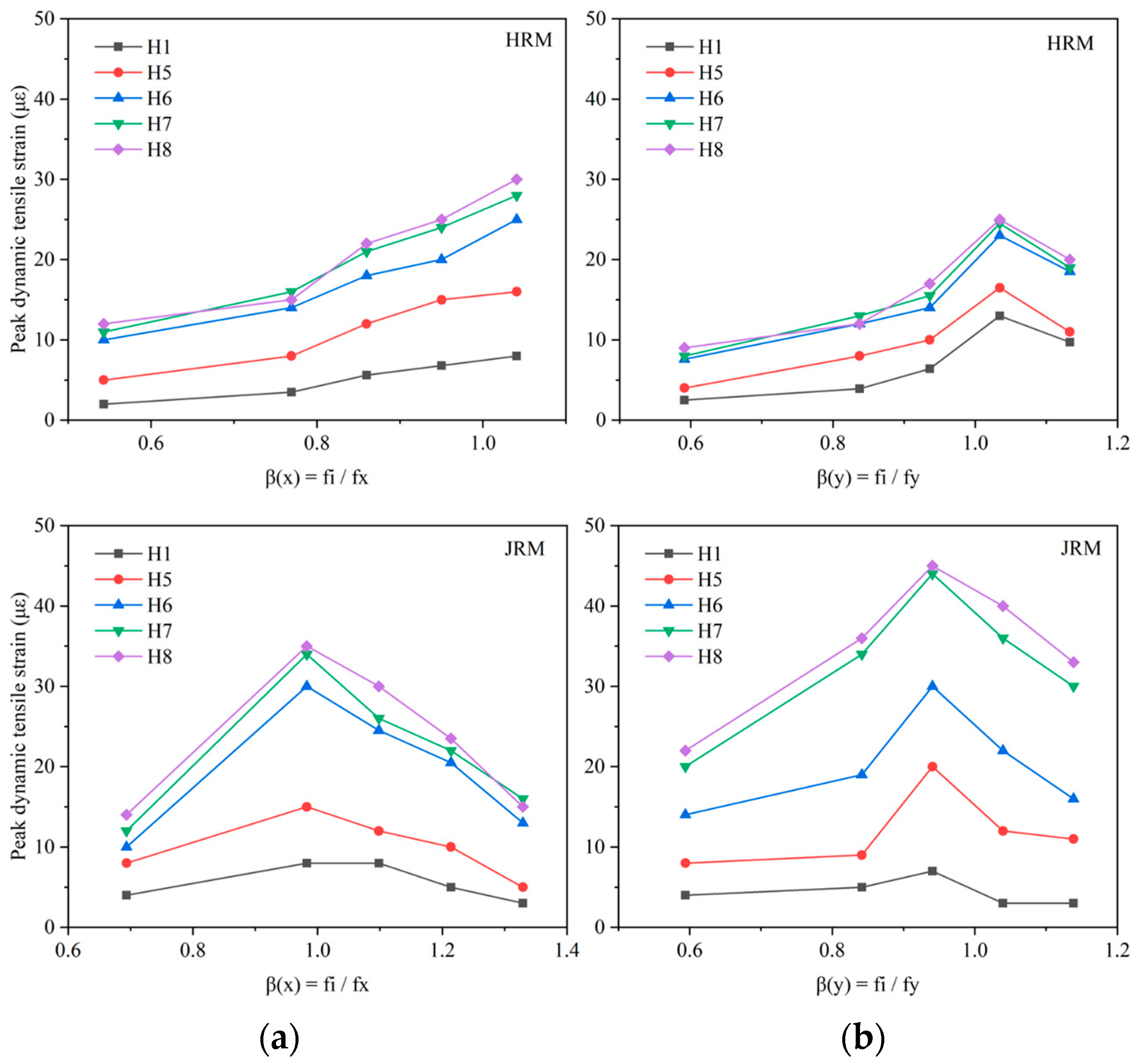
The frequency response curves of peak tensile strains at the same height of the platform are shown in Figure 16. The peak tensile strains became larger as the measurement points moved farther away from the horizontal passage, which is due to the horizontal passage increasing the stiffness of the lining cross-section. The maximum tensile strains at H7 and H8, which are the farthest away from the horizontal passage, were basically close to each other, indicating that the dynamic response of the platform at this location is almost unaffected by the horizontal passage. According to the comparison of the peak strains at H6 with those at H7 and H8, the range of tensile strains at the platform connecting the horizontal passage under different excitation directions can be discerned.
Under transverse excitation, the peak strains at H6 for both the models were similar to those at H7 and H8, which were less affected by the horizontal passage, and the range of tensile strains at the platform connecting the horizontal passage was about twice its span of the horizontal passage.
Under longitudinal excitation, the HRM model followed the aforementioned pattern, while the peak strain at H6 for the JRM model was only two-thirds of that at H7 and H8, showing that its platform was still affected by the horizontal passage. Thus, for the JRM model, the range of tensile strains at the platform connecting the horizontal passage was about three times its span of the horizontal passage. This again demonstrates that the JRM model has a greater seismic response under longitudinal excitation.
5. Conclusions
Through the large-scale shaking table tests, a detailed comparison of the seismic response between the jointed rock mass–station model and the homogeneous rock mass–station model was conducted. Different frequencies of harmonics were used to excite along the transverse and longitudinal directions, respectively.
The following conclusions could be drawn.
- (1)
- The adverse effects of joints and discontinuities on the site were quantified according to the elastic modulus formula of the jointed rock mass. Compared to the HRM model, the JRM model had a 22% reduction in the transverse fundamental frequency due to the effect of joints, but enhanced the dynamic response of the ground surface.
- (2)
- The presence of buried metro stations reduces the dynamic response of the ground surface. The closer the input frequency is to the model’s fundamental frequency, the more energy the underground structure consumes.
- (3)
- The HRM model and the JRM model produce different rock–structure dynamic interactions. Under a harmonic excitation of the same intensity, the JRM model produced a greater energy response to the station structure and reduced the acceleration response of the platform in the high-frequency region. The HRM model exhibited a greater seismic response under transverse excitation, while the JRM model showed a greater seismic response under longitudinal excitation.
- (4)
- For both models, greater tensile strains were generated at the connections of the main and subsidiary structures. The JRM model produced a peak tensile strain at the connections of the main and subsidiary structures that was 31% larger than that of the HRM model. In the JRM model, the range of tensile strains at the platform connecting the horizontal passage was approximately three times its span of the horizontal passage. Meanwhile, in the HRM model, the range of tensile strains at the platform connecting the horizontal passage was about twice its span of the horizontal passage.
This paper provides experimental insights into the seismic response of the jointed rock mass site–station structure. However, many factors may affect the dynamic response of jointed rock mass sites, including the inclination of the joints, the scale effect of the rock mass, and the oblique incidence of seismic waves. After being calibrated with the experiments, further numerical analysis is needed to reveal the seismic response of a jointed rock mass.
Author Contributions
Conceptualization, R.L. and Y.Y.; methodology, Y.Y.; software, R.L.; validation, Y.Y. and R.L.; formal analysis, R.L.; investigation, R.L.; resources, Y.Y.; data curation, R.L.; writing—original draft preparation, R.L.; writing—review and editing, Y.Y.; supervision, Y.Y.; funding acquisition, Y.Y. All authors have read and agreed to the published version of the manuscript.
Funding
This research was funded by the National Natural Science Foundation of China (grant number 52061135112).
Institutional Review Board Statement
Not applicable.
Informed Consent Statement
Not applicable.
Data Availability Statement
The original contributions presented in the study are included in the article, further inquiries can be directed to the corresponding author.
Conflicts of Interest
The authors declare no conflicts of interest.
Abbreviations
The following abbreviations are used in this manuscript:
| JRM | Jointed rock mass |
| HRM | Homogeneous rock mass |
| AAF | Acceleration amplification factor |
| PSD | Power spectral density |
| FRF | Frequency response factor |
| IA | Arias intensity |
| EAF | Energy amplification factor |
| Symbols | |
| similitude ratios of acceleration | |
| similitude ratios of Young’s modulus | |
| similitude ratios of geometry | |
| similitude ratios of density | |
| inter-angle between the shear stress and the loading plane | |
| m | number of joint sets |
| λ | normal density |
| average radius of the joint sets | |
| h | residual shear stress ratio |
| ratio of the input frequency to the fundamental frequency of the model | |
| a(t) | earthquake acceleration time history |
| με | micro strain |
References
- Wang, W.L.; Wang, T.T.; Su, J.J.; Lin, C.H.; Seng, C.R.; Huang, T.H. Assessment of damage in mountain tunnels due to the Taiwan Chi-Chi Earthquake. Tunn. Undergr. Space Technol. 2001, 16, 133–150. [Google Scholar] [CrossRef]
- Wang, Z.; Gao, B.; Jiang, Y.; Yuan, S. Investigation and assessment on mountain tunnels and geotechnical damage after the Wenchuan earthquake. Sci. China Ser. E-Technol. Sci. 2009, 52, 546–558. [Google Scholar] [CrossRef]
- Shen, Y.; Gao, B.; Yang, X.; Tao, S. Seismic damage mechanism and dynamic deformation characteristic analysis of mountain tunnel after Wenchuan earthquake. Eng. Geol. 2014, 180, 85–98. [Google Scholar] [CrossRef]
- Yu, H.T.; Chen, J.T.; Yuan, Y.; Zhao, X. Seismic damage of mountain tunnels during the 5.12 Wenchuan earthquake. J. Mt. Sci. 2016, 13, 1958–1972. [Google Scholar] [CrossRef]
- Yu, H.; Chen, J.; Bobet, A.; Yuan, Y. Damage observation and assessment of the Longxi tunnel during the Wenchuan earthquake. Tunn. Undergr. Space Technol. 2016, 54, 102–116. [Google Scholar] [CrossRef]
- Wang, X.; Chen, J.; Xiao, M. Seismic damage assessment and mechanism analysis of underground powerhouse of the Yingxiuwan Hydropower Station under the Wenchuan earthquake. Soil. Dyn. Earthq. Eng. 2018, 113, 112–123. [Google Scholar] [CrossRef]
- Ardeshiri-Lajimi, S.; Yazdani, M.; Langroudi, A.A. Control of fault lay-out on seismic design of large underground caverns. Tunn. Undergr. Space Technol. 2015, 50, 305–316. [Google Scholar] [CrossRef]
- Wang, X.; Xiong, Q.; Zhou, H.; Chen, J.; Xiao, M. Three-dimensional (3D) dynamic finite element modeling of the effects of a geological fault on the seismic response of underground caverns. Tunn. Undergr. Space Technol. 2020, 96, 103210. [Google Scholar] [CrossRef]
- Shen, Y.S.; Wang, Z.Z.; Yu, J.; Zhang, X.; Gao, B. Shaking table test on flexible joints of mountain tunnels passing through normal fault. Tunn. Undergr. Space Technol. 2020, 98, 103299. [Google Scholar] [CrossRef]
- Gudmundsson, A. The propagation paths of fluid-driven fractures in layered and faulted rocks. Geol. Mag. 2022, 159, 1978–2001. [Google Scholar] [CrossRef]
- Price, N.J.; Cosgrove, J.W. Analysis of Geological Structures; Cambridge University Press: Cambridge, UK, 1990. [Google Scholar]
- Singhal, B.B.S.; Gupta, R.P. Applied Hydrogeology of Fractured Rocks; Springer Science & Business Media: Berlin/Heidelberg, Germany, 2010. [Google Scholar] [CrossRef]
- Byun, J.H.; Lee, J.S.; Park, K.; Yoon, H.K. Prediction of crack density in porous-cracked rocks from elastic wave velocities. J. Appl. Geophys. 2015, 115, 110–119. [Google Scholar] [CrossRef]
- Deere, D. The rock quality designation (RQD) index in practice. In Rock Classification Systems for Engineering Purposes; ASTM International: Cincinnati, OH, USA, 1988. [Google Scholar] [CrossRef]
- Zhang, Q.; Huang, X.; Zhu, H.; Li, J. Quantitative assessments of the correlations between rock mass rating (RMR) and geological strength index (GSI). Tunn. Undergr. Space Technol. 2019, 83, 73–81. [Google Scholar] [CrossRef]
- Palmstrom, A.; Broch, E. Use and misuse of rock mass classification systems with particular reference to the Q-system. Tunn. Undergr. Space Technol. 2006, 21, 575–593. [Google Scholar] [CrossRef]
- Kausel, E. Early history of soil–structure interaction. Soil. Dyn. Earthq. Eng. 2010, 30, 822–832. [Google Scholar] [CrossRef]
- Anand, V.; Kumar, S.S. Seismic soil-structure interaction: A state-of-the-art review. Structures 2018, 16, 317–326. [Google Scholar] [CrossRef]
- Chen, J.; Yuan, Y.; Yu, H. Dynamic response of segmental lining tunnel. Geotech. Test. J. 2020, 43, 660–682. [Google Scholar] [CrossRef]
- Chen, J.; Yu, H.; Bobet, A.; Yuan, Y. Shaking table tests of transition tunnel connecting TBM and drill-and-blast tunnels. Tunn. Undergr. Space Technol. 2020, 96, 103197. [Google Scholar] [CrossRef]
- Zhao, X.; Li, R.; Yuan, Y.; Yu, H.; Zhao, M.; Huang, J. Shaking table tests on fault-crossing tunnels and aseismic effect of grouting. Tunn. Undergr. Space Technol. 2022, 125, 104511. [Google Scholar] [CrossRef]
- Li, R.; Yuan, Y.; Zhao, X.; Bilotta, E.; Huang, J. Local Site Effect of Fault Site and Its Impact on Seismic Response of Fault-Crossing Tunnel. J. Earthq. Eng. 2024, 1–19. [Google Scholar] [CrossRef]
- Li, S.; Cudmani, R.; Xiao, M.; Guo, Z.; Yuan, Y. Ground motion amplification pattern with TBM tunnels crossing soil-rock interface: Shaking table test. Undergr. Space 2023, 12, 202–217. [Google Scholar] [CrossRef]
- Yuan, Y.; Li, S.; Yu, H.; Xiao, M.; Li, R.; Li, R. Local site effect of soil-rock ground: 1-g shaking table test. Bull. Earthq. Eng. 2023, 21, 3251–3272. [Google Scholar] [CrossRef]
- Yoo, J.K.; Park, J.S.; Park, D.; Lee, S.W. Seismic response of circular tunnels in jointed rock. KSCE J. Civ. Eng. 2018, 22, 1121–1129. [Google Scholar] [CrossRef]
- Varma, M.; Maji, V.B.; Boominathan, A. Numerical modeling of a tunnel in jointed rocks subjected to seismic loading. Undergr. Space 2019, 4, 133–146. [Google Scholar] [CrossRef]
- Huang, J.; Zhao, M.; Xu, C.; Du, X.; Jin, L.; Zhao, X. Seismic stability of jointed rock slopes under obliquely incident earthquake waves. Earthq. Eng. Eng. Vib. 2018, 17, 527–539. [Google Scholar] [CrossRef]
- Ghosh, A.; Hsiung, S.M.; Chowdhury, A.H. Seismic Response of Rock Joints and Jointed Rock Mass: Center for Nuclear Waste Regulatory Analysis; NUREG/CR-6388 CNRWA 95-013; Engineering, Environmental Science, Geology: College Station, TX, USA, 1996. [Google Scholar]
- Li, R.; Yuan, Y. Seismic Response of Tunnel-group Metro Station in a Rock Site. In Civil-Comp Conferences, Proceedings of the Seventeenth International Conference on Civil, Structural and Environmental Engineering Computing, Pécs, Hungary, 28–31 August 2023; Civil-Comp Press: Edinburgh, UK, 2023. [Google Scholar]
- Yan, X.; Yu, H.; Yuan, Y.; Yuan, J. Multi-point shaking table test of the free field under non-uniform earthquake excitation. Soils Found. 2015, 55, 985–1000. [Google Scholar] [CrossRef]
- Wu, F.; Deng, Y.; Wu, J.; Li, B.; Sha, P.; Guan, S.; Zhang, K.; He, K.; Liu, H.; Qiu, S. Stress–strain relationship in elastic stage of fractured rock mass. Eng. Geol. 2020, 268, 105498. [Google Scholar] [CrossRef]
- Wu, F.Q.; Wang, S.J. A stress–strain relation for jointed rock masses. Int. J. Rock Mech. Min. 2001, 38, 591–598. [Google Scholar] [CrossRef]
- Brennan, A.J.; Thusyanthan, N.I.; Madabhushi, S.P. Evaluation of shear modulus and damping in dynamic centrifuge tests. J. Geotech. Geoenviron. 2005, 131, 1488–1497. [Google Scholar] [CrossRef]
- Zhang, J.; Yuan, Y.; Yu, H. Shaking table tests on discrepant responses of shaft-tunnel junction in soft soil under transverse excitations. Soil Dyn. Earthq. Eng. 2019, 120, 345–359. [Google Scholar] [CrossRef]
- Yuan, Y.; Yang, Y.; Zhang, S.; Yu, H.; Sun, J. A benchmark 1 g shaking table test of shallow segmental mini-tunnel in sand. Bull. Earthq. Eng. 2020, 18, 5383–5412. [Google Scholar] [CrossRef]
- Welch, P. The use of fast Fourier transform for the estimation of power spectra: A method based on time averaging over short, modified periodograms. IEEE Trans. Audio Electroacoust. 1967, 15, 70–73. [Google Scholar] [CrossRef]
- Yang, Y.; Zhang, S.; Zhang, J.; Yuan, Y.; Li, C.; Yu, H. Effect of excitation frequency on segmental tunnels in sand using 1 g shaking table tests. Transp. Geotech. 2022, 34, 100750. [Google Scholar] [CrossRef]
Figure 1.
Dimensions of the model station: (a) station side view; (b) cross section of hall; (c) cross section of platform; (d) horizontal passage; (e) inclining shaft (unit: mm).
Figure 1.
Dimensions of the model station: (a) station side view; (b) cross section of hall; (c) cross section of platform; (d) horizontal passage; (e) inclining shaft (unit: mm).

Figure 2.
Model fabrication: (a) mold; (b) indoor maintenance; (c) assembly of the lining; (d) pouring the foam concrete.
Figure 2.
Model fabrication: (a) mold; (b) indoor maintenance; (c) assembly of the lining; (d) pouring the foam concrete.
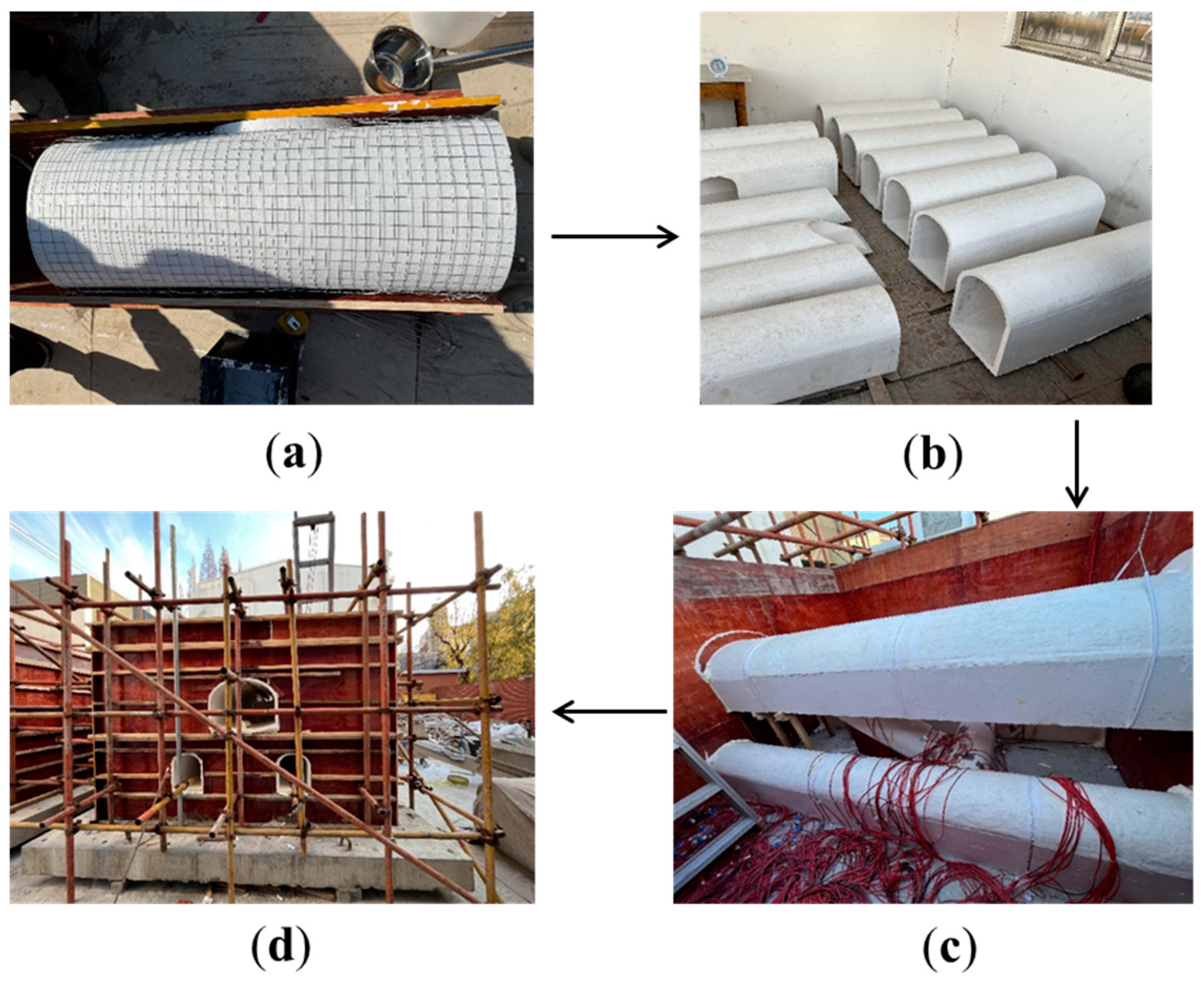
Figure 3.
The complete test models: (a) the homogeneous rock–station model; (b) the jointed rock–station model.
Figure 3.
The complete test models: (a) the homogeneous rock–station model; (b) the jointed rock–station model.
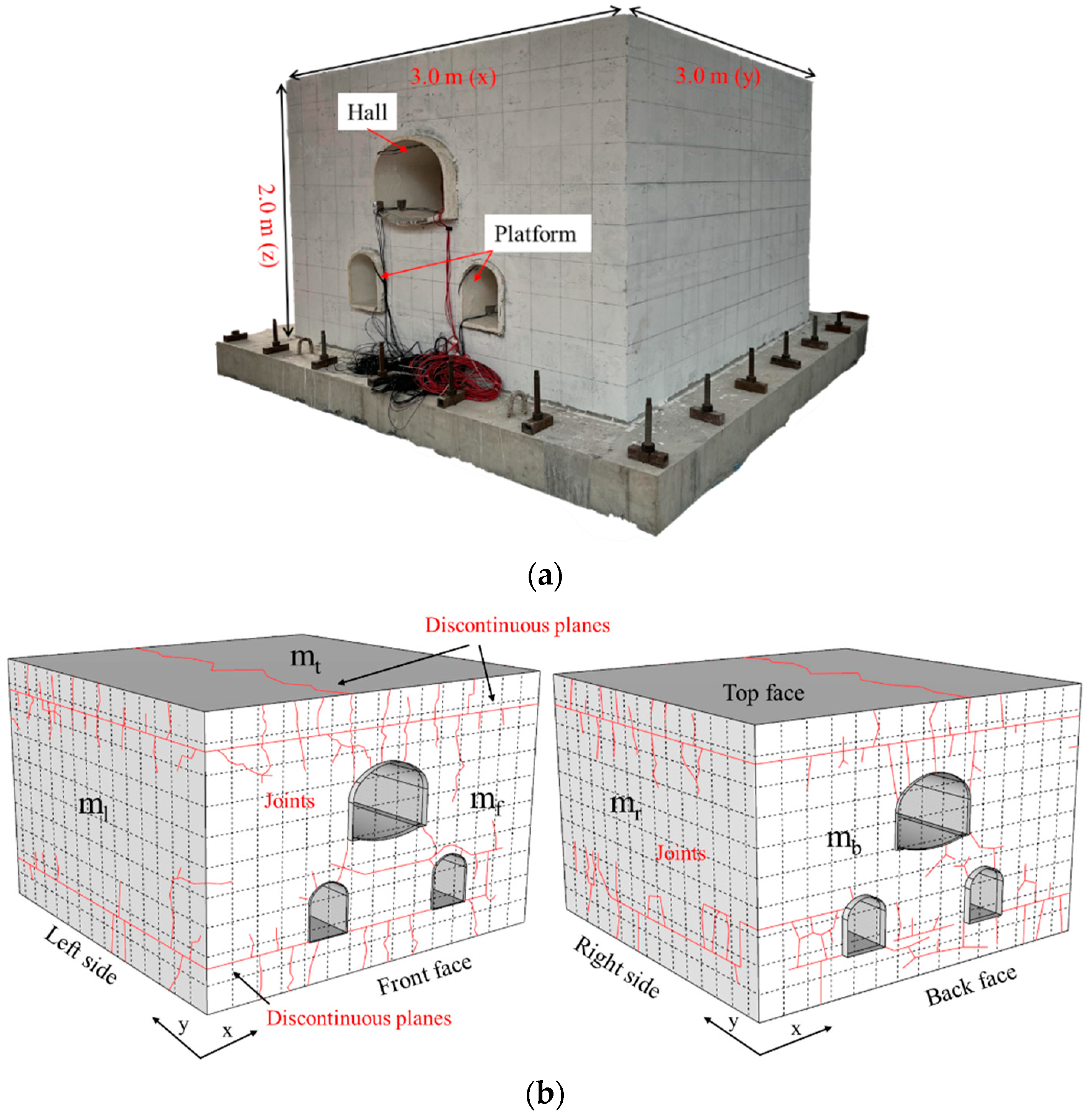
Figure 4.
Layout of sensors: (a) rock accelerometers; (b) structural accelerometers; (c) strain gauges (unit: mm).
Figure 4.
Layout of sensors: (a) rock accelerometers; (b) structural accelerometers; (c) strain gauges (unit: mm).

Figure 5.
Harmonic waveforms.
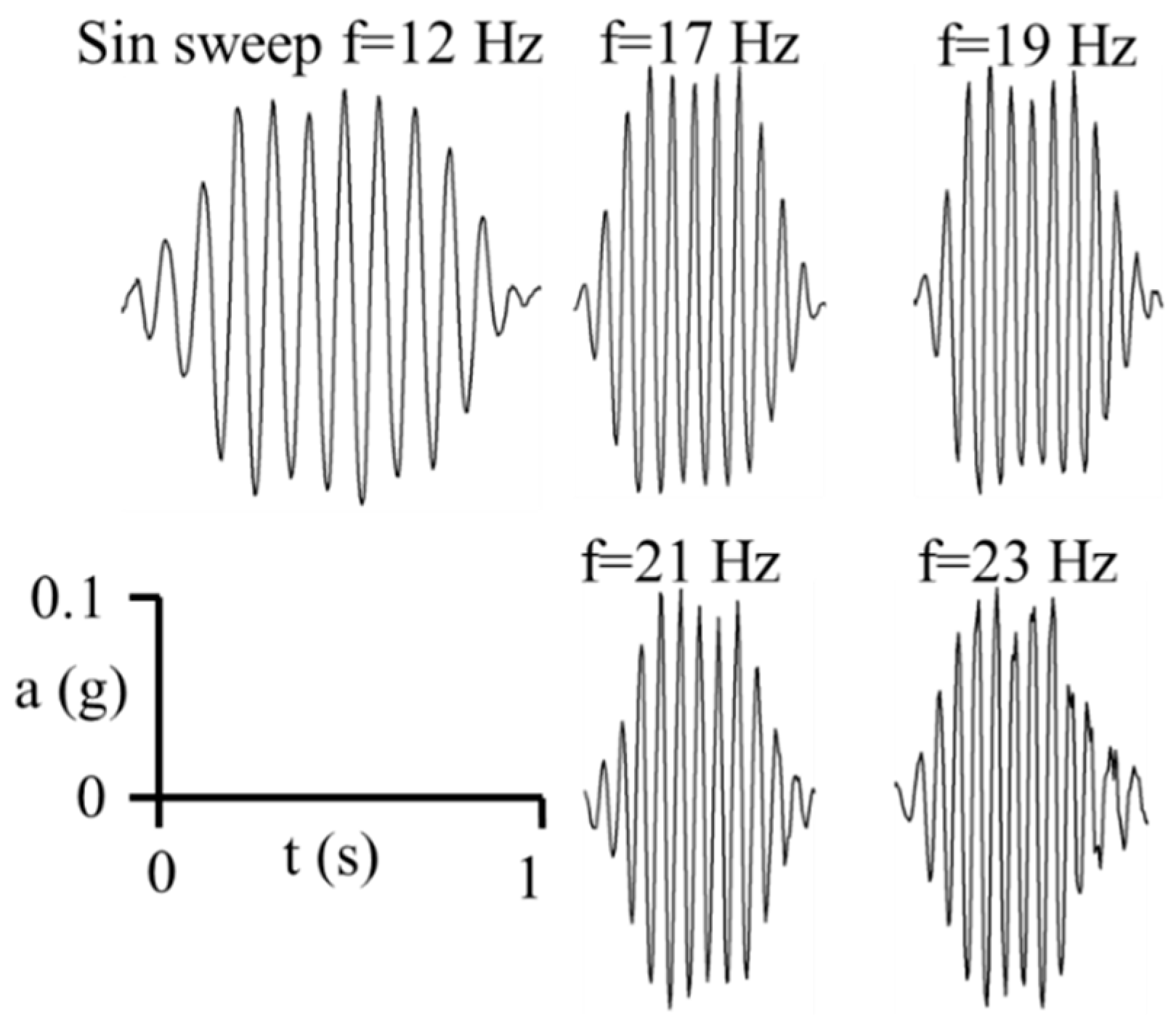
Figure 6.
The acceleration time histories of rock at AS1 and AS2: (a) transverse excitation; (b) longitudinal excitation.
Figure 6.
The acceleration time histories of rock at AS1 and AS2: (a) transverse excitation; (b) longitudinal excitation.
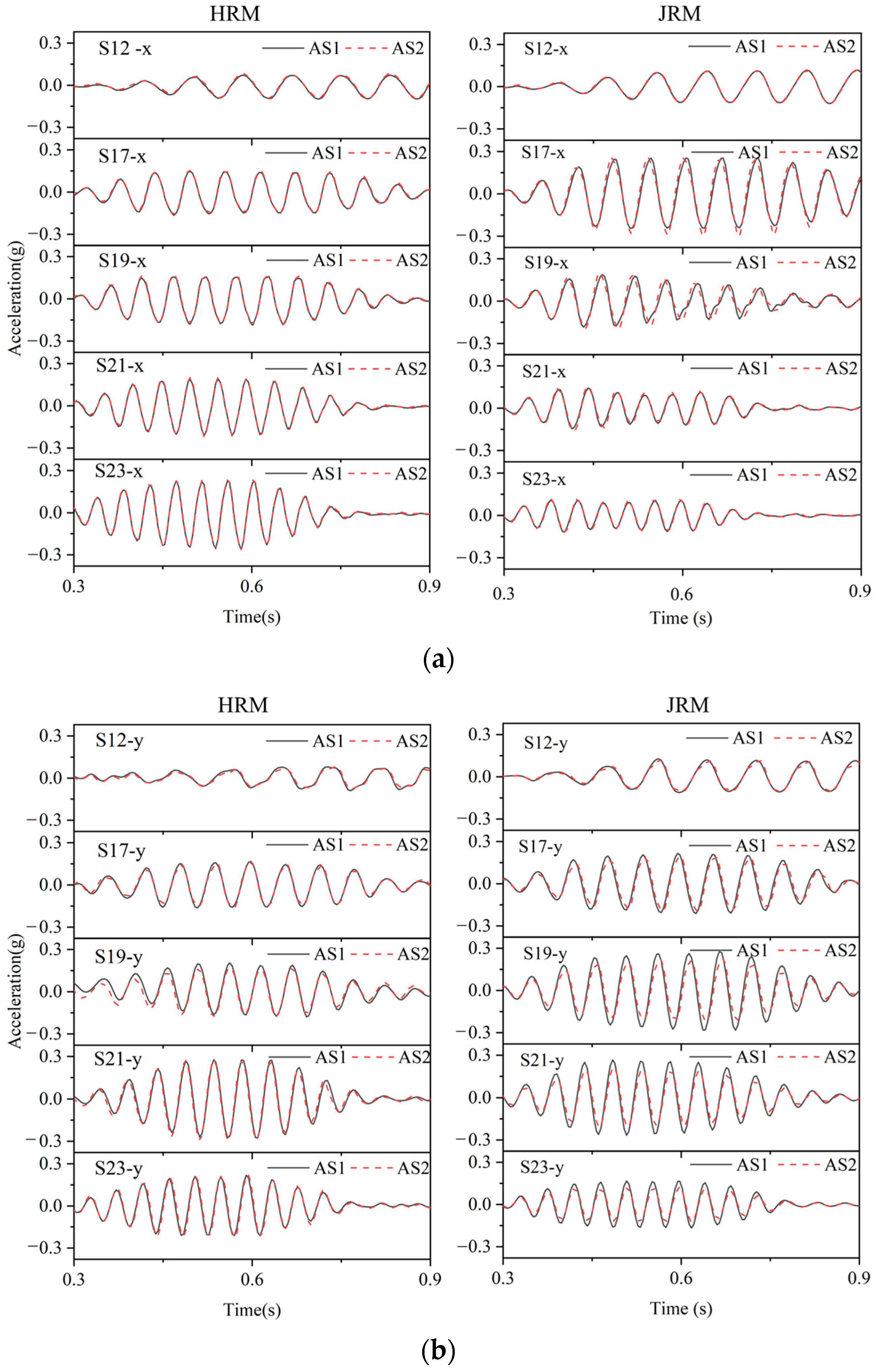
Figure 7.
The acceleration amplification factor (AAF) along the rock height: (a) transverse excitation; (b) longitudinal excitation.
Figure 7.
The acceleration amplification factor (AAF) along the rock height: (a) transverse excitation; (b) longitudinal excitation.
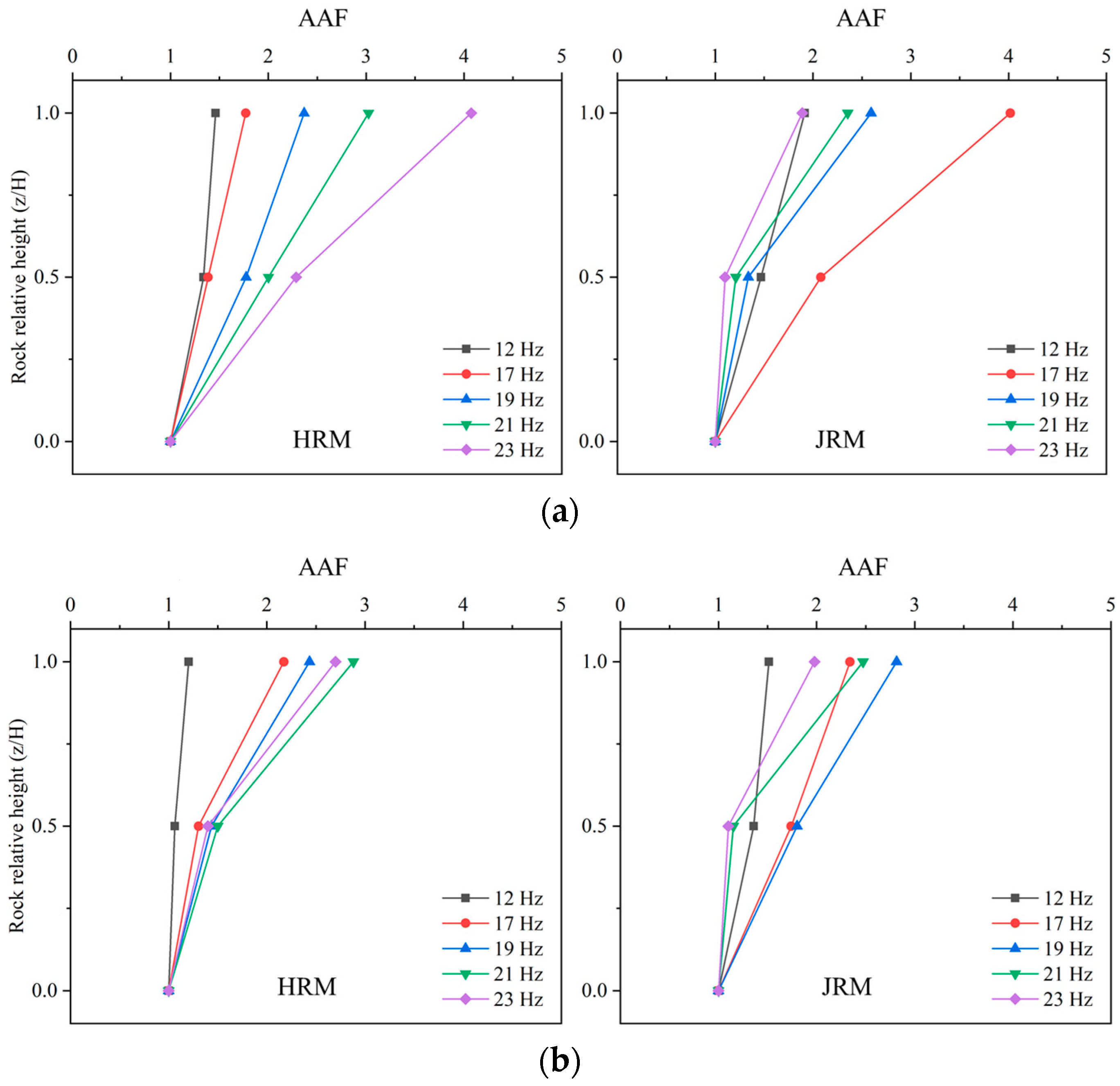
Figure 8.
Comparison of transfer functions for the two models: (a) transverse excitation; (b) longitudinal excitation.
Figure 8.
Comparison of transfer functions for the two models: (a) transverse excitation; (b) longitudinal excitation.

Figure 9.
Acceleration power spectral density of AS0, AS1, and AS2: (a) transverse excitation; (b) longitudinal excitation.
Figure 9.
Acceleration power spectral density of AS0, AS1, and AS2: (a) transverse excitation; (b) longitudinal excitation.

Figure 10.
Comparison of acceleration power spectral density ratio: (a) transverse excitation; (b) longitudinal excitation.
Figure 10.
Comparison of acceleration power spectral density ratio: (a) transverse excitation; (b) longitudinal excitation.
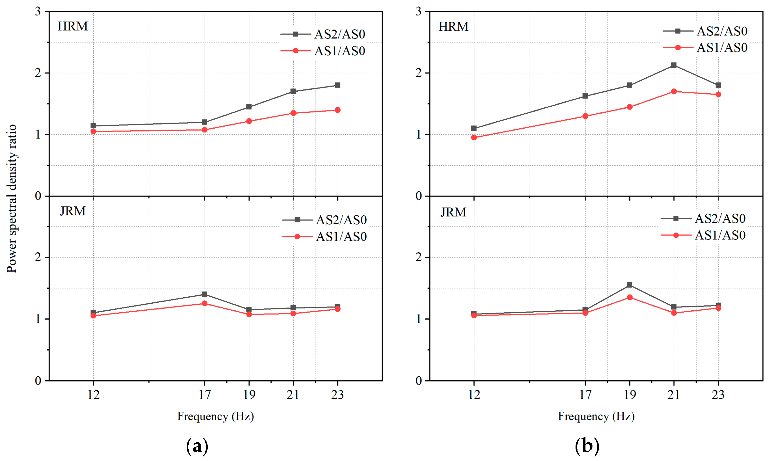
Figure 11.
Acceleration time histories of the main structures: (a) Sine 12 Hz-x; (b) Sine 21 Hz-x; (c) Sine 12 Hz-y; (d) Sine 21 Hz-y.
Figure 11.
Acceleration time histories of the main structures: (a) Sine 12 Hz-x; (b) Sine 21 Hz-x; (c) Sine 12 Hz-y; (d) Sine 21 Hz-y.
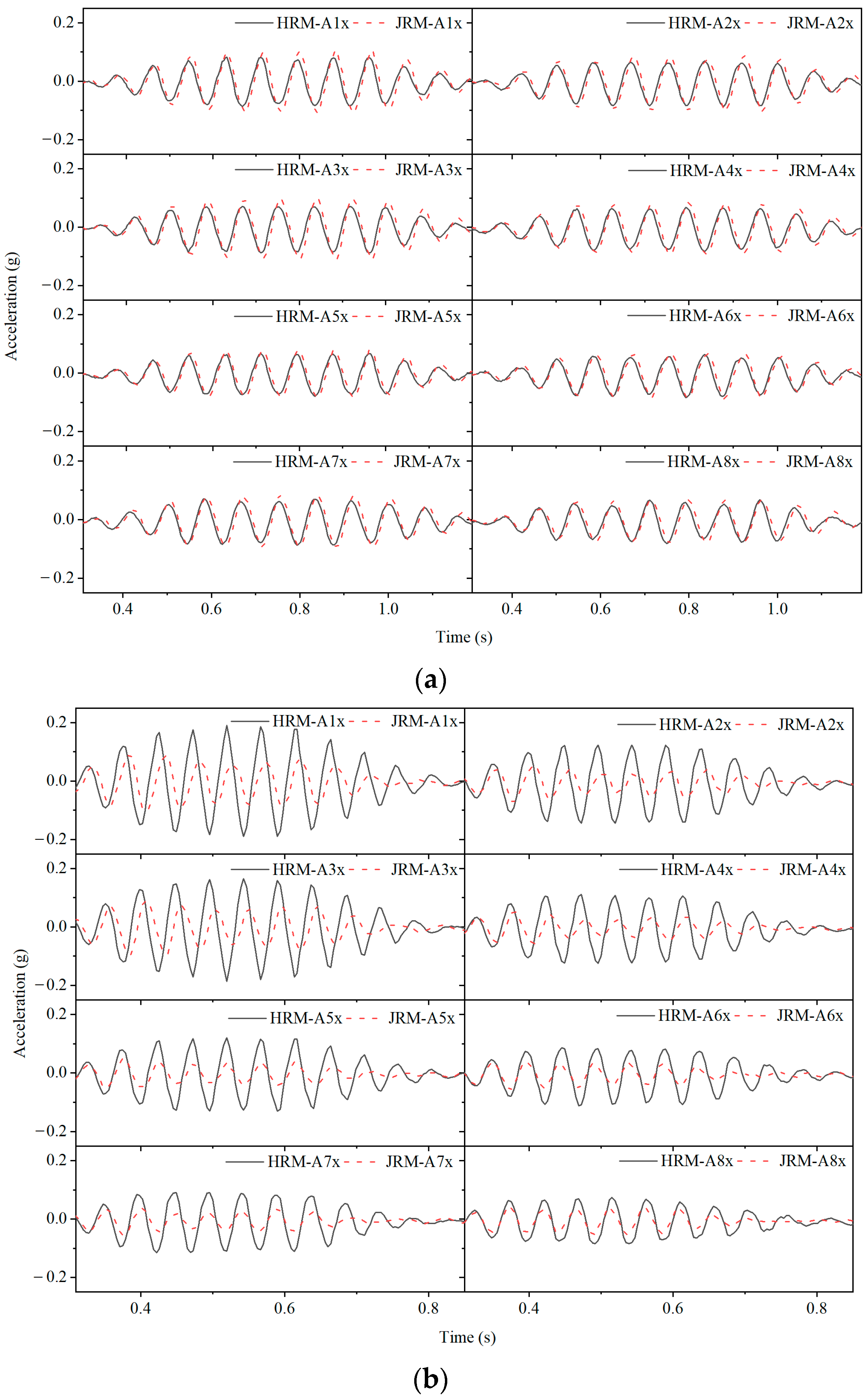
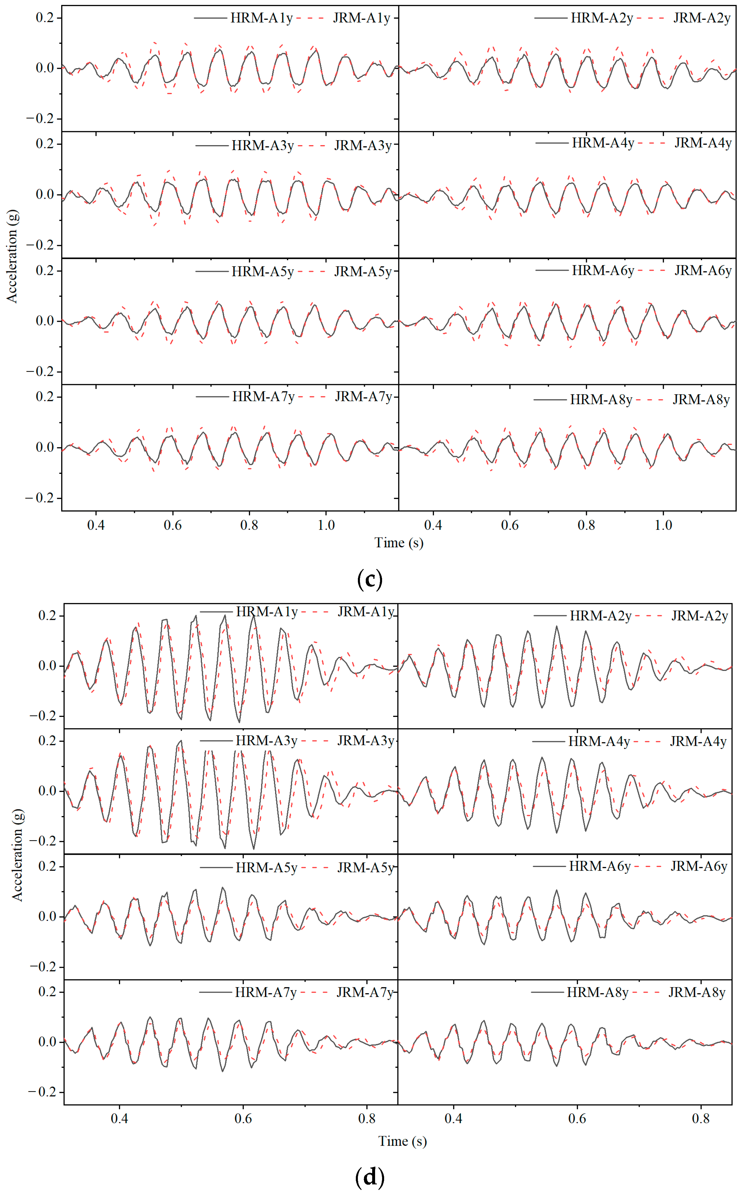
Figure 12.
Acceleration response–frequency curves of the main structures: (a) transverse excitation; (b) longitudinal excitation.
Figure 12.
Acceleration response–frequency curves of the main structures: (a) transverse excitation; (b) longitudinal excitation.
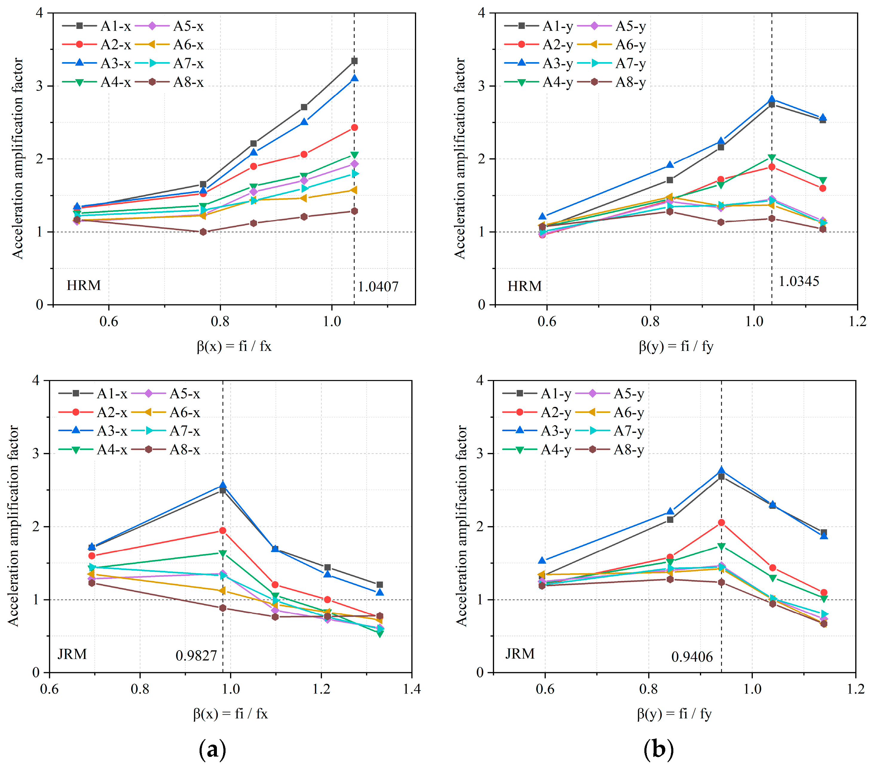
Figure 13.
Energy response–frequency curves of the main structures: (a) transverse excitation; (b) longitudinal excitation.
Figure 13.
Energy response–frequency curves of the main structures: (a) transverse excitation; (b) longitudinal excitation.

Figure 14.
Dynamic strain time histories at structural connections: (a) Sine 17 Hz-x; (b) Sine 17 Hz-y; (c) Sine 19 Hz-x; (d) Sine 19 Hz-y.
Figure 14.
Dynamic strain time histories at structural connections: (a) Sine 17 Hz-x; (b) Sine 17 Hz-y; (c) Sine 19 Hz-x; (d) Sine 19 Hz-y.
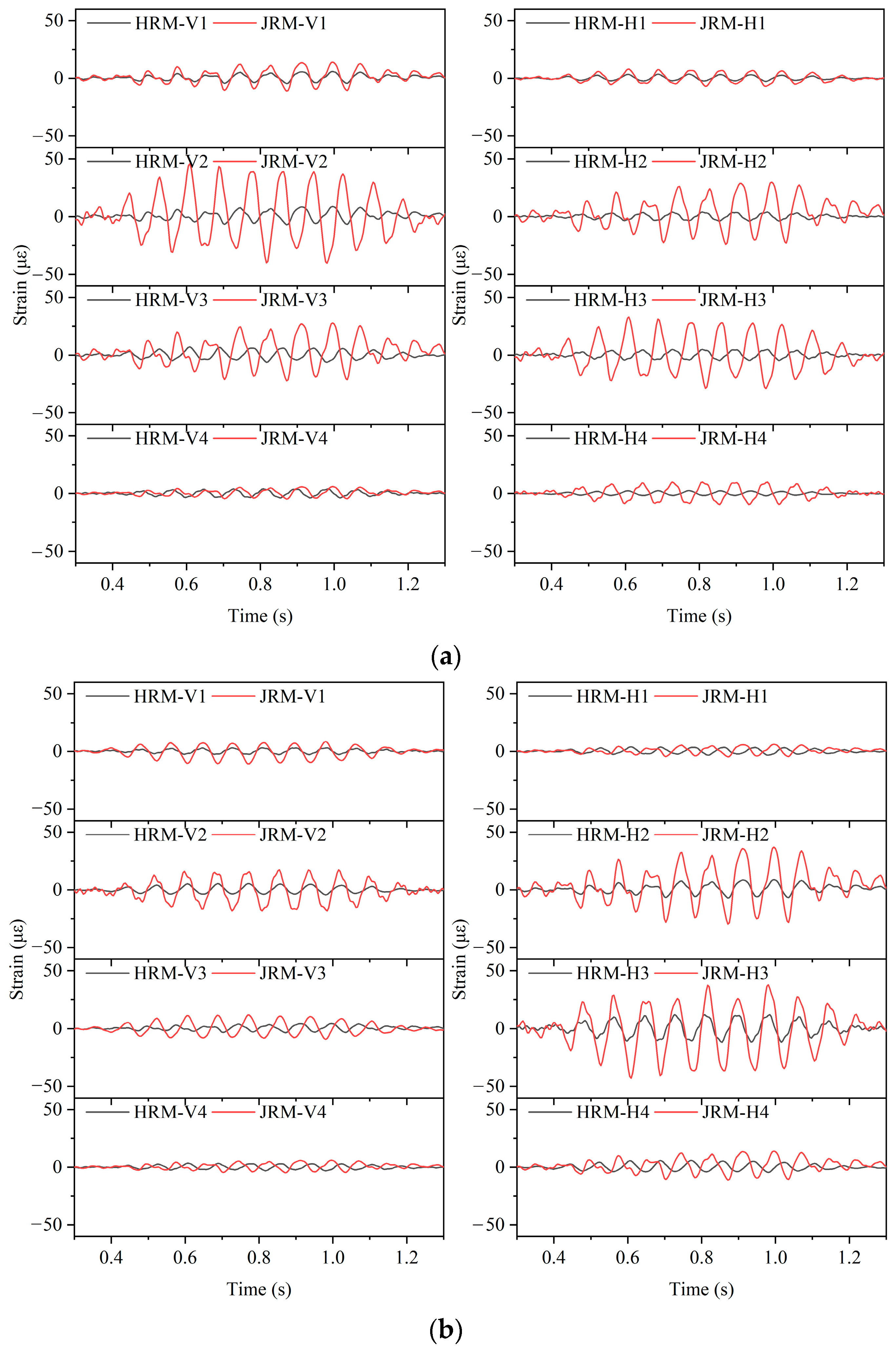
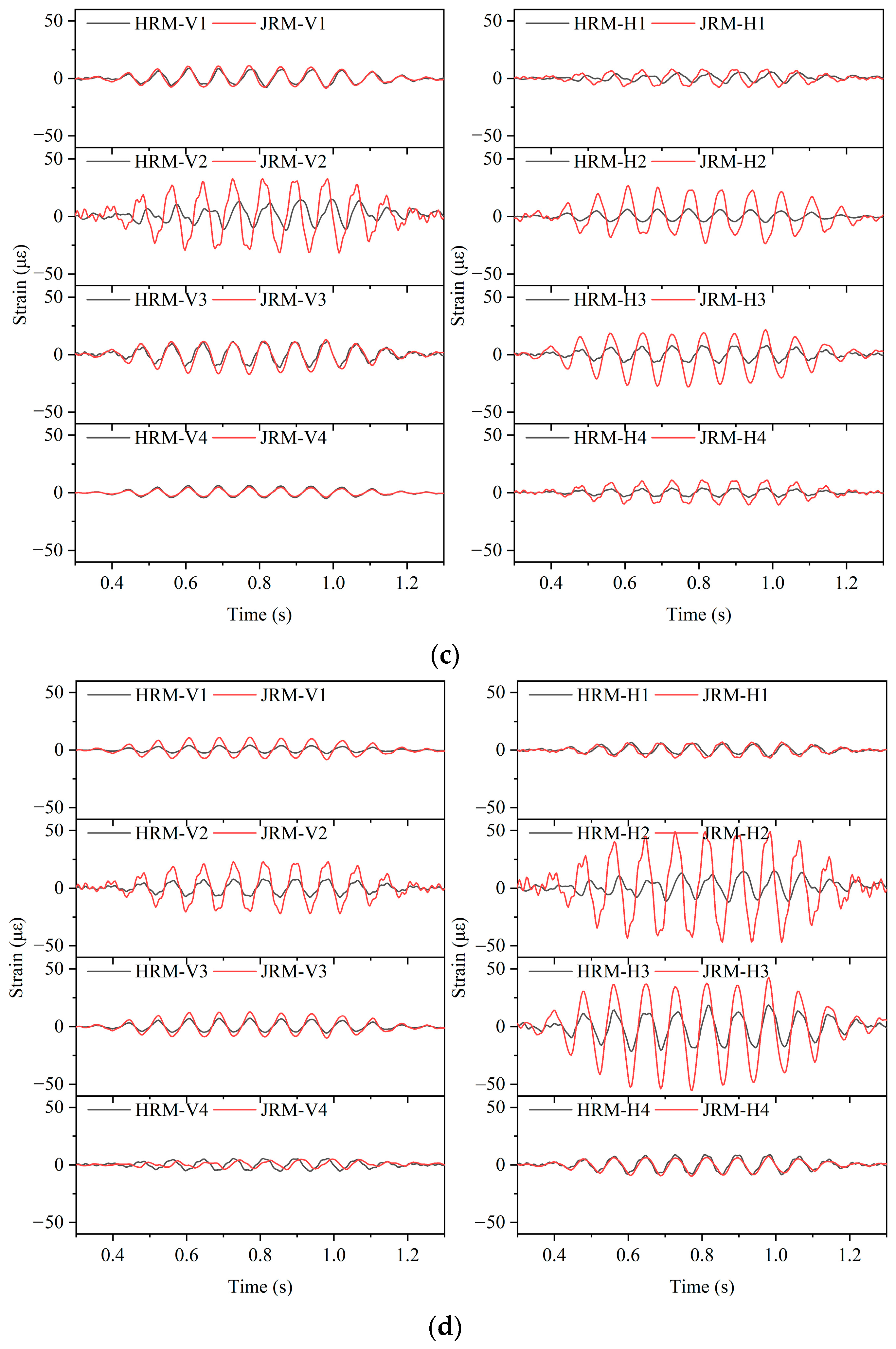
Figure 15.
Peak tensile strains at structural connections: (a) transverse excitation; (b) longitudinal excitation.
Figure 15.
Peak tensile strains at structural connections: (a) transverse excitation; (b) longitudinal excitation.
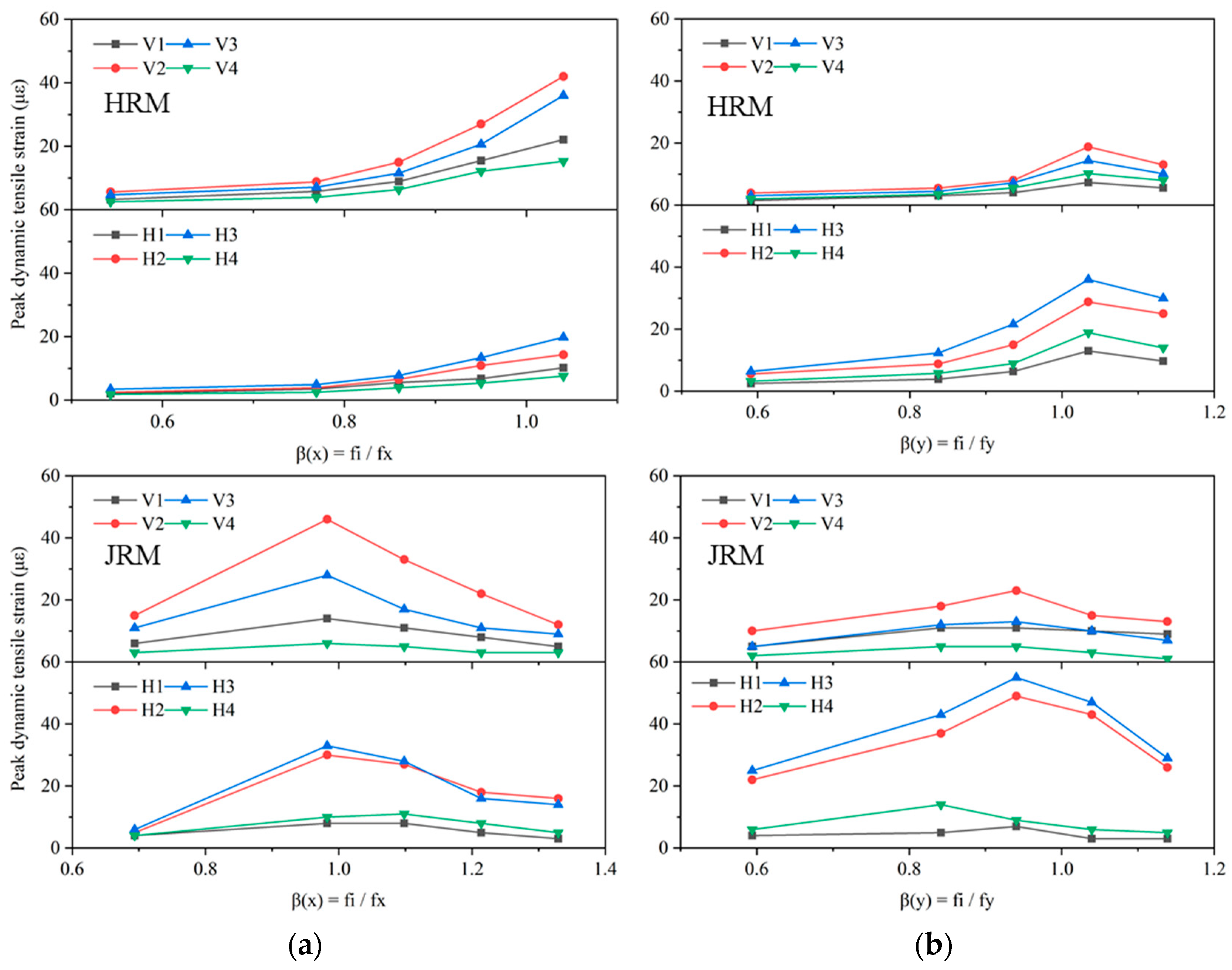
Figure 16.
Peak strain frequency response curves of different measurement points at the same height of the platform: (a) transverse excitation; (b) longitudinal excitation.
Figure 16.
Peak strain frequency response curves of different measurement points at the same height of the platform: (a) transverse excitation; (b) longitudinal excitation.

Table 1.
Similitude relations for the model.
| Item | Expression | Similitude Ratio |
|---|---|---|
| Geometrical | L | 1/30 |
| Density | FT2L−4 | 1/3.33 |
| Young’s modulus | FL−2 | 1/100 |
| Velocity | LT−1 | 1/5.47 |
| Acceleration | LT−2 | 1 |
| Time | T | 1/5.48 |
| Frequency | T−1 | 5.48/1 |
| Strain | / | 1 |
| Stress | FL−2 | 1/100 |
Table 2.
Properties of prototype and model materials.
| Item | Density (Kg/m3) | Elastic Modulus (Mpa) | Poisson’s Ratio | Cohesion (kPa) | Friction Angle (°) | |
|---|---|---|---|---|---|---|
| Rock | Prototype | 2550 | 11000 | 0.3 | 1100 | 27 |
| Target | 765 | 110 | 0.3 | 11 | 27 | |
| Test | 730 | 110 | 0.3 | 15 | 33 | |
| Lining | Prototype | 2500 | 33500 | 0.2 | / | / |
| Target | 750 | 335 | 0.2 | / | / | |
| Test | 720 | 350 | 0.2 | / | / |
Table 3.
Parameters of the joints.
| Joint Sets | Loading Direction | (°) | λ (m−1) | (m) |
|---|---|---|---|---|
| Sides | x | 90 | 0.67 | 1.27 |
| y | 90 | 0.67 | 1.27 | |
| Faces | x | 15 | 0.64 | 2.42 |
| y | 75 | 0.12 | 3.33 |
Table 4.
Test cases for the shaking table tests.
| Test Case | Input Motions | Peak Acceleration (g) | Input Direction |
|---|---|---|---|
| WN1 | white noise | 0.05 | xy |
| S12-x | Sine-12 Hz | 0.1 | x |
| S17-x | Sine-17 Hz | ||
| S19-x | Sine-19 Hz | ||
| S21-x | Sine-21 Hz | ||
| S23-x | Sine-23 Hz | ||
| S12-y | Sine-12 Hz | 0.1 | y |
| S17-y | Sine-17 Hz | ||
| S19-y | Sine-19 Hz | ||
| S21-y | Sine-21 Hz | ||
| S23-y | Sine-23 Hz |
Table 5.
Difference in acceleration amplification factors of the measurement points.
| Model | FRF | Hall | Platform | ||||||
|---|---|---|---|---|---|---|---|---|---|
| A1/A2 | A3/A4 | A1/A3 | A2/A4 | A5/A6 | A7/A8 | A5/A7 | A6/A8 | ||
| HRM | 1.38 | 1.45 | 1.11 | 1.18 | 1.23 | 1.40 | 1.07 | 1.22 | |
| 1.45 | 1.39 | 0.98 | 0.93 | 1.06 | 1.21 | 1.01 | 1.15 | ||
| JRM | 1.28 | 1.56 | 0.97 | 1.19 | 1.20 | 1.50 | 1.02 | 1.27 | |
| 1.31 | 1.59 | 0.97 | 1.18 | 1.03 | 1.17 | 1.01 | 1.15 | ||
Disclaimer/Publisher’s Note: The statements, opinions and data contained in all publications are solely those of the individual author(s) and contributor(s) and not of MDPI and/or the editor(s). MDPI and/or the editor(s) disclaim responsibility for any injury to people or property resulting from any ideas, methods, instructions or products referred to in the content. |
© 2024 by the authors. Licensee MDPI, Basel, Switzerland. This article is an open access article distributed under the terms and conditions of the Creative Commons Attribution (CC BY) license (https://creativecommons.org/licenses/by/4.0/).
Share and Cite
MDPI and ACS Style
Li, R.; Yuan, Y. Effect of Jointed Rock Mass on Seismic Response of Metro Station Tunnel-Group Structures. Appl. Sci. 2024, 14, 4080. https://doi.org/10.3390/app14104080
AMA Style
Li R, Yuan Y. Effect of Jointed Rock Mass on Seismic Response of Metro Station Tunnel-Group Structures. Applied Sciences. 2024; 14(10):4080. https://doi.org/10.3390/app14104080
Chicago/Turabian StyleLi, Ruozhou, and Yong Yuan. 2024. "Effect of Jointed Rock Mass on Seismic Response of Metro Station Tunnel-Group Structures" Applied Sciences 14, no. 10: 4080. https://doi.org/10.3390/app14104080
Note that from the first issue of 2016, this journal uses article numbers instead of page numbers. See further details here.