

The Estimation of Shear Wave Velocity for Shallow Underground Structures in the Central Himalaya Region of Nepal

 ,
,
Abstract
:1. Background
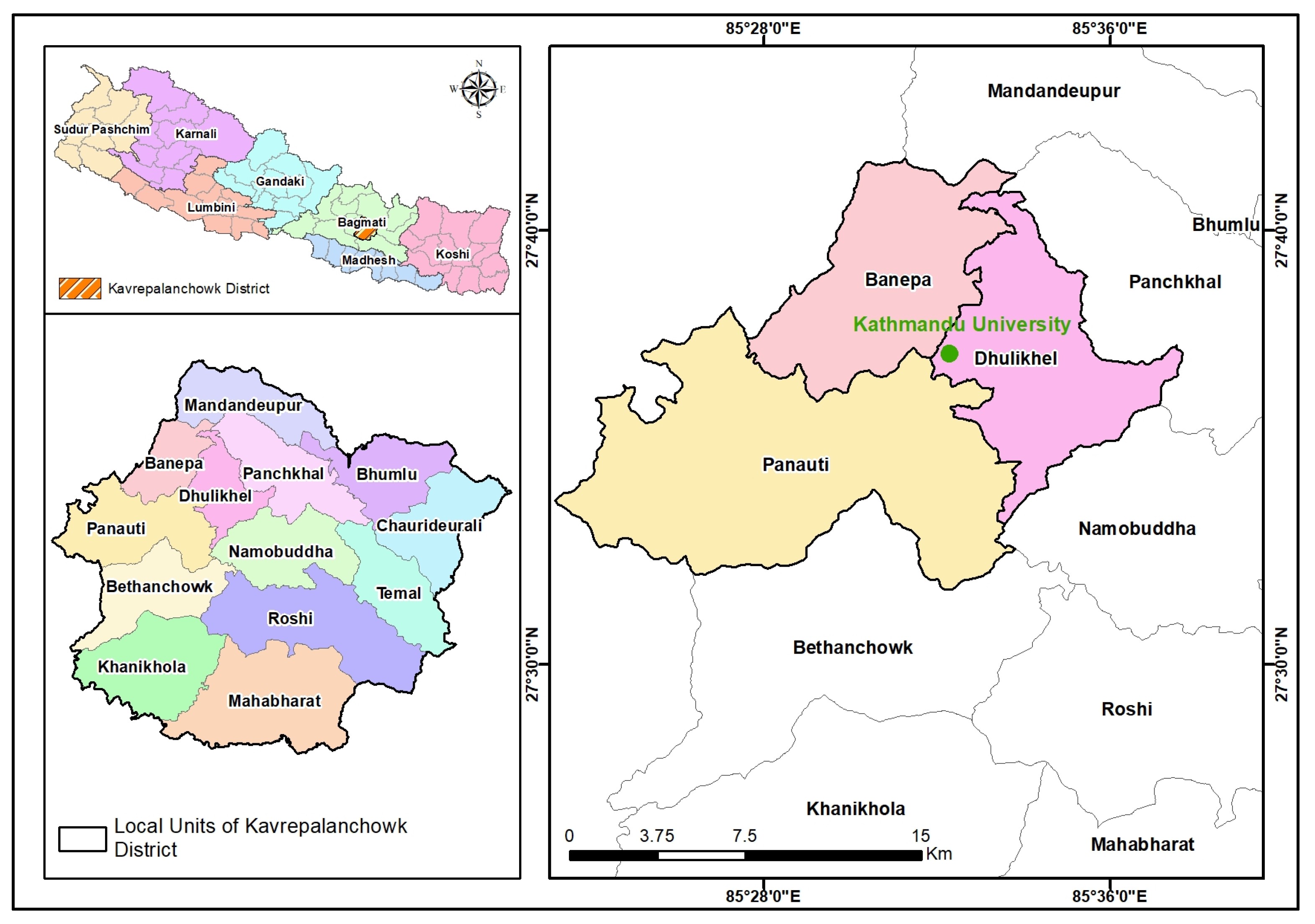
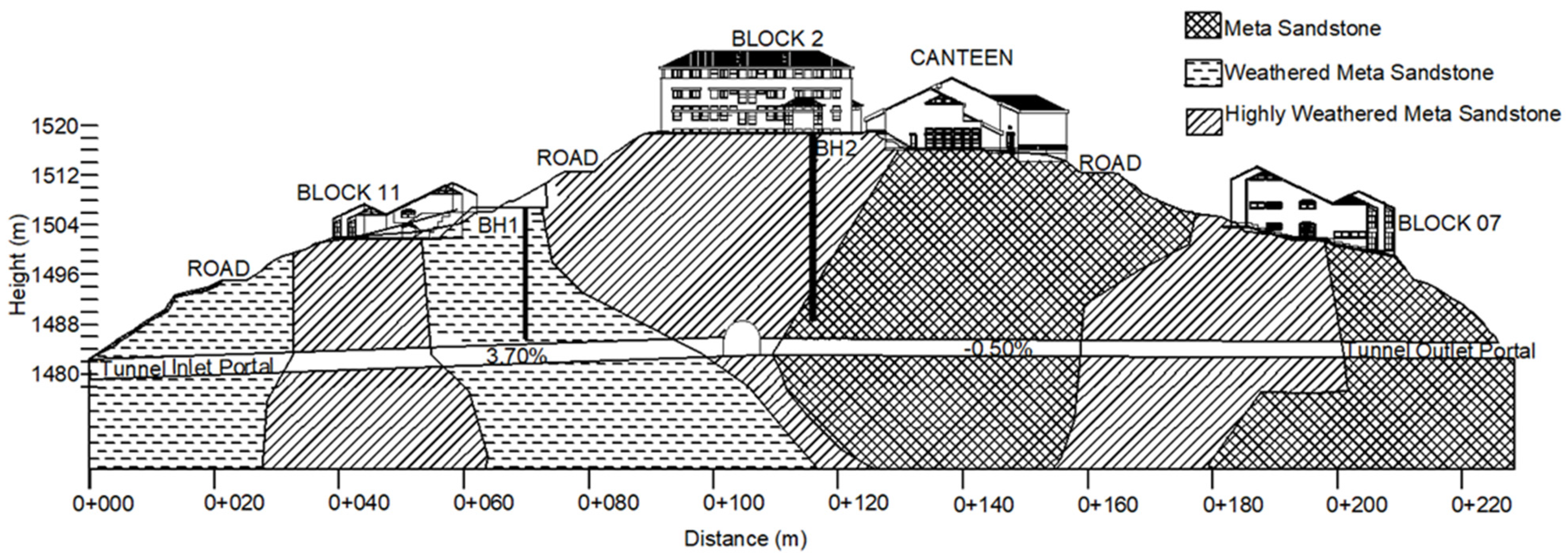
2. Study Area
3. Insight into Calculation of Shear Wave Velocities
3.1. Geotechnical Investigation
3.2. Geophysical Investigation
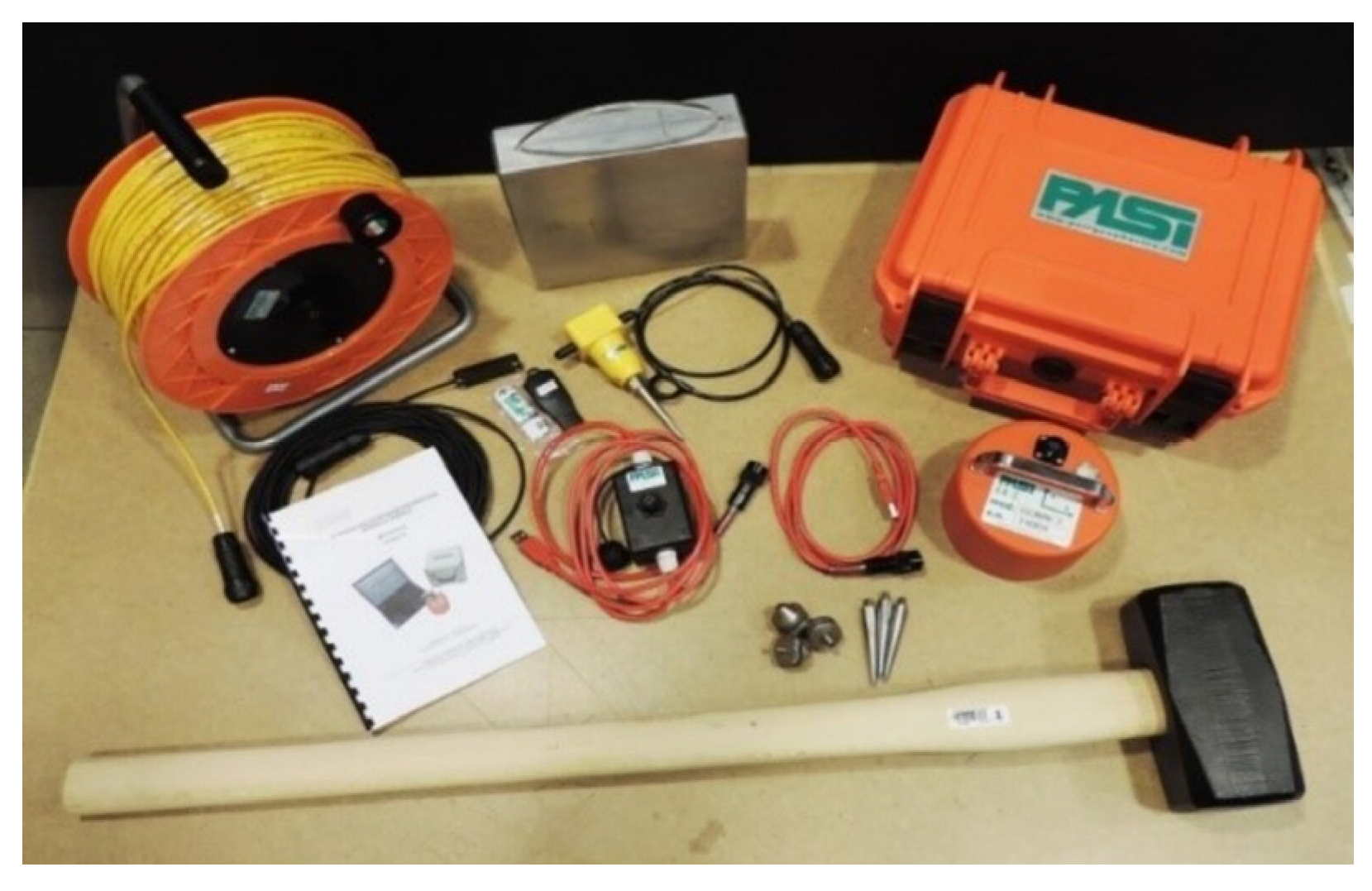
3.2.1. Multichannel Analysis of Surface Waves (MASW)
3.2.2. Microtremor Array Measurement (MAM)
3.3. Soil Profile
4. Results
4.1. Geotechnical Investigation
4.2. Geophysical Investigation
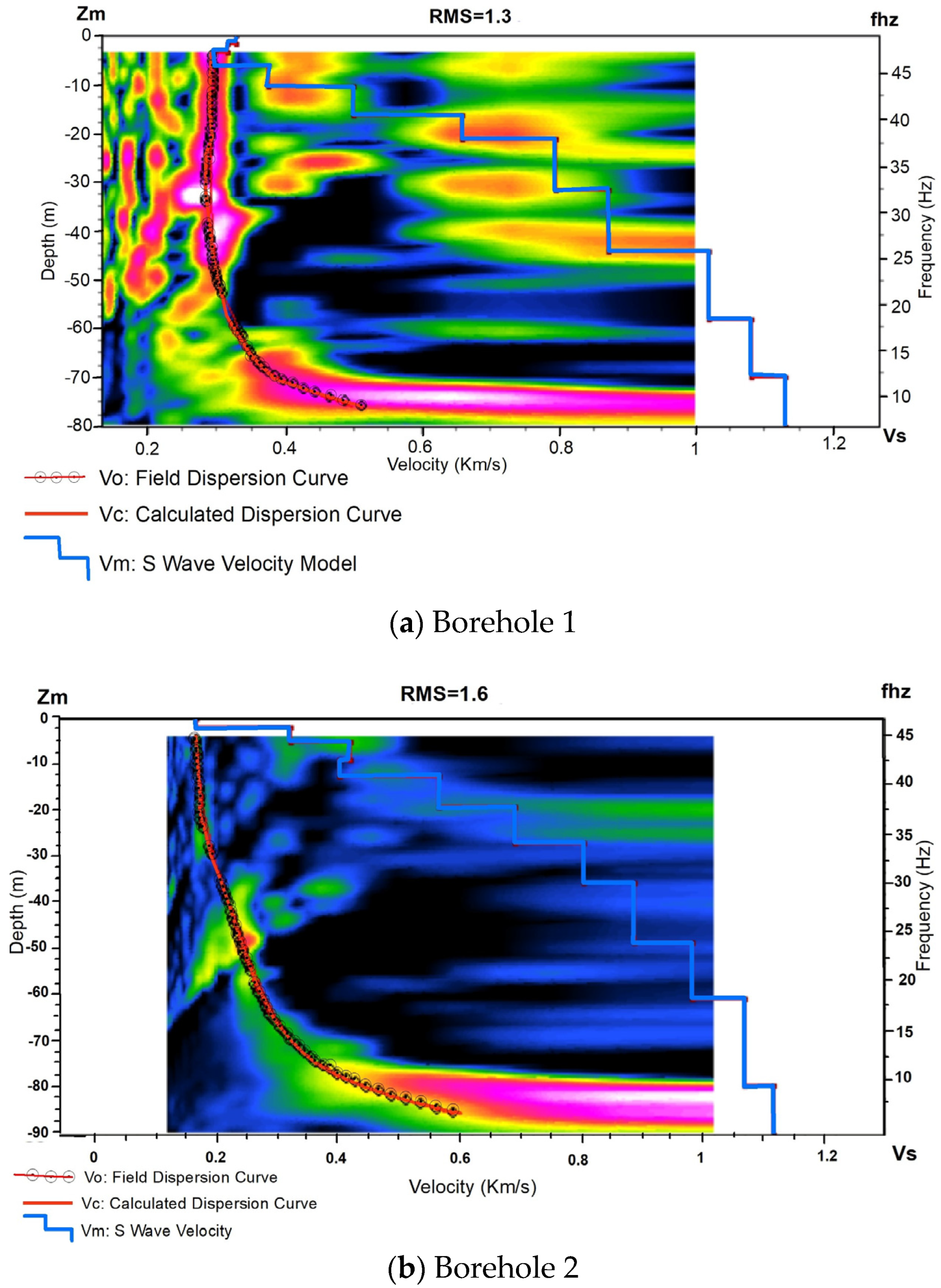
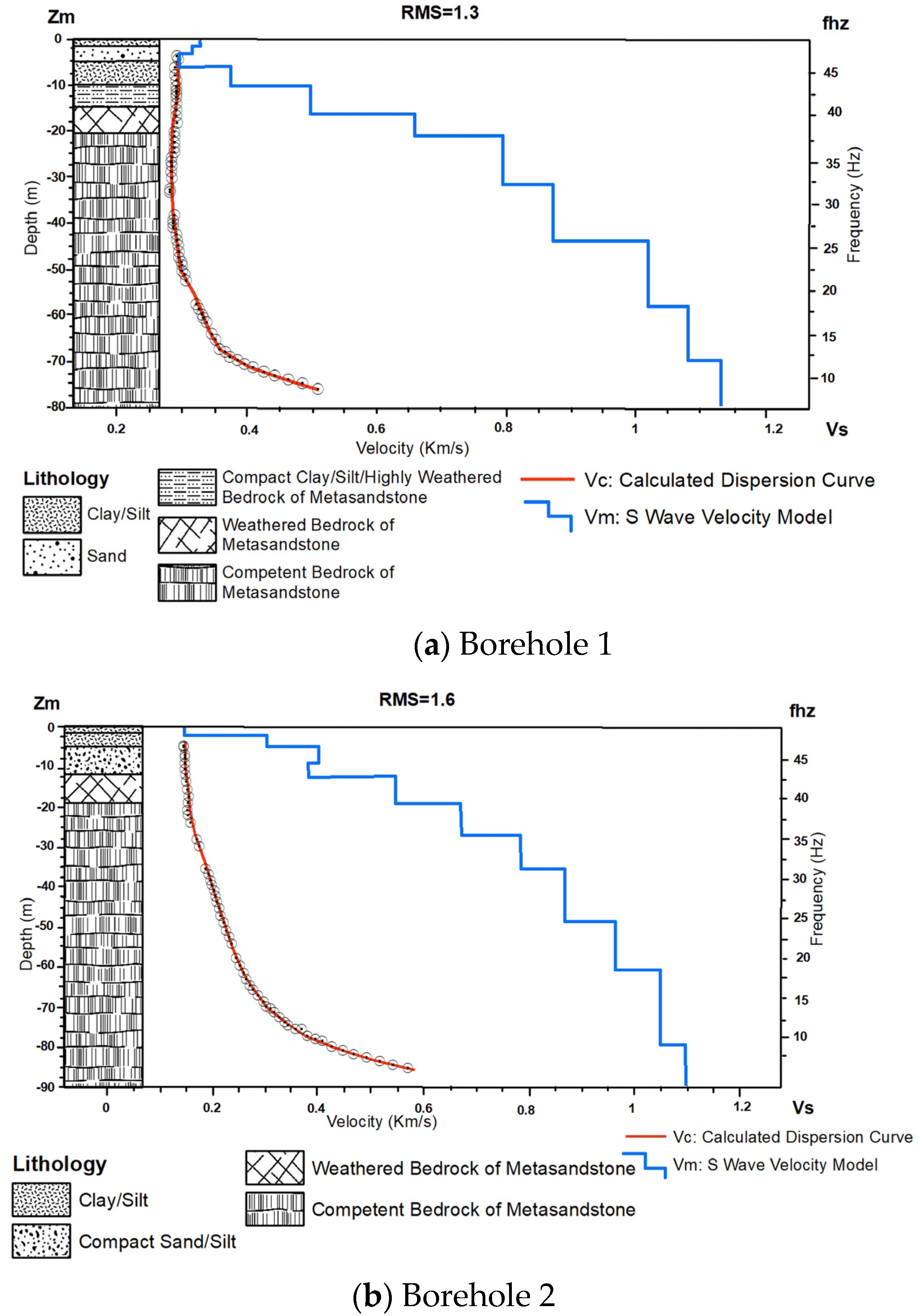
4.2.1. MASW
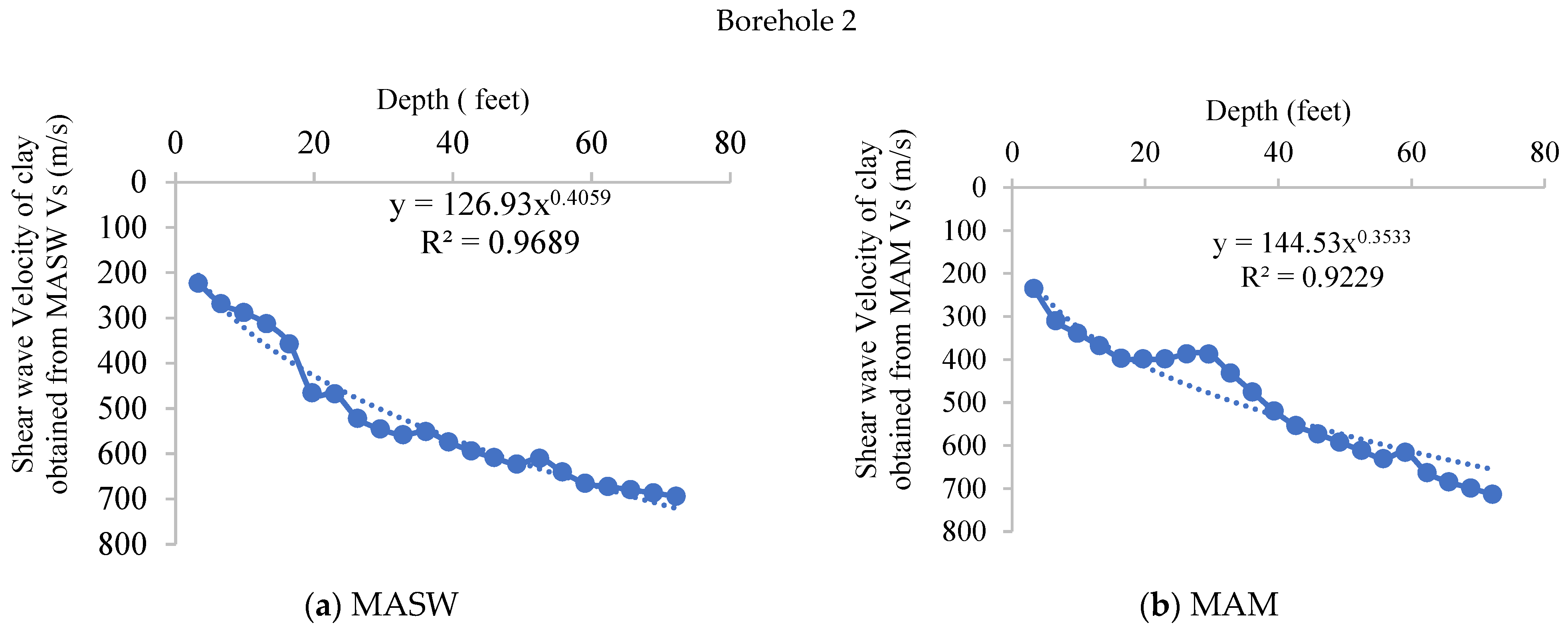
4.2.2. MAM
5. Conclusions
Author Contributions
Funding
Data Availability Statement
Acknowledgments
Conflicts of Interest
References
- Ambraseys, N.N.; Douglas, J. Magnitude Calibration of North Indian Earthquakes. Geophys. J. Int. 2004, 159, 165–206. [Google Scholar] [CrossRef]
- BECA. Seismic Hazard Mapping and Risk Assessment for Nepal; UNDP/HMGN/UNCHS (Habitat) Subproject NEP/88/054/21.03; BECA World International: Auckland, New Zealand, 1993. [Google Scholar]
- Parajuli, H.R.; Bhusal, B.; Paudel, S. Seismic Zonation of Nepal Using Probabilistic Seismic Hazard Analysis. Arab. J. Geosci. 2021, 14, 1–14. [Google Scholar] [CrossRef]
- Khadka, S.S. Tunnel Closure Analysis of Hydropower Tunnels in Lesser Himalayan Region of Nepal through Case Studies. Ph.D. Thesis, Kathmandu Univeristy, Dhulikhel, Nepal, 2019. [Google Scholar]
- NBC. 105 Seismic Design of Buildings in Nepal; NBC: New York, NY, USA, 2020. [Google Scholar]
- Parajuli, H.R. Seismic Hazard Assessment of Kavre Valley Municipalities. In Proceedings of the IOE Graduate Conference; Tribhuvan University: Kathmandu, Nepal, 2015; pp. 193–201. [Google Scholar]
- Yoshida, M. Neogene to Quaternary Lacustrine Sediments in the Kathmandu Valley, Nepal. J. Nepal Geol. Soc. 1984, 4, 73–100. [Google Scholar]
- Dill, H.G.; Khadka, D.R.; Khanal, R.; Dohrmann, R.; Melcher, F.; Busch, K. Infilling of the Younger Kathmandu–Banepa Intermontane Lake Basin during the Late Quaternary (Lesser Himalaya, Nepal): A Sedimentological Study. J. Quat. Sci. Publ. Quat. Res. Assoc. 2003, 18, 41–60. [Google Scholar] [CrossRef]
- Stöcklin, J.; Bhattarai, K.D. Geology of Kathmandu Area and Central Mahabharat Range; Nepal Himalaya HMG/UNDP Mineral Exploration Project; Technical Report; UNDP: Kathamandu, Nepal, 1981. [Google Scholar]
- Gaha, T.B.; Bhusal, B.; Paudel, S.; Saru, S. Investigation of Ground Response Analysis for Kathmandu Valley: A Case Study of Gorkha Earthquake. Arab. J. Geosci. 2022, 15, 1354. [Google Scholar] [CrossRef]
- Chetri, M. Geomorphological Evolution of Banepa Valley. M.Sc. Dissertation, Central Department of Geology, Tribhuvan University, Kathmandu, Nepal, 1993, Volume 60, unpublished. [Google Scholar]
- Dongol, G. Geology of the Kathmandu Fluvial Lacustrine Sediments in the Light of New Vertebrate Fossil Occurrences. J. Nepal Geol. Soc. 1985, 3, 43–57. [Google Scholar]
- Sakai, H.; Fujii, R.; Kuwahara, Y. Changes in the Depositional System of the Paleo-Kathmandu Lake Caused by Uplift of the Nepal Lesser Himalayas. J. Asian Earth Sci. 2002, 20, 267–276. [Google Scholar] [CrossRef]
- Moribayashi, S.; Maruo, Y. Basement Topography of the Kathmandu Valley, Nepal An Application of Gravitational Method to the Survey of a Tectonic Basin in the Himalayas. J. Jpn. Soc. Eng. Geol. 1980, 21, 80–87. [Google Scholar] [CrossRef]
- Igarashi, Y.; Yoshida, M. History of vegetation and climate in the kathmandu valley. Proc. Indian Natn. Sci. Acad. 1988, 54, 550–563. [Google Scholar]
- Dahal, R.K.; Aryal, A. Geotechnical Properties of Soil at Sundhara and Jamal Area in Kathmandu, Nepal. J. Nepal Geol. Soc. 2002, 27, 77–86. [Google Scholar] [CrossRef]
- Kumahara, Y.; Chamlagain, D.; Upreti, B.N. Geomorphic Features of Active Faults around the Kathmandu Valley, Nepal, and No Evidence of Surface Rupture Associated with the 2015 Gorkha Earthquake along the Faults. Earth Planets Space 2016, 68, 1–8. [Google Scholar] [CrossRef]
- Verma, M.; Singh, R.; Bansal, B. Soft Sediments and Damage Pattern: A Few Case Studies from Large Indian Earthquakes Vis-a-Vis Seismic Risk Evaluation. Nat. Hazards 2014, 74, 1829–1851. [Google Scholar] [CrossRef]
- Bard, P.-Y.; Riepl-Thomas, J. Wave Propagation in Complex Geological Structures and Their Effects on Strong Ground Motion. In Wave Motion in Earthquake Engineering; Kausel, E., Manolis, G., Eds.; WIT Press: Sothampton, UK; Boston, MA, USA, 2000; pp. 37–95. [Google Scholar]
- Kramer, S.L. Geotechnical Earthquake Engineering; Pearson Education: Noida, India, 1996; ISBN 81-317-0718-0. [Google Scholar]
- Bhusal, B.; Aaqib, M.; Paudel, S.; Parajuli, H.R. Site Specific Seismic Hazard Analysis of Monumental Site Dharahara, Kathmandu, Nepal. Geomat. Nat. Hazards Risk 2022, 13, 2674–2696. [Google Scholar] [CrossRef]
- Thapa, U.J.; Karki, S.; Khadka, S.S. Seismic Assessment of Underground Structures in the Weak Himalayan Rock Mass for Hydropower Development; IOP Publishing: Bristol, UK, 2023; Volume 2629, p. 012014. [Google Scholar] [CrossRef]
- Celebi, M.; Prince, J.; Dietel, C.; Onate, M.; Chavez, G. The Culprit in Mexico City—Amplification of Motions. Earthq. Spectra 1987, 3, 315–328. [Google Scholar] [CrossRef]
- Seed, R.B. Preliminary Report on the Principal Geotechnical Aspects of the October 17, 1989, Loma Prieta Earthquake; Report No UCBEERC-9005; University of California, Berkeley, Earthquake Engineering Research Center: Berkeley, CA, USA, 1990. [Google Scholar]
- Stewart, J.P. Benchmarking of Nonlinear Geotechnical Ground Response Analysis Procedures; Pacific Earthquake Engineering Research Center: Berkeley, CA, USA, 2008. [Google Scholar]
- Griffiths, S.C.; Cox, B.R.; Rathje, E.M. Challenges Associated with Site Response Analyses for Soft Soils Subjected to High-Intensity Input Ground Motions. Soil Dyn. Earthq. Eng. 2016, 85, 1–10. [Google Scholar] [CrossRef]
- Stewart, J.P.; Kwok, A.O. Nonlinear Seismic Ground Response Analysis: Code Usage Protocols and Verification against Vertical Array Data. In Geotechnical Earthquake Engineering and Soil Dynamics IV; American Society of Civil Engineers: Reston, VA, USA, 2008; pp. 1–24. [Google Scholar]
- Yee, E.; Stewart, J.P.; Tokimatsu, K. Elastic and Large-Strain Nonlinear Seismic Site Response from Analysis of Vertical Array Recordings. J. Geotech. Geoenvironmental Eng. 2013, 139, 1789–1801. [Google Scholar] [CrossRef]
- Kwok, A.O.; Stewart, J.P.; Hashash, Y.M. Nonlinear Ground-Response Analysis of Turkey Flat Shallow Stiff-Soil Site to Strong Ground Motion. Bull. Seismol. Soc. Am. 2008, 98, 331–343. [Google Scholar] [CrossRef]
- Hashash, Y.M.; Phillips, C.; Groholski, D.R. Recent Advances in Non-Linear Site Response Analysis. In Proceedings of the 5th International Conference on Recent Advances in Geotechnical Earthquake Engineering and Soil Dynamics, San Diego, CA, USA, 28 May 2010. [Google Scholar]
- Alexopoulos, J.D.; Voulgaris, N.; Dilalos, S.; Gkosios, V.; Giannopoulos, I.-K.; Mitsika, G.S.; Vassilakis, E.; Sakkas, V.; Kaviris, G. Near-Surface Geophysical Characterization of Lithologies in Corfu and Lefkada Towns (Ionian Islands, Greece). Geosciences 2022, 12, 446. [Google Scholar] [CrossRef]
- Mohammed, M.; Abudeif, A.; Abd El-aal, A. Engineering Geotechnical Evaluation of Soil for Foundation Purposes Using Shallow Seismic Refraction and MASW in 15th Mayo, Egypt. J. Afr. Earth Sci. 2020, 162, 103721. [Google Scholar] [CrossRef]
- Hutchinson, P.J.; Beird, M.H. A Comparison of Surface-and Standard Penetration Test-Derived Shear-Wave Velocity. Environ. Eng. Geosci. 2016, 22, 27–36. [Google Scholar] [CrossRef]
- Bullen, K.E. An Introduction to the Theory of Seismology, 3rd ed.; Cambridge University Press: London, UK, 1963; p. 381. [Google Scholar]
- Kirar, B.; Maheshwari, B.K.; Muley, P. Correlation between Shear Wave Velocity (Vs) and SPT Resistance (N) for Roorkee Region. Int. J. Geosynth. Ground Eng. 2016, 2, 1–11. [Google Scholar] [CrossRef]
- Al-Heety, A.J.; Hassouneh, M.; Abdullah, F.M. Application of MASW and ERT Methods for Geotechnical Site Characterization: A Case Study for Roads Construction and Infrastructure Assessment in Abu Dhabi, UAE. J. Appl. Geophys. 2021, 193, 104408. [Google Scholar] [CrossRef]
- Cardarelli, E.; Cercato, M.; De Donno, G. Characterization of an Earth-Filled Dam through the Combined Use of Electrical Resistivity Tomography, P-and SH-Wave Seismic Tomography and Surface Wave Data. J. Appl. Geophys. 2014, 106, 87–95. [Google Scholar] [CrossRef]
- Rezaei, S.; Choobbasti, A.J. Evaluation of Local Site Effect from Microtremor Measurements in Babol City, Iran. J. Seismol. 2018, 22, 471–486. [Google Scholar] [CrossRef]
- Dobrin, M.B.; Savit, C.H. Introduction to Geophysical Prospecting; McGraw-Hill, Inc.: New York, NY, USA, 1988; p. 867. [Google Scholar]
- Lunne, T. Cone Penetration Testing in Geotechnical Practice; Blackie Academic & Professional; Hall Publisher: London, UK, 1997; p. 312. [Google Scholar]
- Park, C.B.; Miller, R.D.; Xia, J. Multichannel Analysis of Surface Waves. Geophysics 1999, 64, 800–808. [Google Scholar] [CrossRef]
- Horike, M. Inversion of Phase Velocity of Long-Period Microtremors to the S-Wave-Velocity Structure down to the Basement in Urbanized Areas. J. Phys. Earth 1985, 33, 59–96. [Google Scholar] [CrossRef]
- Jones, R. In-Situ Measurement of the Dynamic Properties of Soil by Vibration Methods. Geotechnique 1958, 8, 1–21. [Google Scholar] [CrossRef]
- Asten, M.W.; Henstridge, J.D. Array Estimators and the Use of Microseisms for Reconnaissance of Sedimentary Basins. Geophysics 1984, 49, 1828–1837. [Google Scholar] [CrossRef]
- Miller, R.D.; Xia., J.; Ivanov, J. Multichannel Analysis of Surface Waves to Map Bedrock. In The Leading Edge; Society of Exploration Geophysicists: Houston, TX, USA, 1999; Volume 18. [Google Scholar]
- Stokoe, K.H.; Wright, S.; Bay, J.; Roesset, J. Characterization of Geotechnical Sites by SASW Method. In Geophysical Characterization of Sites; International Science Publisher: New York, NY, USA, 1994; pp. 15–25. [Google Scholar]
- Penumadu, D.; Park, C.B. Multichannel Analysis of Surface Wave (MASW) Method for Geotechnical Site Characterization. In Earthquake Engineering and Soil Dynamics; American Society of Civil Engineers: Reston, VA, USA, 2005; pp. 1–10. [Google Scholar]
- Park, C.B.; Miller, R.D.; Xia, J. Imaging Dispersion Curves of Surface Waves on Multi-Channel Record. In SEG Technical Program Expanded Abstracts 1998; Society of Exploration Geophysicists: Houston, TA, USA, 1998; pp. 1377–1380. ISBN 1052-3812. [Google Scholar]
- Park, C.B.; Miller, R.D.; Xia, J.; Ivanov, J. Seismic Characterization of Geotechnical Sites by Multichannel Analysis of Surface Waves (MASW) Method. In Proceedings of the Tenth International Conference on Soil Dynamics and Earthquake Engineering (SDEE), Philadelphia, PA, USA, 7–10 October 2001. [Google Scholar]
- Xia, J.; Miller, R.D.; Xu, Y.; Luo, Y.; Chen, C.; Liu, J.; Ivanov, J.; Zeng, C. High-Frequency Rayleigh-Wave Method. J. Earth Sci. 2009, 20, 563–579. [Google Scholar] [CrossRef]
- Lin, C.-P.; Chang, C.-C.; Chang, T.-S. The Use of MASW Method in the Assessment of Soil Liquefaction Potential. Soil Dyn. Earthq. Eng. 2004, 24, 689–698. [Google Scholar] [CrossRef]
- Pegah, E.; Liu, H. Application of Near-Surface Seismic Refraction Tomography and Multichannel Analysis of Surface Waves for Geotechnical Site Characterizations: A Case Study. Eng. Geol. 2016, 208, 100–113. [Google Scholar] [CrossRef]
- Mohamed, A.M.; El Ata, A.A.; Azim, F.A.; Taha, M. Site-Specific Shear Wave Velocity Investigation for Geotechnical Engineering Applications Using Seismic Refraction and 2D Multi-Channel Analysis of Surface Waves. NRIAG J. Astron. Geophys. 2013, 2, 88–101. [Google Scholar] [CrossRef]
- Landon, M.M.; DeGroot, D.J.; Sheahan, T.C. Nondestructive Sample Quality Assessment of a Soft Clay Using Shear Wave Velocity. J. Geotech. Geoenvironmental Eng. 2007, 133, 424–432. [Google Scholar] [CrossRef]
- Rix, G.J.; Lai, C.G.; Orozco, M.C.; Hebeler, G.L.; Roma, V. Recent Advances in Surface Wave Methods for Geotechnical Site Characterization. In Proceedings of the International Conference on Soil Mechanics and Geotechnical Engineering; AA Balkema Publishers: Amsterdam, Noord-Holland, Netherlands, 2001; Volume 1, pp. 499–502. [Google Scholar]
- Hunter, J.A.; Benjumea, B.; Harris, J.B.; Miller, R.D.; Pullan, S.E.; Burns, R.A.; Good, R.L. Surface and Downhole Shear Wave Seismic Methods for Thick Soil Site Investigations. Soil Dyn. Earthq. Eng. 2002, 22, 931–941. [Google Scholar] [CrossRef]
- Park, C.B.; Miller, R.D.; Xia, J.; Ivanov, J. Multichannel Analysis of Surface Waves (MASW)—Active and Passive Methods. Lead. Edge 2007, 26, 60–64. [Google Scholar] [CrossRef]
- Yunhuo, Z. Seismic Geophysical Surveys for Geotechnical Site Investigation. Ph.D. Thesis, National University of Singapore, Singapore, 2020. [Google Scholar]
- Eker, A.M.; Akgün, H.; Koçkar, M.K. Local Site Characterization and Seismic Zonation Study by Utilizing Active and Passive Surface Wave Methods: A Case Study for the Northern Side of Ankara, Turkey. Eng. Geol. 2012, 151, 64–81. [Google Scholar] [CrossRef]
- Foti, S.; Parolai, S.; Albarello, D.; Picozzi, M. Application of Surface-Wave Methods for Seismic Site Characterization. Surv. Geophys. 2011, 32, 777–825. [Google Scholar] [CrossRef]
- Kanlı, A.I.; Tildy, P.; Prónay, Z.; Pınar, A.; Hermann, L. VS 30 Mapping and Soil Classification for Seismic Site Effect Evaluation in Dinar Region, SW Turkey. Geophys. J. Int. 2006, 165, 223–235. [Google Scholar] [CrossRef]
- Karabulut, S. Soil Classification for Seismic Site Effect Using MASW and ReMi Methods: A Case Study from Western Anatolia (Dikili-İzmir). J. Appl. Geophys. 2018, 150, 254–266. [Google Scholar] [CrossRef]
- Socco, L.; Strobbia, C. Surface-wave Method for Near-surface Characterization: A Tutorial. Surf. Geophys. 2004, 2, 165–185. [Google Scholar] [CrossRef]
- Park, C.B.; Miller, R.D. MASW to Map Shear-Wave Velocity of Soil. Kans. Geol. Surv. Open File Rep. 2004, 30, 2004. [Google Scholar]
- Park, C.B.; Miller, R.D.; Xia, J. Offset and Resolution of Dispersion Curve in Multichannel Analysis of Surface Waves (MASW); Society of Exploration Geophysicists: Houston, TX, USA, 2001; p. SSM4. [Google Scholar]
- Xia, J.; Miller, R.D.; Park, C.B.; Tian, G. Inversion of High Frequency Surface Waves with Fundamental and Higher Modes. J. Appl. Geophys. 2003, 52, 45–57. [Google Scholar] [CrossRef]
- Matthews, M.C.; Hope, V.S.; Clayton, C.R.L.; Rayleigh. The Use of Surface Waves in the Determination of Ground Stiffness Profiles. Proc. Inst. Civ. Eng.-Geotech. Eng. 1996, 119, 84–95. [Google Scholar] [CrossRef]
- Sarkar, R.; Kolathayar, S.; Drukpa, D.; Choki, K.; Rai, S.; Tshering, S.T.; Yuden, K. Near-Surface Seismic Refraction Tomography and MASW for Site Characterization in Phuentsholing, Bhutan Himalaya. SN Appl. Sci. 2021, 3, 394. [Google Scholar] [CrossRef]
- Hayashi, K.; Underwood, D. Microtremor Array Measurements and Three-Component Microtremor Measurements in San Francisco Bay Area. In Proceedings of the 15th World Conference on Earthquake Engineering, Lisbon, Portugal, 24–28 September 2012; Volume 1634. [Google Scholar]
- Nazarian, S.; Stokoe, K.H. Nondestructive Testing of Pavements Using Surface Waves. Transp. Res. Rec. 1984, 993, 67–79. [Google Scholar]
- Tokimatsu, K.; Shinzawa, K.; Kuwayama, S. Use of Short-Period Microtremors for V s Profiling. J. Geotech. Eng. 1992, 118, 1544–1558. [Google Scholar] [CrossRef]
- Zhang, Y.; Li, Y.E.; Ku, T. Geotechnical Site Investigation for Tunneling and Underground Works by Advanced Passive Surface Wave Survey. Tunn. Undergr. Space Technol. 2019, 90, 319–329. [Google Scholar] [CrossRef]
- Zhang, Y.; Li, Y.E.; Zhang, H.; Ku, T. Near-Surface Site Investigation by Seismic Interferometry Using Urban Traffic Noise in Singapore. Geophysics 2019, 84, B169–B180. [Google Scholar] [CrossRef]
- Hayashi, K. Development of Surface-Wave Methods and Its Application to Site Investigations. Ph.D. Thesis, Kyoto University, Kyoto, Japan, 2008. [Google Scholar]
- Moon, S.-W.; Hayashi, K.; Ku, T. Estimating Spatial Variations in Bedrock Depth and Weathering Degree in Decomposed Granite from Surface Waves. J. Geotech. Geoenvironmental Eng. 2017, 143, 04017020. [Google Scholar] [CrossRef]
- Moon, S.-W.; Ku, T. Estimation of Bedrock Locations and Weathering Degree Using Shear Wave Velocity-Based Approach. In Proceedings of the 19th International Conference on Soil Mechanics and Geotechnical Engineering, Seoul, Republic of Korea; 2017. [Google Scholar]
- Moon, S.-W.; Subramaniam, P.; Zhang, Y.; Vinoth, G.; Ku, T. Bedrock Depth Evaluation Using Microtremor Measurement: Empirical Guidelines at Weathered Granite Formation in Singapore. J. Appl. Geophys. 2019, 171, 103866. [Google Scholar] [CrossRef]
- Foti, S.; Hollender, F.; Garofalo, F.; Albarello, D.; Asten, M.; Bard, P.-Y.; Comina, C.; Cornou, C.; Cox, B.; Di Giulio, G.; et al. Guidelines for the Good Practice of Surface Wave Analysis: A Product of the InterPACIFIC Project. Bull. Earthq. Eng. 2018, 16, 2367–2420. [Google Scholar] [CrossRef]
- Ku, T.; Palanidoss, S.; Zhang, Y.; Moon, S.-W.; Wei, X.; Huang, E.S.; Kumarasamy, J.; Goh, K.H. Practical Configured Microtremor Array Measurements (MAMs) for the Geological Investigation of Underground Space. Undergr. Space 2021, 6, 240–251. [Google Scholar] [CrossRef]
- Ling, S. An Extended Use of the Spatial Autocorrelation Method for the Estimation of Geological Structure Using Microtremors. In Proceedings of the 89th SEGJ Conference; Society of Exploration Geophysicists of Japan: Nagoya, Japan, 1993; pp. 44–48. [Google Scholar]
- Aki, K. Space and Time Spectra of Stationary Stochastic Waves, with Special Reference to Microtremors. Bull. Earthq. Res. Inst. 1957, 35, 415–456. [Google Scholar]
- Sykora, D.W. Examination of Existing Shear Wave Velocity and Shear Modulus Correlations in Soils; US Army Engineer Waterways Experiment Station: Vicksburg, MS, USA, 1987. [Google Scholar]
- Japan International Cooperation Agency (JICA); Ministry of Home Affairs, His Majesty’s Government of Nepal. The Study on Earthquake Disaster Mitigation in the Kathmandu Valley, Kingdom of Nepal; Japan International Cooperation Agency (JICA): Tokyo, Japan; Ministry of Home Affairs, His Majesty’s Government of Nepal: Kathmandu, Nepal, 2002.
- Gautam, D. Empirical Correlation between Uncorrected Standard Penetration Resistance (N) and Shear Wave Velocity (VS) for Kathmandu Valley, Nepal. Geomat. Nat. Hazards Risk 2017, 8, 496–508. [Google Scholar] [CrossRef]
- Yusof, N.; Zabidi, H. Reliability of Using Standard Penetration Test (SPT) in Predicting Properties of Soil; IOP Publishing: Bristol, UK, 2018; Volume 1082, p. 012094. [Google Scholar]
- Safety, I.S. Nehrp Recommended Provisions for Seismic Regulations for New Buildings and Other Structures (Fema 450); Building Seismic Safety Council, National Institute of Building Sciences: Washington, DC, USA, 2004. [Google Scholar]
- Tezcan, S.S.; Keceli, A.; Ozdemir, Z. Allowable Bearing Capacity of Shallow Foundations Based on Shear Wave Velocity. Geotech. Geol. Eng. 2006, 24, 203–218. [Google Scholar] [CrossRef]
- Ohta, Y.; Goto, N. Empirical Shear Wave Velocity Equations in Terms of Characteristic Soil Indexes. Earthq. Eng. Struct. Dyn. 1978, 6, 167–187. [Google Scholar] [CrossRef]
- Fumal, T.E. Correlations between Seismic Wave Velocities and Physical Properties of Near-Surface Geologic Materials in the Southern San Francisco Bay Region, California; US Geological Survey: Reston, VA, USA, 1978.
- Lew, M.; Campbell, K.W. Relationships between Shear Wave Velocity and Depth of Overburden. In Proceedings of the Measurement and Use of Shear Wave Velocity for Evaluating Dynamic Soil Properties; ASCE: Reston, VA, USA, 1985; pp. 63–76. [Google Scholar]
- Kumar, A.; Satyannarayana, R.; Rajesh, B.G. Correlation between SPT-N and Shear Wave Velocity (VS) and Seismic Site Classification for Amaravati City, India. J. Appl. Geophys. 2022, 205, 104757. [Google Scholar] [CrossRef]
- Thabet, M.; Nemoto, H.; Nakagawa, K. Reliability of Shear Wave Velocity Models Inferred from Linear. J. Geosci. Osaka City Univ. 2007, 50, 107–123. [Google Scholar]
Disclaimer/Publisher’s Note: The statements, opinions, and data contained in all publications are solely those of the individual author(s) and contributor(s) and not of MDPI and/or the editor(s). MDPI and/or the editor(s) disclaim responsibility for any injury to people or property resulting from any ideas, methods, instructions, or products referred to in the content. |


| Depth (m) | Depth (Ft.) | Soil Type | N-Value | SVs m/s | |
|---|---|---|---|---|---|
| JICA 2002 = 97N1/3 | Gautam 2017 = 115N0.251 | ||||
| 1 | 3.28 | Clay | 21 | 267.62 | 239.42 |
| 2 | 6.56 | Clay | 28 | 294.55 | 257.34 |
| 3 | 9.84 | Clay | 33 | 311.13 | 268.18 |
| 4 | 13.12 | Clay | 38 | 326.11 | 277.84 |
| 5 | 16.40 | Clay | 39 | 328.95 | 279.66 |
| 6 | 19.69 | Clay | 50 | 357.35 | 297.66 |
| 7 | 22.97 | Clay | 50 | 357.35 | 297.66 |
| 8 | 26.25 | Clay | 36 | 320.29 | 274.10 |
| 9 | 29.53 | Clay | 42 | 337.17 | 284.91 |
| 10 | 32.81 | Clay | 45 | 345.02 | 289.89 |
| 11 | 36.09 | Clay | 50 | 357.35 | 297.66 |
| 12 | 39.37 | Clay | ˃50 | 357.35 | 297.66 |
| 13 | 42.65 | Clay | ˃50 | 357.35 | 297.66 |
| 14 | 45.93 | Clay | ˃50 | 357.35 | 297.66 |
| 15 | 49.21 | Clay | ˃50 | 357.35 | 297.66 |
| 16 | 52.49 | Clay | ˃50 | 357.35 | 297.66 |
| 17 | 55.77 | Clay | ˃50 | 357.35 | 297.66 |
| 18 | 59.06 | Sand | ˃50 | 357.35 | 297.66 |
| 19 | 62.34 | Sand | ˃50 | 357.35 | 297.66 |
| 20 | 65.62 | Sand | ˃50 | 357.35 | 297.66 |
| 21 | 68.90 | Sand | ˃50 | 357.35 | 297.66 |
| Depth (m) | Depth (Ft.) | Soil Type | N-Value | SVs m/s | |
|---|---|---|---|---|---|
| JICA 2002 = 97N1/3 | Gautam 2017 = 115N0.251 | ||||
| 1 | 3.28 | Clay | 19 | 258.83 | 233.48 |
| 2 | 6.56 | Clay | 21 | 267.62 | 239.42 |
| 3 | 9.84 | Clay | 25 | 283.63 | 250.13 |
| 4 | 13.12 | Clay | 27 | 291.00 | 255.00 |
| 5 | 16.40 | Clay | 29 | 298.01 | 259.62 |
| 6 | 19.69 | Clay | 35 | 317.29 | 272.17 |
| 7 | 22.97 | Clay | 35 | 317.29 | 272.17 |
| 8 | 26.25 | Clay | 23 | 275.86 | 244.94 |
| 9 | 29.53 | Clay | 25 | 283.63 | 250.13 |
| 10 | 32.81 | Clay | 26 | 287.36 | 252.60 |
| 11 | 36.09 | Clay | 35 | 317.29 | 272.17 |
| 12 | 39.37 | Clay | 48 | 352.52 | 294.62 |
| 13 | 42.65 | Clay | 46 | 347.56 | 291.49 |
| 14 | 45.93 | Clay | 37 | 323.23 | 275.99 |
| 15 | 49.21 | Clay | ˃50 | 357.35 | 297.66 |
| 16 | 52.49 | Clay | ˃50 | 357.35 | 297.66 |
| 17 | 55.77 | Clay | ˃50 | 357.35 | 297.66 |
| 18 | 59.06 | Sand | ˃50 | 357.35 | 297.66 |
| 19 | 62.34 | Sand | ˃50 | 357.35 | 297.66 |
| 20 | 65.62 | Sand | ˃50 | 357.35 | 297.66 |
| 21 | 68.90 | Sand | ˃50 | 357.35 | 297.66 |
| 22 | 72.18 | Sand | ˃50 | 357.35 | 297.66 |
| 23 | 75.46 | Sand | ˃50 | 357.35 | 297.66 |
| 24 | 78.74 | Sand | ˃50 | 357.35 | 297.66 |
| 25 | 82.02 | Sand | ˃50 | 357.35 | 297.66 |
| 26 | 85.30 | Sand | ˃50 | 357.35 | 297.66 |
| 27 | 88.58 | Sand | ˃50 | 357.35 | 297.66 |
| 28 | 91.86 | Sand | ˃50 | 357.35 | 297.66 |
| 29 | 95.14 | Sand | ˃50 | 357.35 | 297.66 |
| 30 | 98.43 | Sand | ˃50 | 357.35 | 297.66 |
| Depth (m) | Depth (Ft.) | Soil Type | SVs (m/s) | |
|---|---|---|---|---|
| MASW | MAM | |||
| 1 | 3.28 | Clay | 193.97 | 321.76 |
| 2 | 6.56 | Clay | 284.18 | 315.41 |
| 3 | 9.84 | Clay | 409.38 | 308.43 |
| 4 | 13.12 | Clay | 429.20 | 311.45 |
| 5 | 16.40 | Clay | 422.42 | 317.53 |
| 6 | 19.69 | Clay | 413.66 | 359.30 |
| 7 | 22.97 | Clay | 417.36 | 393.71 |
| 8 | 26.25 | Clay | 412.33 | 423.24 |
| 9 | 29.53 | Clay | 424.85 | 452.76 |
| 10 | 32.81 | Clay | 437.99 | 482.29 |
| 11 | 36.09 | Clay | 471.05 | 511.03 |
| 12 | 39.37 | Clay | 466.43 | 538.62 |
| 13 | 42.65 | Clay | 522.61 | 566.21 |
| 14 | 45.93 | Clay | 571.39 | 593.79 |
| 15 | 49.21 | Clay | 607.58 | 621.38 |
| 16 | 52.49 | Clay | 597.50 | 648.97 |
| 17 | 55.77 | Clay | 667.72 | 676.32 |
| 18 | 59.06 | Sand | 698.89 | 703.52 |
| 19 | 62.34 | Sand | 708.11 | 730.72 |
| 20 | 65.62 | Sand | 717.32 | 757.92 |
| 21 | 68.90 | Sand | 726.53 | 785.12 |
| Depth (m) | Depth (Ft.) | Soil Type | SVs (m/s) | |
|---|---|---|---|---|
| MASW | MAM | |||
| 1 | 3.28 | Clay | 223.24 | 235.11 |
| 2 | 6.56 | Clay | 268.71 | 309.82 |
| 3 | 9.84 | Clay | 288.00 | 338.94 |
| 4 | 13.12 | Clay | 313.00 | 368.06 |
| 5 | 16.40 | Clay | 357.15 | 397.18 |
| 6 | 19.69 | Clay | 465.38 | 398.68 |
| 7 | 22.97 | Clay | 467.93 | 398.68 |
| 8 | 26.25 | Clay | 521.95 | 386.75 |
| 9 | 29.53 | Clay | 545.43 | 387.41 |
| 10 | 32.81 | Clay | 558.17 | 431.46 |
| 11 | 36.09 | Clay | 551.03 | 475.51 |
| 12 | 39.37 | Clay | 574.29 | 519.57 |
| 13 | 42.65 | Clay | 594.01 | 553.70 |
| 14 | 45.93 | Clay | 608.59 | 572.94 |
| 15 | 49.21 | Clay | 623.17 | 592.18 |
| 16 | 52.49 | Clay | 610.47 | 611.42 |
| 17 | 55.77 | Clay | 640.21 | 630.67 |
| 18 | 59.06 | Clay | 665.43 | 615.87 |
| 19 | 62.34 | Clay | 672.57 | 663.48 |
| 20 | 65.62 | Clay | 679.71 | 684.59 |
| 21 | 68.90 | Clay | 686.86 | 699.08 |
| 22 | 72.18 | Clay | 694.00 | 713.56 |
| 23 | 75.46 | Sand | 672.77 | 728.05 |
| 24 | 78.74 | Sand | 697.01 | 742.54 |
| 25 | 82.02 | Sand | 714.22 | 720.15 |
| 26 | 85.30 | Sand | 717.82 | 753.07 |
| 27 | 88.58 | Sand | 721.42 | 786.00 |
| 28 | 91.86 | Sand | 725.01 | 796.00 |
| 29 | 95.14 | Sand | 728.61 | 770.09 |
| 30 | 98.43 | Sand | 732.21 | 785.70 |
| Depth (m) | Depth (Ft.) | Soil Type | Vs (m/s) | |||
|---|---|---|---|---|---|---|
| Ohta and Goto (1978) | Fumal 1978 | Lew and Campbell 1985 | Proposed Equation | |||
| 1 | 3.28 | Clay | 260.98 | 480.78 | 503.98 | 205.59 |
| 2 | 6.56 | Clay | 323.09 | 484.06 | 570.68 | 272.39 |
| 3 | 9.84 | Clay | 366.06 | 487.34 | 626.80 | 321.12 |
| 4 | 13.12 | Clay | 399.98 | 490.62 | 675.87 | 360.89 |
| 5 | 16.40 | Clay | 428.43 | 493.90 | 719.82 | 395.11 |
| 6 | 19.69 | Clay | 453.18 | 497.19 | 759.85 | 425.46 |
| 7 | 22.97 | Clay | 475.22 | 500.47 | 796.78 | 452.93 |
| 8 | 26.25 | Clay | 495.17 | 503.75 | 831.15 | 478.15 |
| 9 | 29.53 | Clay | 513.46 | 507.03 | 863.39 | 501.57 |
| 10 | 32.81 | Clay | 530.40 | 510.31 | 893.81 | 523.48 |
| 11 | 36.09 | Clay | 546.20 | 513.59 | 922.67 | 544.13 |
| 12 | 39.37 | Clay | 561.03 | 516.87 | 950.15 | 563.69 |
| 13 | 42.65 | Clay | 575.04 | 520.15 | 976.41 | 582.31 |
| 14 | 45.93 | Clay | 588.31 | 523.43 | 1001.60 | 600.09 |
| 15 | 49.21 | Clay | 600.95 | 526.71 | 1025.81 | 617.13 |
| 16 | 52.49 | Clay | 613.01 | 529.99 | 1049.14 | 633.51 |
| 17 | 55.77 | Clay | 624.57 | 533.27 | 1071.67 | 649.29 |
| 18 | 59.06 | Sand | 814.77 | 1064.81 | 1396.98 | 664.53 |
| 19 | 62.34 | Sand | 828.45 | 1076.39 | 1425.21 | 679.28 |
| 20 | 65.62 | Sand | 841.64 | 1087.49 | 1452.63 | 693.57 |
| 21 | 68.90 | Sand | 854.39 | 1098.15 | 1479.30 | 707.44 |
| Depth (m) | Depth (Ft.) | Soil Type | Vs (m/s) | |||
|---|---|---|---|---|---|---|
| Ohta and Goto (1978) | Fumal 1978 | Lew and Campbell 1985 | Proposed Equation | |||
| 1 | 3.28 | Clay | 260.98 | 478.50 | 447.68 | 205.59 |
| 2 | 6.56 | Clay | 323.09 | 479.50 | 473.68 | 272.39 |
| 3 | 9.84 | Clay | 366.06 | 480.50 | 497.59 | 321.12 |
| 4 | 13.12 | Clay | 399.98 | 481.50 | 519.79 | 360.89 |
| 5 | 16.40 | Clay | 428.43 | 482.50 | 540.57 | 395.11 |
| 6 | 19.69 | Clay | 453.18 | 483.50 | 560.15 | 425.46 |
| 7 | 22.97 | Clay | 475.22 | 484.50 | 578.69 | 452.93 |
| 8 | 26.25 | Clay | 495.17 | 485.50 | 596.32 | 478.15 |
| 9 | 29.53 | Clay | 513.46 | 486.50 | 613.17 | 501.57 |
| 10 | 32.81 | Clay | 530.40 | 487.50 | 629.30 | 523.48 |
| 11 | 36.09 | Clay | 546.20 | 488.50 | 644.80 | 544.13 |
| 12 | 39.37 | Clay | 561.03 | 489.50 | 659.72 | 563.69 |
| 13 | 42.65 | Clay | 575.04 | 490.50 | 674.12 | 582.31 |
| 14 | 45.93 | Clay | 588.31 | 491.50 | 688.05 | 600.09 |
| 15 | 49.21 | Clay | 600.95 | 492.50 | 701.55 | 617.13 |
| 16 | 52.49 | Clay | 613.01 | 493.50 | 714.63 | 633.51 |
| 17 | 55.77 | Clay | 624.57 | 494.50 | 727.35 | 649.29 |
| 18 | 59.06 | Sand | 635.66 | 495.50 | 739.72 | 664.53 |
| 19 | 62.34 | Sand | 646.34 | 496.50 | 751.77 | 732.80 |
| 20 | 65.62 | Sand | 656.63 | 497.50 | 763.52 | 748.21 |
| 21 | 68.90 | Sand | 854.39 | 1098.15 | 1479.30 | 763.18 |
| 22 | 72.18 | Sand | 866.72 | 1108.42 | 1505.28 | 777.73 |
| 23 | 75.46 | Sand | 878.67 | 1118.31 | 1530.60 | 791.89 |
| 24 | 78.74 | Sand | 890.26 | 1127.87 | 1555.32 | 805.68 |
| 25 | 82.02 | Sand | 901.52 | 1137.12 | 1579.47 | 819.15 |
| 26 | 85.30 | Sand | 912.48 | 1146.07 | 1603.08 | 832.29 |
| 27 | 88.58 | Sand | 923.15 | 1154.76 | 1626.18 | 845.14 |
| 28 | 91.86 | Sand | 933.55 | 1163.19 | 1648.81 | 857.71 |
| 29 | 95.14 | Sand | 943.69 | 1171.38 | 1670.98 | 870.01 |
| 30 | 98.43 | Sand | 953.60 | 1179.35 | 1692.72 | 882.06 |
Disclaimer/Publisher’s Note: The statements, opinions and data contained in all publications are solely those of the individual author(s) and contributor(s) and not of MDPI and/or the editor(s). MDPI and/or the editor(s) disclaim responsibility for any injury to people or property resulting from any ideas, methods, instructions or products referred to in the content. |
© 2024 by the authors. Licensee MDPI, Basel, Switzerland. This article is an open access article distributed under the terms and conditions of the Creative Commons Attribution (CC BY) license (https://creativecommons.org/licenses/by/4.0/).
Share and Cite
Thapa, U.J.; Paudel, S.; Bhusal, U.C.; Ghimire, H.; Khadka, S.S. The Estimation of Shear Wave Velocity for Shallow Underground Structures in the Central Himalaya Region of Nepal. Geosciences 2024, 14, 137. https://doi.org/10.3390/geosciences14050137
Thapa UJ, Paudel S, Bhusal UC, Ghimire H, Khadka SS. The Estimation of Shear Wave Velocity for Shallow Underground Structures in the Central Himalaya Region of Nepal. Geosciences. 2024; 14(5):137. https://doi.org/10.3390/geosciences14050137
Chicago/Turabian StyleThapa, Umesh Jung, Satish Paudel, Umesh Chandra Bhusal, Hari Ghimire, and Shyam Sundar Khadka. 2024. "The Estimation of Shear Wave Velocity for Shallow Underground Structures in the Central Himalaya Region of Nepal" Geosciences 14, no. 5: 137. https://doi.org/10.3390/geosciences14050137