Application of Nonhydraulic Delineation Method of Flood Hazard Areas Using LiDAR-Based Data
by
 , , and
J. Carl Ureta
1,* ,
,
Hamdi A. Zurqani
1,2,3,* ,
,
Christopher J. Post
1,
Joan Ureta
1 and
and
Marzieh Motallebi
4 1
Department of Forestry and Environmental Conservation, Clemson University, Clemson, SC 29634, USA
2
South Carolina Water Resources Center, Clemson University, Pendleton, SC 29670, USA
3
Department of Soil and Water Sciences, University of Tripoli, Tripoli 13538, Libya
4
Baruch Institute of Coastal Ecology and Forest Sciences, Clemson University, Georgetown, SC 29440, USA
*
Authors to whom correspondence should be addressed.
Geosciences 2020, 10(9), 338; https://doi.org/10.3390/geosciences10090338
Submission received: 24 June 2020
/
Revised: 25 July 2020
/
Accepted: 20 August 2020
/
Published: 25 August 2020
(This article belongs to the Section Hydrogeology)
Abstract
:Fluvial dynamics are an important aspect of land-use planning as well as ecosystem conservation. Lack of floodplain and flood inundation maps can cause severe implication on land-use planning and development as well as in disaster management. However, flood hazard delineation traditionally involves hydrologic models and uses hydraulic data or historical flooding frequency. This entails intensive data gathering, which leads to extensive amount of cost, time, and complex models, while typically only covers a small portion of the landscape. Therefore, alternative approaches had to be explored. This study explores an alternative approach in delineating flood hazard areas through a straightforward interpolation process while using high-resolution LiDAR-based datasets. The objectives of this study are: (1) to delineate flood hazard areas through a straightforward, nonhydraulic, and interpolation procedure using high-resolution (LiDAR-based) datasets and (2) to determine whether using high-resolution data, coupled with a straightforward interpolation procedure, will yield reliable potential flood hazard maps. Results showed that a straightforward interpolation method using LiDAR-based data produces a reliable potential flood zone map. The resulting map can be used as supplementary information for rapid analysis of the topography which could have implications in area development planning and ecological management and best practices.
1. Introduction
Fluvial dynamics are an important aspect of land-use planning as well as ecosystem conservation. Floodplain ecosystems has been found to be high in biodiversity due to the dynamic properties of fluvial action and flooding [1]. In natural cases, the existence of floodplain indicates biodiversity hotspots due to high-level structural and functional dynamics [2]. Furthermore, the determination of flood-prone areas is critical for land-use planning in terms of taking advantage of its natural properties for flood management and natural hazard management [3]. Moreover, the existence of floodplains also determines land, housing, and other property values [4,5,6,7]. Lack of floodplain and flood inundation maps can cause severe implication on land-use planning and development as well as in disaster management. In the United States, the annual average damage from extensive flooding is estimated to be approximately $6–$10 billion from 1990 to 2000 [8]. In recent years, it is expected that 14.6 million properties are at risk of flooding [9]. This cost continues to increase globally particularly in areas where climate extremes are becoming prevalent. Therefore, methodologies for delineating floodplains and flood inundations have become a significant interest in research in various fields.
In the United States, the Federal Emergency Management Agency (FEMA) has a publicly available flood hazard maps identifying the Special Flood Hazard Area (SFHA) coming from Flood Insurance Rate Maps (FIRM) [10]. Although this was mainly used for determining flood insurance rates, the SFHA has been substantial in area development and planning particularly in preparation for flooding occurrences. However, only 61% of the conterminous United States (CONUS) has been mapped, posing major concerns on having the need to delineate potential flood-prone areas [9]. Floodplain and flood inundation delineation methodologies traditionally involve spatial and hydrologic models to account for the watershed design discharge and computing for water surface elevations [11]. Typically, these approaches use geographic and hydraulic models such as 1D hydraulic modeling. The model simulates the flow in river channels by getting cross-sectional data points along the river. Primary surveys of fluvial dynamics, flooding history, and hydrology of the watershed are conducted to gather enough data to estimate the areas that have a high likelihood of flooding [12]. However, this entails extensive amount of time, cost, and typically only covers a small portion of the landscape. Furthermore, the 1D hydraulic modeling also tends to use averaged data across watershed considering an assumption that the whole river as uniformed [13]. This poses a problem of oversimplifying the fluvial dynamics, hence producing inaccuracies in the estimate. An improvement to this process uses 2D and 3D hydraulic models, which consider hydrodynamic processes but also require the inclusion of more variables and more complex analysis.
With increasing technological resources, alternative approaches have been developed to delineate floodplains and flood inundation areas such as using digital terrain analysis. Terrain analysis uses systematic procedures that collect and interpret the physiographic information of a landscape [13,14]. Terrain analysis has been widely used previously in military applications, development planning, and landscape mapping. In many years, terrain analysis has been focused mainly on producing digital terrain models (DTM), digital elevation models (DEM), and digital surface models (DSM) [15]. With the development of new technologies for processing terrain analysis, this even brought the application into even wider applications of topography analysis [15]. Digital terrain analysis is now being widely used in watershed analysis [12], hydrogeomorphic and geographic analysis [16,17,18], floodplain delineation [19], and flood inundation analysis [20].
To address the lack of floodplain map in the United States, the United States Environmental Protection Agency (US EPA) developed a methodology based on digital terrain analysis and machine learning which delineated the floodplain areas of CONUS [21]. This provided a spatially complete floodplain map as an alternative from the FIRM. However, the challenge in developing these models is usually hindered by the availability of data and ease of implementation [22]. Although the floodplain map delineated by Woznicki et al. [21] produced a detailed delineation of floodplains, it also required intricate machine learning skills to generate the map. Therefore, the ease of implementing machine learning could pose a challenge for replication as it requires specific coding skills.
An alternative to this is called the “bathtub” approach. This technique also uses a digital terrain analysis approach but solely uses geographic information systems (GIS) in analyzing primarily the topography of an area to determine the low-lying areas that are prone to flooding using a DEM [22]. Areas at risk of flooding are determined by comparing land elevation and a simulated water surface elevation. Furthermore, floodplains are delineated by identifying areas adjacent to streams but below flood water levels [23]. The bathtub approach is simpler than hydraulic approaches because it focuses on the geophysical characteristics of the area rather than the volumetric flow rate of flood water [24]. Due to its simplicity, the main principle of this approach has been widely used and modified in different studies for delineating floodplains and simulating flood inundations [25,26]. However, the challenge of this approach lies in being prone to overestimation of floodplain extents [26], which can be attributed to a coarse and low-resolution spatial dataset and the simplified assumptions used in the models. With the increasing availability of digital elevation models, DEM-based approaches in delineating floodplains and flood-prone areas also improved. DEMs can be used to estimate the threshold of morphologic features which could feed into a regression model that eventually classifies whether a cell is a floodplain or otherwise [12]. Spatial interpolation methods using remotely sensed elevation data had been utilized to detect potential flood-prone areas [27]. Although DEM-based approaches had been widely adopted, one criticism is in its resolution. Typically, the globally available DEMs have either 30 m × 30 m or 90 m × 90 m resolution per pixel. Therefore, with this coarse resolution, simplified models are prone to over and underestimation. Therefore, DEM-based approaches were used in combination with hydraulic approaches to provide a more accurate determination of flood-prone areas [19,20].
The introduction of Light Detection and Ranging (LiDAR) technology and high-resolution remote sensing (RS) imagery from unmanned aerial vehicles (UAVs) brought a new and more accurate data inputs in topography analysis. LiDAR datasets have become the industry standard for high-resolution image analysis as it captures very intricate details of a topography. Numerous studies have been conducted (i.e., topography analysis, physical characterization, land-use and land cover planning, etc.) using LiDAR datasets as they hold precise information on an area of interest. The availability of LiDAR technology also improves the generation of DEM which generates finer resolutions. This also improves other geophysical characteristics such as more detailed stream and hydrolines and more precise landcover classification. Furthermore, advancement in remote sensing technology also improves topography analysis. Remote sensing (RS) technology has the advantage of the timeliness of data acquisition in field investigations and their wide and large geographic coverage [28]. With innovations of strong hardware and software platform such as Google Earth Engine (GEE), high-resolution imageries can be processed and can produce high-quality datasets. These new technologies represent a major improvement to continuously monitor environmental disturbances such as flooding, land cover/land use changes, and deforestation [29,30,31].
Due to the high-resolution capabilities of these new technologies, even more information is being captured in the field of investigation, which could provide significant improvement when applied even to straightforward interpolation models. Therefore, this study explores an alternative approach in delineating flood hazard areas through a straightforward interpolation process while using high-resolution LiDAR-based datasets. The objectives of this study are: (1) to delineate flood hazard areas through a straightforward, nonhydraulic, and interpolation procedure using high-resolution (LiDAR-based) datasets and (2) to determine whether using high-resolution data, coupled with a straightforward interpolation procedure, will yield reliable potential flood hazard maps.
The study employed the inverse distance weighting (IDW) interpolation method in ArcGIS which is a very common and easily implementable tool to predict surface areas in the ArcGIS software. We used high-resolution datasets, such as a LiDAR-based DEM with 3 m × 3 m resolution, and a 1:24000 scale streams and hydrolines, to interpolate and delineate the predicted flood hazard areas. The reliability of the predicted flood hazard areas was compared to the National Flood Hazard Layer of FEMA and US EPA’s floodplain map for CONUS by Woznicki et al. [21].
2. Materials and Methods
2.1. Study Area
On September of 2018, the Carolinas (North and South) and many of the East Coast region of the United States were hit by Hurricane Florence with a maximum sustained wind of 225 kph (140 mph). It caused flooding and damages in many areas amounting to at least $24 billion overall. In South Carolina alone, the reported damage was estimated to be approximately $1.2 billion [32]. Furthermore, the occurrence of flood, even after the hurricane, was still periodic in many of the counties of South Carolina (Figure 1). In the following days, flooding in several areas of the state persisted due to saturated soil and overland flows from upstream. These actual flooded areas were recorded through remote sensing using Sentinel 1 data and analyzed through the GEE.
Sixteen counties were affected by the posthurricane flooding with severe impacts to the coastal counties of Charleston and Georgetown. Although not as severe as the coastal counties, substantial flooding also occurred on the Piedmont Region counties of Chesterfield, Marlboro, and Darlington; and Coastal Plain counties of Marion and Horry.
2.2. Flooding Analysis Using Google Earth Engine
The National Weather Service (NWS) reported that the extreme rainfall during hurricane Florence caused heavy flooding in the coastal South Carolina areas. The flood detection technique was applied by developing code in the GEE platform using the Sentinel-1 collects C-band Synthetic Aperture Radar (SAR) imagery. Google Earth Engine facilitates a fast analysis platform by using Google’s computing infrastructure. In this analysis, all the data processing was conducted using cloud-computing technology in the GEE platform (https://earthengine.google.org/). Sentinel-1 (SAR) imagery available through GEE was filtered to get the like polarized (Vertical Transmit and Vertical Receive (VV)) and cross-polarized (Vertical Transmit and Horizontal Receive (VH)) channels and used to detect flooded occurrence across the study area. The flooded areas were mapped based on two Sentinel-1 (SAR) images acquired on the 28th of August and the 10th of September 2018. These were used as a reference “before flooding” whereas images acquired on the 12th to the 25th of September 2018 were used as “after flooding” according to the National Weather Station data when the flood reached its maximum level. This analysis computes the difference between both images and then applies a smoothing filter to reduce the effect of the speckle noise. Then the smoothed image is used as a threshold to identify potential “flooded” areas (Figure 2).
2.3. Flood Hazard Area Derivation from DEM and Hydrolines
Derivation of the flood hazard areas was conducted using the IDW interpolation method in ArcGIS (Figure 2). The primary data inputs used in the analysis were Digital Elevation Model (DEM) obtained from the South Carolina Department of Natural Resources (SCDNR) [33] and streams and hydrolines from the National Hydrography Dataset (NHD) Plus version 2, mapped at a scale of 1:24,000 [34].
2.3.1. Data and Preprocessing
To simulate the process of getting cross-sectional points within streams and rivers as would be done in a 1D hydraulic modeling, the stream hydrolines within the coverage of the study area were extracted from NHDPlusV2 dataset [34]. This include small creeks (first- or second-order streams), arterial streams (third- or fourth-order streams), and main stream centerlines (fifth- and higher order streams). This also includes hydrolines such as altered streams and man-made hydrologic structures, which are typically found in cities and agricultural areas. The streams and hydrolines were then converted using ArcGIS from polyline to points with equal distance intervals in meters (Figure 3a). Three distance intervals (100, 500, and 1000 m) were used in the study to determine the accuracy difference between varying sampling distances (Figure 3b). The study expects that a 100-m interval will provide more information, hence more accurate results, as it will generate more sampling points as compared to a 500- and 1000-m sampling distance intervals. Once the sampling points are obtained from the stream and hydrolines shapefile, the elevation at each point feature was extracted through the “Extract Multi Values to Points” tool in ArcGIS.
The elevation values for the interpolation method were taken both from a 3 m × 3 m resolution LiDAR-based DEM obtained from SCDNR [33] and a 30 m × 30 m resolution DEM from the National Elevation Dataset (NED) [35]. The DEMs were preprocessed through the “Fill” tool to smoothen drainage direction and irregular elevation information. This gives a consistent topographic analysis for the model as it minimizes the occurrence of sudden “dips” and “peaks” in the landscape caused by irregularities in the data. This also improves the prediction estimates of the model since the interpolation method conforms to a nearest neighborhood estimation principle. A similar procedure was applied to both DEMs to compare the performance of a LiDAR-based DEM (3 m × 3 m resolution) with a satellite-based DEM (30 m × 30 m resolution).
2.3.2. Generating the Flood Hazard Areas Layer
Derivation of the flood hazard areas layer from IDW and DEM was done through ArcGIS version 10.6. The model builder schematics used for the derivation process is shown in Figure 4.
The streams points with elevation feature values were interpolated across the study area using the inverse distance weighting (IDW) interpolation method in ArcGIS. The IDW interpolation is an exact deterministic interpolator based on the sample points. This was used for the study due to its “data-simple” nature and less restrictive of data parameter inputs. IDW interpolation is found to be reliable, particularly if there are many data points available [36] such as in this case where stream points data are abundant. Furthermore, two types of interpolation configurations were used, namely, a default configuration and an “optimized” configuration using the “Geostatistical Wizard” function in ArcGIS (Figure 5). The main difference between the two configurations was the power (p) value used in the interpolation. The p-value corresponds to the relationship between the relative weight of the information at one point versus its distance to the next point. A higher p-value implies that only the immediate surrounding area points will influence the prediction, hence it is expected to have better accuracy, particularly, if there are a substantial number of data points [37]. The default configuration of IDW uses a p-value of 2, whereas the optimized IDW will depend on the study area and the available data. For this study, the software used an optimized p-value of 39.
Generating the surface water elevation raster was done by subtracting the elevation values of the DEM from the IDW interpolated raster. This creates a simulation of an event that floods out the rivers, streams, and hydrolines, which is also known as “height above river” (HAR) [38]. Doing this, the low-lying areas of the DEM, particularly those that are adjacent to the rivers and streams, will be filled by the simulated water surface imitating a tub within the topography, hence the “bathtub” approach. By extracting a raster file containing all values that only include water elevation from 0.3 m (1 ft) and below using the “Less than or equal to” tool results to a layer that represents the height above river (HAR raster), which represents the floodplain areas. The height criteria of 0.3 m (1 ft) were adopted to be consistent with the floodplain base elevation flood zone criteria of FEMA [39]. To smoothen the HAR raster, a “bare ground” layer was generated by extracting a raster file containing values that included water elevation equal to the minimum elevation value of the DEM and lower. This results to a minimum water surface elevation raster layer. This was essential to ensure that outlier interpolated values were not included in the delineation and that the minimum water surface elevation conforms to the ground level of the DEM. Finally, subtracting the minimum water surface elevation raster from the floodplain HAR raster yielded and exposed the potential flood hazard areas.
2.4. Model Validation
Accuracy and reliability of the model had always been the issue concerning simple methodologies in delineating floodplains and flood inundations. Due to its less restrictive criteria on data parameters, in exchange for ease of processing, simple models tend to overestimate its predictions of the extent of the floodplain. Therefore, several studies developed metrics such as % Fit [40], F-ratio [41], and S-ratio [22]. Although there is no specific single standard in determining a good delineation of floodplain maps, these metrics help in terms of measuring the accuracy of the models by comparing the maps coming from different delineation methods.
2.4.1. Validating Metrics
We adopted the flood inundation modelling metrics % Fit [40], F-ratio [41], and S-ratio [22]. The measure of fit in percentage (% Fit) measures the sensitivity or the hit rate of the interpolation method by calculating how much of the actual flooded area overlaps the delineated flood hazard area [40], while the F-ratio measures the accuracy of the model in terms of how much does the interpolation method correctly predicts the flooded area relative to how much it incorrectly predicts [41] by utilizing the amount of overprediction and underprediction, and finally, the S-ratio measures how much the area predicted differs in comparison to a selected benchmark [22]. Correctly predicted area refers to the total floodplain or flood hazard area from a map that overlaps the actual flooded area as detected through the GEE platform using Sentinel 1 data.
The measure of fit or % Fit shows the percentage ratio of how much of the delineated flood hazard area of the map is correctly predicted relative to the total actual flooded area detected in the GEE [40]. This is also similar to the true positive rate, which measures the probability of correct detection [12,27].
On the other hand, the F-ratio identifies which among the interpolated models has a more efficient prediction performance by getting the ratio of the correctly predicted area while also accounting for overprediction and underprediction. The equation for the F-ratio adopted from Horrit [41] is as follows:
where A is the area correctly predicted, B is the area predicted but actually dry (overprediction), and C is the area actually flooded but not included in the prediction (underprediction) [41]. An F-ratio of 1 means that there is no overprediction and underprediction, whereas an F-ratio of 0 means that the amount of area correctly predicted is equal to the area overly predicted. Furthermore, an F-ratio greater than 0 means that the area correctly predicted is greater than the overpredicted area, whereas an F-ratio lower than 0 means that the area correctly predicted is lower than the overpredicted area. Although a perfect and ideal F-ratio should be 1, it is highly unlikely to happen. Therefore, an F-ratio that approaches 1 is desirable.
Finally, the S-ratio tells how much amount of correctly predicted area was generated from an interpolated flood hazard map as compared to the amount of correctly predicted area of another map such as from a benchmark map [22].
This shows how the output of the interpolation models correctly predicted more or less than a benchmark map despite the amount of overprediction and underprediction. A value of 1 means that the output of the predicted map is equal to the benchmark, value of greater than 1 means that the predicted map from an interpolation model covered more correct area than the benchmark, and value of lower than 1 means that the predicted map from an interpolation model covered less correct area than the benchmark.
Although among the metrics, the F-ratio is said to have the strictest criterion and is a good measurement for modeling inundations [22,41], each metrics is mutually exclusive and should be considered independently. Generally, the % Fit measures the probability of correct detection, the F-ratio measures the efficiency and reliability of the interpolation method for predicting the correct flood hazard areas, and the S-ratio measures how does the flood hazard map output differ as compared to other maps.
Since FEMA’s flood zone map has been widely used and readily available through the National Flood Hazard Layer (NFHL) [42], we used this as a lower bound benchmark, denoted in this paper as Benchmark A. Furthermore, since Woznicki et al. [21] has published an updated floodplain across CONUS using random forest method, we also used the floodplain map as an upper bound benchmark, denoted in this paper as Benchmark B. Overall, multiple flood hazard maps were produced from different configurations and was compared to both Benchmarks A and B. The summary of configuration is shown in Table 1.
2.4.2. Selection of Sampled Sites for Validation
To select the sites to be sampled for validating the predicting capability of the delineation method, we generated 100 random points across the flooded areas. We used the points as centroid to generate a Thiessen polygon in the ArcGIS software (Figure 6). The Thiessen polygons created irregularly shaped but adjacent polygons across the coverage of the flooded areas. These were treated as random selection boundaries to eliminate the geographical biases of the sampling points such as administrative boundaries and territories. Furthermore, we randomly selected 30 of the Thiessen polygons as representative sample sites for validation. The actual flooded area and the predicted flood hazard area from the different interpolation configuration were computed in each sample site. The computed areas were used for computing the respective metrics applicable to each configuration. Furthermore, 10 specific sites in the coastal areas, which were severely impacted by the hurricane, denoted in this paper as sites A–J, were selected to apply the interpolation method. The metrics were also measured for each configuration and in each of the specific sites. However, since the coastal areas for South Carolina do not have FEMA flood zone maps, the metric comparison for these 10 sites was not conducted for Benchmark A but rather only for Benchmark B.
Computing the metrics relied on the number of intersecting pixels between the actual flooded area and the delineated flood hazard areas. Therefore, to ensure appropriate measurement of intersecting pixels, all files were projected to a uniformed coordinate system, NAD_1983_UTM_Zone_17N, and resampled all input and output pixel size to 9 m × 9 m for ease of processing.
3. Results
3.1. Flooding Distribution using Google Earth Engine
The results of the GEE analysis indicated that approximately 652.34 km2 of the study area was flooded during the hurricane event [30]. The affected counties with flood were Charleston, Georgetown, Berkeley, Florence, Marlboro, Marion, Horry, Chesterfield, Sumter, Clarendon, and Darlington. The results of the flooded areas were verified using Clemson University reports [30]. These areas are the most important agricultural area in the state, where results show that the major affected land covers were soybeans, shrubland, other hay/non-alfalfa, evergreen forest, cotton, corn, herbaceous, grassland/pasture, fallow/idle cropland, woody wetlands, barren, and developed areas based on the USDA NASS Cropland Data Layer (2018) [30].
3.2. Spatial Distribution of Predicted Flood Hazard Areas
Following the schematics in Figure 2, we generated the flood hazard maps using different configurations. The delineated flood hazard represents the predicted area that will likely be flooded if stream waters overflow above 1 ft (0.3 m). Since the streamlines used also include first- and second-order streams, as well as hydrolines, the interpolation models also simulated an overflow inland, thus the spatial distribution result covered a majority of the landscape (Figure 7b–d). Furthermore, a comparison between the original DEM emphasizes that lower regions with flatter and lower elevations have a more profound distribution of floodplains as compared to higher regions. Moreover, the details of the stream and hydrolines, as well as the resolution of the DEM, influence the visual output of the interpolated flood hazard areas (Figure 7e–f).
Using high-resolution LiDAR-based DEMs as data inputs produced highly detailed raster images. Resampling all inputs and outputs to 9 m × 9 m per pixel produced an intricate map without compromising the processing power of the ArcGIS software. The detailed output maps allow for a smaller scale and more thorough analyses of the flood hazard areas (Figure 8b–e).
3.3. Validating the Delineated Floodplain Maps
Using the F-ratio, S-ratio, and % Fit metrics, we measured the accuracy and reliability of the delineated floodplain maps produced by the different configuration of the interpolation method. As shown in Figure 9, we also compared the metrics of the delineated floodplain output to Benchmark A and Benchmark B by measuring the amount of overlap of the maps to the actual flooded area from Sentinel 1.
The rate of correct detection of different flood maps relative to the actual flooded area is summarized in Table 2 through the % Fit metrics. Results showed that the delineation method with LiDAR-based data inputs has a lower true positive rate as compared to NED and both Benchmarks. However, comparing the results of different IDW configurations, results showed that optimized configuration produced a higher true positive rate as compared to a default configuration. This is evident in all interpolation methods regardless of the DEM data source, LiDAR-based or NED-based. This shows that the optimized configuration in the ArcGIS Geostatistical Wizard improves the flood hazard area delineation. Furthermore, in terms of the difference in the stream-sampling interval, results show that the flooded area coverage is better predicted if there are more sampling points available. Closer intervals imply more sampling points, hence higher predicted coverage. Overall, the results show that delineation methods with LiDAR-based DEM inputs have a lower true positive rate. Note that all other maps have inputs using the coarse dataset, hence will be able to cover a greater extent. Maps that used the NED as data inputs have a coverage of 900 m2 per pixel, hence could provide broader coverage in pixel analysis but are also prone to overprediction since it averages the information across an area of land. In comparison, LiDAR-based DEMs, which cover 9 m2 per pixel, have smaller coverage per pixel analysis.
Looking at the efficiency of the interpolation methods for delineating the flooded areas, the results of the F-ratio are summarized in Table 3. All configurations resulted in an F-ratio that is less than 0, which implies that all flood maps, including Benchmarks A and B, have some level of overprediction in comparison to the actual flooded areas. Although results revealed that all configurations are overly predicted, the efficiency of the methods can still be compared with each other. Excluding the Benchmarks, flooded area maps, which used LiDAR-based data, showed higher F-ratio as compared to those maps that used non-LiDAR-based data. However, within the LiDAR-based maps, results show that the default IDW configuration performed better than the optimized configuration.
Comparing the performance of the interpolated outputs and the benchmarks within the 30 sampled areas, Table 3 shows that Benchmark A yielded the highest F-ratio. Among the interpolation configurations, IDW500, IDW1000, and IDW1000opt were not statistically different from Benchmark A. Hence, these interpolation configurations provide outputs that are similar or closer to Benchmark A in terms of the F-ratio metric.
On the other hand, although Benchmark B has a lower F-ratio score than Benchmark A, note that Benchmark B had a higher true positive rate, which is evident from its % Fit score. Therefore, it is also notable to compare the interpolation outputs to Benchmark B. Results showed that IDW500, IDW500opt, IDW1000, and IDW1000opt are not statistically different from Benchmark B’s F-ratio. Furthermore, looking at the metrics on the 10 coastal sites, all LiDAR-based interpolated maps provided outputs with a true positive rate of similar or close to Benchmark B while also showing no statistical difference in their F-ratios. Moreover, results also showed that LiDAR-based maps perform more efficiently in predicting the flooded areas as compared to NED-based maps. This implies that the use of LiDAR DEMs as data input improves the efficiency and reliability of predicting the flood hazard areas.
In terms of the S-ratio metric which compares the difference of the correctly predicted areas of one map to another, the summary statistics of the results are shown in Table 4. Within the 30 sampled areas validated, and in comparison to Benchmark A, results showed that configurations that used both LiDAR-based and NED-based DEM have S-ratio scores greater than 1, with the exception of IDW500 and IDW1000. Furthermore, this result also reflects the S-ratio score of the IDW with optimized configuration as compared to the default configuration. This means that these configurations predict more accurately as compared to the other configurations.
Comparing the S-ratio of the interpolation output to Benchmark B also showed a similar pattern. With the exception of IDW500 and IDW1000, all interpolated outputs within the 30 sample validation sites yielded S-ratio of greater than 1. This implies higher prediction accuracy than Benchmark B. Furthermore, optimal configurations also yield higher prediction accuracy as compared to the default IDW configuration, regardless of the DEM data source. However, within the 10 coastal sites, although all interpolated outputs had lower prediction accuracy as compared to Benchmark B, it is notable that outputs that used LiDAR-based DEM were more accurate than NED-based DEM. These results showed that using straightforward IDW interpolation method with a LiDAR-based dataset can also provide accurate flood hazard areas identification, which is comparable with Benchmark B, while also more accurate than Benchmark A.
Overall, although each metrics are mutually exclusive and can be treated as “stand-alone,” the results reflected that the use of simple IDW interpolation can produce efficient, reliable, and accurate flood hazard area maps with the use of high-resolution LiDAR-based dataset. Furthermore, the metric results showed that the resulting maps from the interpolation method are reliable in identifying the flood hazard areas in comparison to the current publicly available maps.
4. Discussion
The study was able to demonstrate that floodplain and flood inundation modelling can be reliable using nonhydraulic and straightforward interpolation methodologies. Since model outputs are highly dependent on data inputs, the results of this study emphasize the importance of investing in high-quality data available for public use and analysis. In this manner, in cases where there are difficulties in implementing complex modeling approaches, simplified and straightforward methodologies can produce reliable information and allow for more efficient use of analytical resources in the process.
Furthermore, the methodology used in this study, although well simplified, proved to yield comparable flood hazard area maps to benchmark and industry-standard flood zones. In fact, some resulting predictions performed better than the benchmarks. With the simplicity of the methodology, replication of the interpolation model could be an asset when planning and policies are to be made for local regions where better quality data are available. Although the outputs do not intend to replace the current regulatory flood maps, the quick and reliable flood hazard maps can be utilized as supplementary information for rapid analysis of the topography, which can be useful for the development of flood mitigation measures, disaster aversion, area development planning, and best management practices for fluvial ecosystem conservation.
Although the flooded area maps generated in this study focused only on Hurricane Florence-hit areas, the straightforward schematics of the interpolation method make it easily reproducible to generate flooded areas beyond the smaller region. This is entirely possible as long as high-resolution datasets, such as LiDAR-based DEMs and detailed streams and hydrolines, are available.
It is important to note that the results of the study do not deny the fact that more dynamic, complex, and comprehensive models will yield better results as they cover more variables, lessens the possibility of error, and have a closer-to-reality simulation as demonstrated by Woznicki et al. [21]. In fact, further research in improving this method by incorporating hydraulic and hydrologic aspects of the watershed could improve the accuracy and reliability of the output maps. A dynamic and complicated model for accurate and precise prediction would be ideal, but in situations with very limited resources, including skills and expertise in model implementation, this study shows that simplified and straightforward models can produce reliable outputs using high-quality data inputs.
Author Contributions
Conceptualization, J.C.U., H.A.Z., C.J.P., and J.U.; formal analysis, J.C.U. and H.A.Z.; funding acquisition, J.C.U. and M.M.; investigation, J.C.U. and H.A.Z.; methodology, J.C.U., H.A.Z., and C.J.P.; project administration, J.C.U., H.A.Z., C.J.P., and M.M.; resources, J.C.U., H.A.Z., C.J.P., and M.M.; software, J.C.U.; visualization, J.C.U. and H.A.Z.; writing—original draft, J.C.U., H.A.Z., and J.U.; writing—review and editing, J.C.U., H.A.Z., C.J.P., J.U., and M.M. All authors have read and agreed to the published version of the manuscript.
Funding
This research was funded by Clemson University and the Libyan Government (Ministry of Higher Education and Scientific Research) on behalf of University of Tripoli and the APC was funded by Clemson University.
Acknowledgments
We acknowledge the reviewers for their thorough comments.
Conflicts of Interest
The authors declare no conflict of interest. The funders had no role in the design of the study; analyses and interpretation of data; in the writing of the manuscript; and in the decision to publish the results.
References
- Lubinski, K. Floodplain river ecology and the concept of river ecological health. Available online: https://umesc.usgs.gov/documents/reports/1999/status_and_trends/99t001_ch02lr.pdf (accessed on 21 August 2020).
- Schindler, S.; O’Neill, F.H.; Biró, M.; Damm, C.; Gasso, V.; Kanka, R.; van der Sluis, T.; Krug, A.; Lauwaars, S.G.; Sebesvari, Z.; et al. Multifunctional Floodplain Management and Biodiversity Effects: A Knowledge Synthesis for Six European countries. Biodivers. Conserv. 2016, 25, 1349–1382. [Google Scholar] [CrossRef]
- Department of Regional Development and Environment Executive Secretariat for Economic and Social Affairs Organization of American States. Primer on Natural Hazard Management in Integrated Regional Development Planning. Available online: https://www.oas.org/usde/publications/Unit/oea66e/begin.htm#Contents (accessed on 25 June 2019).
- Belanger, P.; Bourdeau-Brien, M. The Impact of Flood Risk on the Price of Residential Properties: The Case of England. Hous. Stud. 2018, 33, 876–901. [Google Scholar] [CrossRef]
- Beltrán, A.; Maddison, D.; Elliott, R. The Impact of Flooding on Property Prices: A Repeat-Sales Approach. J. Environ. Econ. Manage. 2019, 95, 62–86. [Google Scholar] [CrossRef]
- McKenzie, R.; Levendis, J. Flood Hazards and Urban Housing Markets: The Effects of Katrina on New Orleans. J. Real Estate Financ. Econ. 2010, 40, 62–76. [Google Scholar] [CrossRef]
- Rajapaksa, D.; Wilson, C.; Managi, S.; Hoang, V.; Lee, B. Flood Risk Information, Actual Floods and Property Values: A Quasi-Experimental Analysis. Econ. Rec. 2016, 92, 52–67. [Google Scholar] [CrossRef]
- Association of State Floodplain Managers (ASFPM). Flood Mapping for the Nation: A Cost Analysis for the Nation’s Flood Map Inventory; Association of State Floodplain Managers (ASFPM): Madison, WI, USA, 2013. [Google Scholar]
- Flavelle, C.; Lu, D.; Denise, P.V.; Popovich, N.; Schwartz, J. New Data Reveals Hidden Flood Risk Across America - The New York Times. New York Times. Available online: https://www.nytimes.com/interactive/2020/06/29/climate/hidden-flood-risk-maps.html?mc=aud_dev&ad-keywords=auddevgate&subid1=TAFI&ad_name=INTER_20_XXXX_XXX_1P_CD_XX_XX_SITEVISITXREM_X_XXXX_COUSA_P_X_X_EN_FBIG_OA_XXXX_00_EN_JP_NFLINKS&adset_name=https://www (accessed on 24 July 2020).
- Federal Emergency Management Agency (FEMA). Floodplain Management Requirements: A Study Guide and Desk Reference for Local Officials; National Flood Insurance Program, FEMA: Washington, DC, USA, 2005. [Google Scholar]
- Jung, Y.; Merwade, V. Estimation of Uncertainty Propagation in Flood Inundation Mapping Using a 1-D Hydraulic Model. Hydrol. Process. 2015, 29, 624–640. [Google Scholar] [CrossRef]
- Jafarzadegan, K.; Merwade, V. A DEM-based approach for large-scale floodplain mapping in ungauged watersheds. J Hydrol. 2017, 550, 650–662. [Google Scholar] [CrossRef]
- Gallant, J.C.; Wilson, J.P. Digital terrain analysis in terrain analysis. In Terrain Analysis: Principles and Applications; John Wiley \& Sons Inc: New York, NY, USA, 2000. [Google Scholar]
- Wilson, J.P.; Fotheringham, A.S. The Handbook of Geographic Information Science; John Wiley & Sons Oxford: Oxford, UK, 2007. [Google Scholar] [CrossRef]
- Sofia, G.; Eltner, A.; Nikolopoulos, E.; Crosby, C. Leading Progress in Digital Terrain Analysis and Modeling. ISPRS Int. J. Geo-Inf. 2019, 8, 372. [Google Scholar] [CrossRef] [Green Version]
- Nardi, F.; Vivoni, E.R.; Grimaldi, S. Investigating a floodplain scaling relation using a hydrogeomorphic delineation method. Water Resour Res. 2006, 42. [Google Scholar] [CrossRef]
- Nobre, A.D.; Cuartas, L.A.; Hodnett, M.; Rennó, C.D.; Rodrigues, G.; Silveira, A.; Saleska, S. Height Above the Nearest Drainage - a hydrologically relevant new terrain model. J Hydrol. 2011, 404, 13–29. [Google Scholar] [CrossRef] [Green Version]
- da Costa, R.T.; Manfreda, S.; Luzzi, V.; Samela, C.; Mazzoli, P.; Castellarin, A.; Bagli, S. A web application for hydrogeomorphic flood hazard mapping. Environ Model Softw. 2019, 118, 172–186. [Google Scholar] [CrossRef] [Green Version]
- Samela, C.; Troy, T.J.; Manfreda, S. Geomorphic classifiers for flood-prone areas delineation for data-scarce environments. Adv Water Resour. 2017, 102, 13–28. [Google Scholar] [CrossRef]
- Manfreda, S.; Samela, C. A digital elevation model based method for a rapid estimation of flood inundation depth. J Flood Risk Manag. 2019, 12, e12541. [Google Scholar] [CrossRef] [Green Version]
- Woznicki, S.A.; Baynes, J.; Panlasigui, S.; Mehaffey, M.; Neale, A. Development of a Spatially Complete Floodplain Map of the Conterminous United States Using Random Forest. Sci. Total Environ. 2019, 647, 942–953. [Google Scholar] [CrossRef] [PubMed]
- Caletka, M.; Šulc Michalková, M.; Koli, M.; Trizna, M. Quality of Flood Extents Delineated by a Non-Hydrodynamic GIS Tool. Catena 2019, 175, 367–387. [Google Scholar] [CrossRef]
- Williams, W.A.; Jensen, M.E.; Winne, J.C.; Redmond, R.L. An automated technique for delineating and characterizing valley-bottom settings. In Environmental Monitoring and Assessment; Springer: Dordrecht, The Netherlands, 2000; Volume 64, pp. 105–114. [Google Scholar]
- Zhang, Q.; Wang, C.; Huang, P. Method of Constructing Distributed Hydrological Model Based on GIS and RS. In Proceedings of the Geoinformatics 2006: GNSS and Integrated Geospatial Applications, Wuhan, China, 28 October 2006; Volume 6420, p. 64201T. [Google Scholar] [CrossRef]
- Mcinnes, K.L.; Church, J.; Monselesan, D.; Hunter, J.R.; O’grady, J.G.; Haigh, I.D.; Zhang, X. Information for Australian Impact and Adaptation Planning in Response to Sea-Level Rise. Aust. Meteorol. Oceanogr. J. 2015, 65, 127–149. [Google Scholar] [CrossRef] [Green Version]
- Seenath, A.; Wilson, M.; Miller, K. Hydrodynamic versus GIS Modelling for Coastal Flood Vulnerability Assessment: Which Is Better for Guiding Coastal Management? Ocean Coast. Manag. 2016, 120, 99–109. [Google Scholar] [CrossRef]
- Degiorgis, M.; Gnecco, G.; Gorni, S.; Roth, G.; Sanguineti, M.; Taramasso, A.C. Classifiers for the detection of flood-prone areas using remote sensed elevation data. J Hydrol. 2012, 470, 302–315. [Google Scholar] [CrossRef]
- Samela, C.; Manfreda, S.; Paola, F.D.; Giugni, M.; Sole, A.; Fiorentino, M. DEM-Based Approaches for the Delineation of Flood-Prone Areas in an Ungauged Basin in Africa. J. Hydrol. Eng. 2016, 21, 06015010. [Google Scholar] [CrossRef]
- Zurqani, H.A.; Post, C.J.; Mikhailova, E.A.; Schlautman, M.A.; Sharp, J.L. Geospatial Analysis of Land Use Change in the Savannah River Basin Using Google Earth Engine. Int. J. Appl. Earth Obs. Geoinf. 2018, 69, 175–185. [Google Scholar] [CrossRef]
- Zurqani, H.A.; Post, C.J.; Mikhailova, E.A.; Ozalas, K.; Allen, J.S. Geospatial Analysis of Flooding from Hurricane Florence in the Coastal South Carolina Using Google Earth Engine. Clemson, SC. 2019. Available online: https://tigerprints.clemson.edu/grads_symposium/230/ (accessed on 21 August 2020).
- Zurqani, H.A.; Post, C.J.; Mikhailova, E.A.; Cope, M.P.; Allen, J.S.; Lytle, B. Evaluating the Integrity of Forested Riparian Buffers over a Large Area Using LiDAR Data and Google Earth Engine. Clemson, SC. 2019. Available online: https://tigerprints.clemson.edu/grads_symposium/225/ (accessed on 8 August 2020).
- Smith, T. Hurricane Florence, Another 1,000-Year Event, Caused at Least $1.2 Billion in Damage in SC. The Greenville News. Available online: https://www.greenvilleonline.com/story/news/local/south-carolina/2018/09/20/south-carolina-damage-florence-estimated-1-2-billion/1368815002/ (accessed on 8 August 2020).
- South Carolina Dept of Natural Resources. SCDNR - LiDAR Data Status by County. Available online: http://www.dnr.sc.gov/GIS/lidarstatus.html (accessed on 25 June 2019).
- USGS. National Hydrography Dataset. Available online: https://www.usgs.gov/core-science-systems/ngp/national-hydrography/national-hydrography-dataset?qt-science_support_page_related_con=0#qt-science_support_page_related_con (accessed on 25 June 2019).
- USGS. The National Map. Available online: https://www.usgs.gov/core-science-systems/national-geospatial-program/national-map (accessed on 25 June 2020).
- Wijeratne, V.; Manawadu, L. VALIDATION OF SPATIAL INTERPOLATION TECHNIQUES IN GIS. Semant. Sch. 2016. Available online: https://www.semanticscholar.org/paper/VALIDATION-OF-SPATIAL-INTERPOLATION-TECHNIQUES-IN-Wijeratne-Manawadu/46aef90578d275b9254ffa98150f950abcec10f1 (accessed on 21 June 2020).
- Environmental Systems Research Institute, Inc. How IDW works—Help | ArcGIS for Desktop. Available online: http://desktop.arcgis.com/en/arcmap/10.3/tools/3d-analyst-toolbox/how-idw-works.htm (accessed on 13 June 2019).
- Dilts, T.E.; Yang, J.; Weisberg, P.J. Mapping Riparian Vegetation with Lidar Data: Predicting Plant Community Distribution Using Height above River and Flood Height. Available online: https://www.semanticscholar.org/paper/Mapping-Riparian-Vegetation-with-Lidar-Data-plant-Dilts-Yang/999c815efbc4b337f46b43f3061952b6411d5325 (accessed on 21 June 2020).
- Federal Emergency Management Agency (FEMA). Definitions of FEMA Flood Zone Designations. Available online: http://msc.fema.gov/webapp/wcs/stores/servlet/info?storeId=10001&catalogId=10001&langId=- (accessed on 13 June 2019).
- Bates, P.D.; De Roo, A.P.J. A Simple Raster-Based Model for Flood Inundation Simulation. J. Hydrol. 2000, 236, 54–77. [Google Scholar] [CrossRef]
- Horritt, M.S. A Methodology for the Validation of Uncertain Flood Inundation Models. J. Hydrol. 2006, 326, 153–165. [Google Scholar] [CrossRef]
- Federal Emergency Management Agency (FEMA). National Flood Hazard Layer (NFHL). Available online: https://www.fema.gov/national-flood-hazard-layer-nfhl (accessed on 29 June 2019).
Figure 1.
Location of the study area (30,408 km2), Coastal South Carolina.
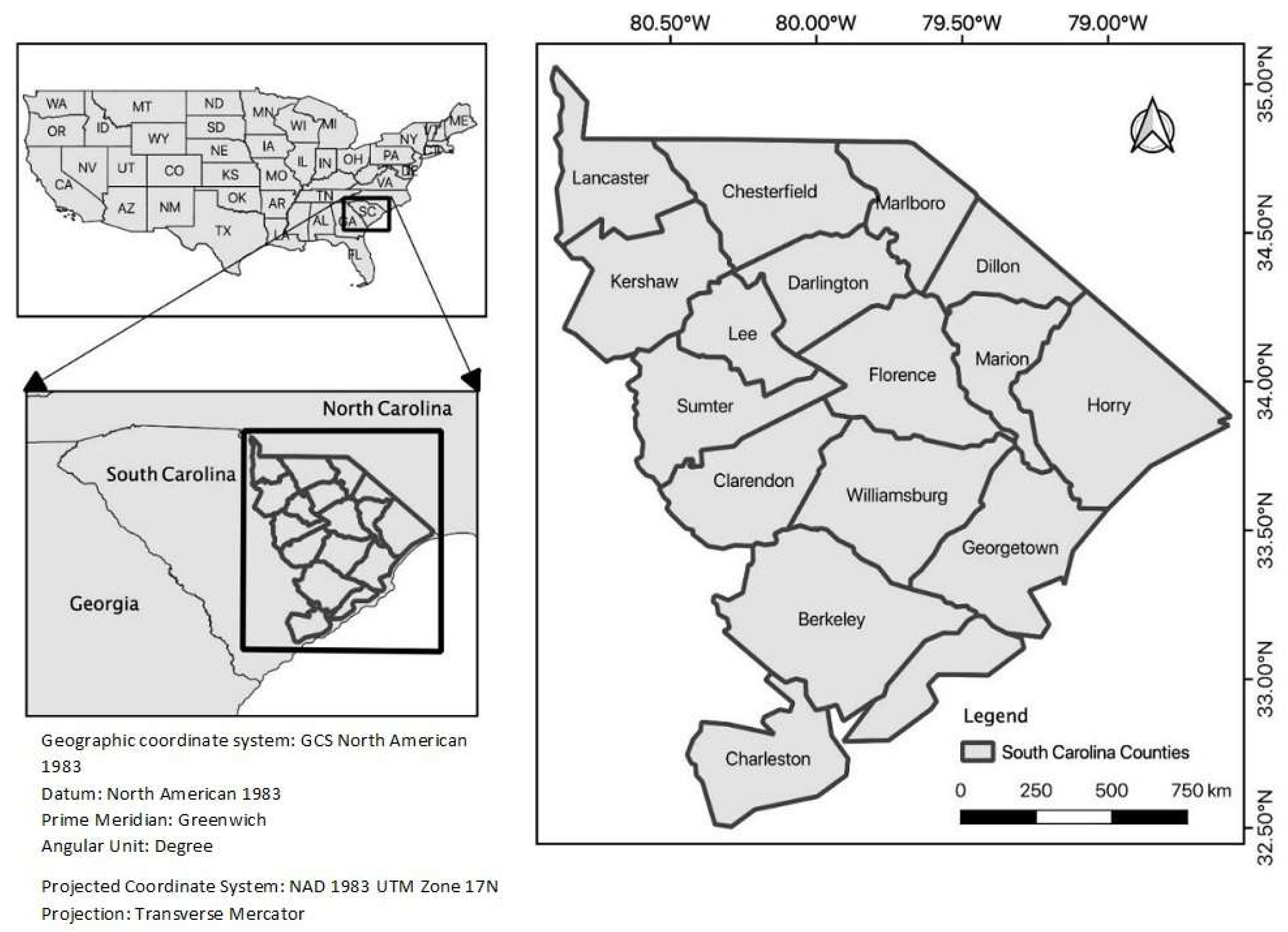
Figure 2.
A flow diagram for data processing and the analysis steps. Explains data processing and the analysis steps carried out in this study.
Figure 2.
A flow diagram for data processing and the analysis steps. Explains data processing and the analysis steps carried out in this study.
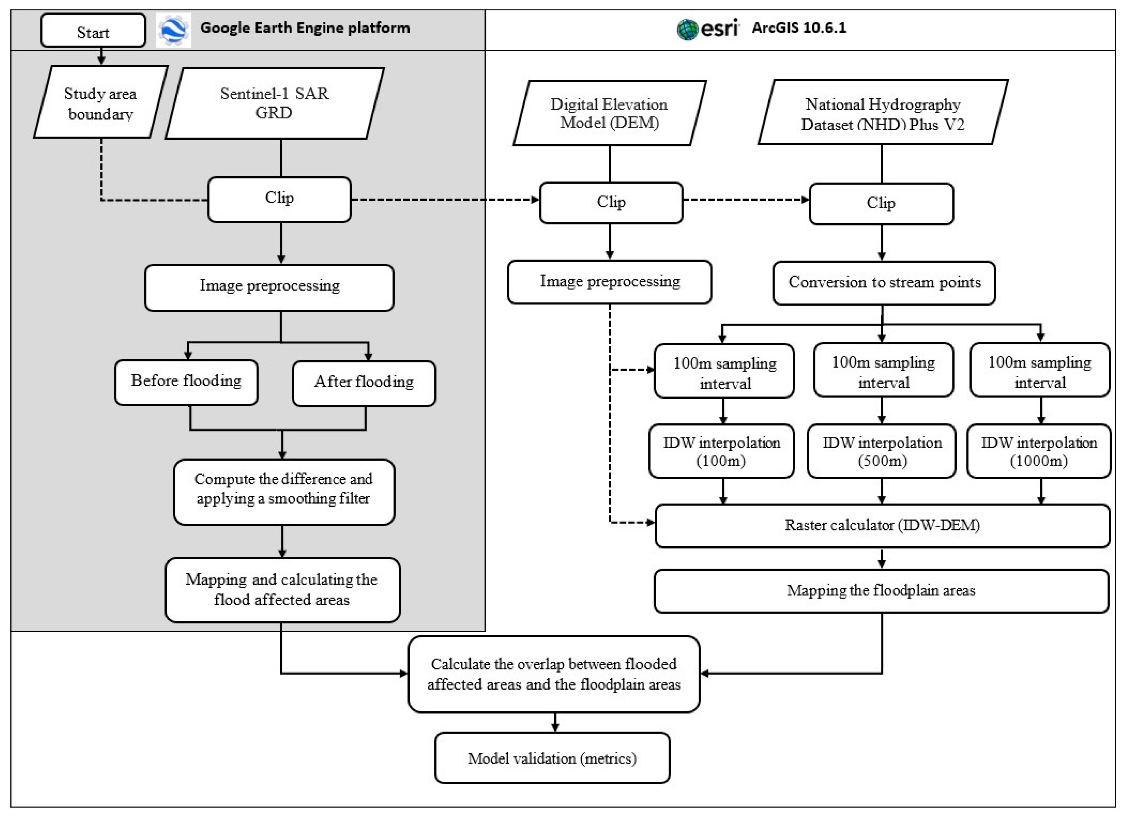
Figure 3.
Process of gathering sampling points used as data input for interpolation: (a) shows an overview of the points gathered within the stream across the landscape and (b) shows the different interval of sampling points which affects the accuracy of the interpolation.
Figure 3.
Process of gathering sampling points used as data input for interpolation: (a) shows an overview of the points gathered within the stream across the landscape and (b) shows the different interval of sampling points which affects the accuracy of the interpolation.
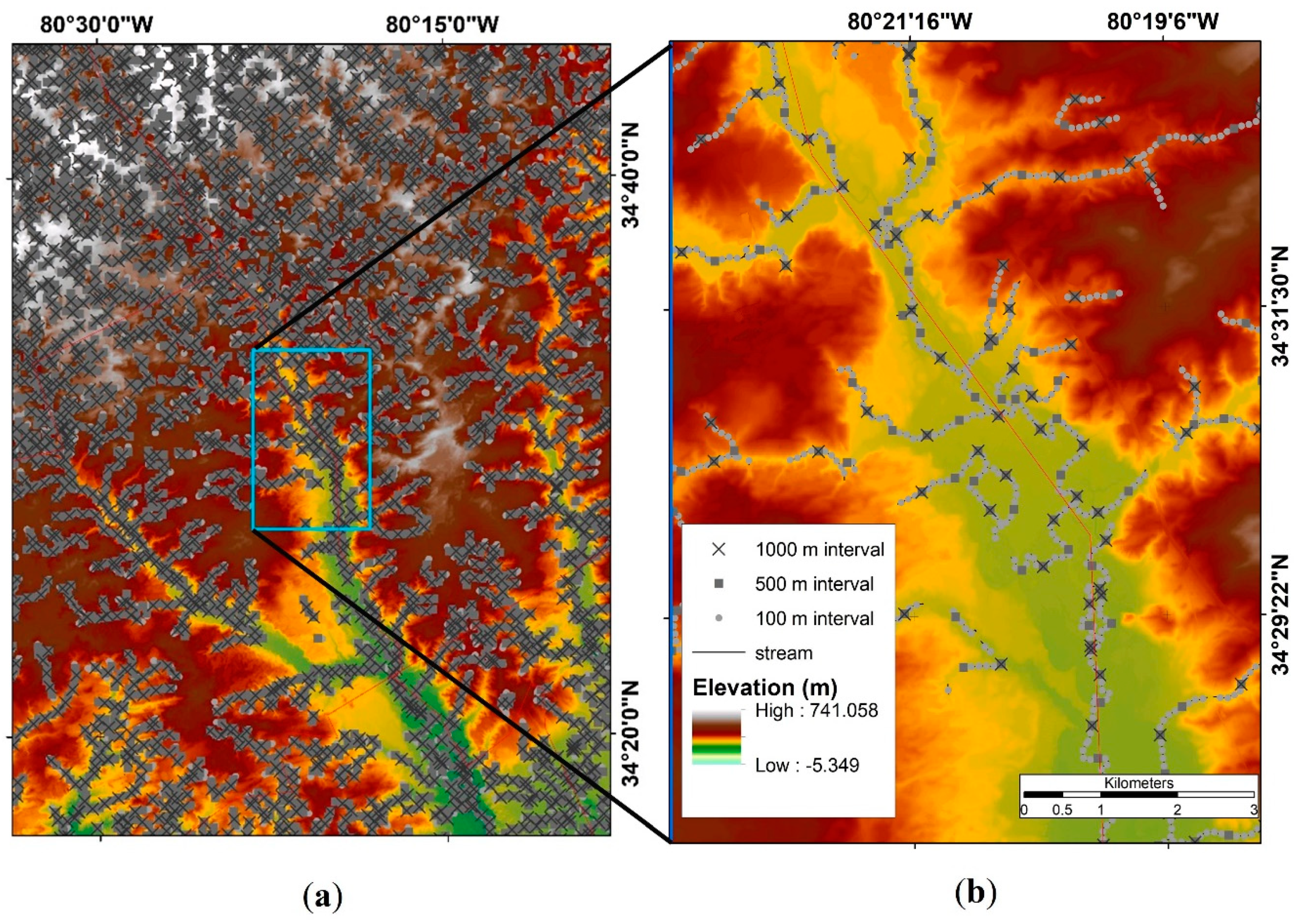
Figure 4.
ArcGIS model builder schematics for inverse distance weighting (IDW) generated floodplain.
Figure 4.
ArcGIS model builder schematics for inverse distance weighting (IDW) generated floodplain.
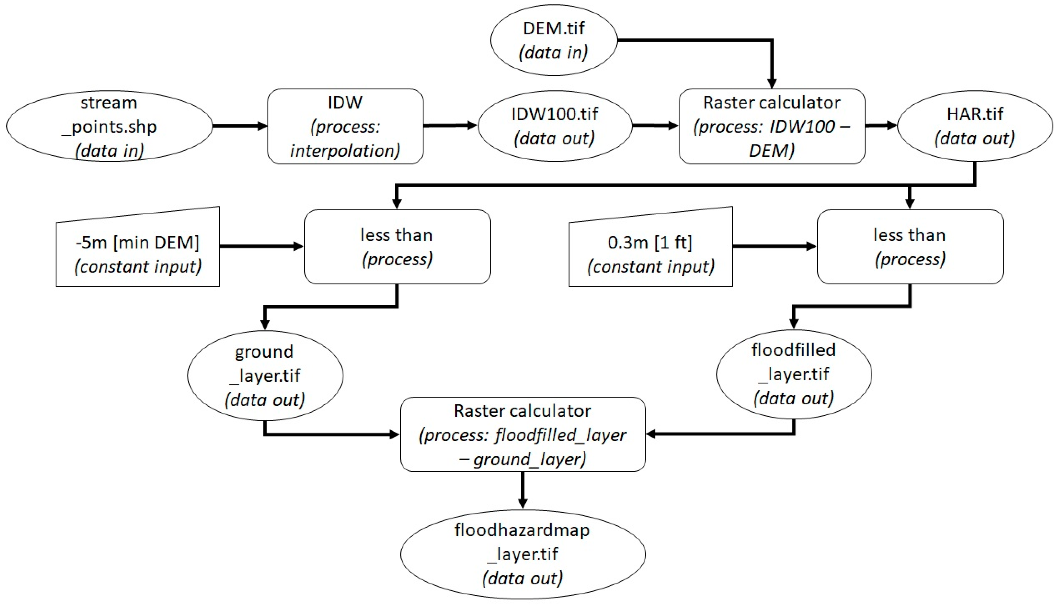
Figure 5.
Comparison between digital elevation models (DEM) and interpolated imagery: (a) shows Light Detection and Ranging (LiDAR)-based DEM with 3 m × 3 m resolution, (b) shows IDW result with default configuration [power = 2], and (c) shows IDW with optimized configuration [power = 39].
Figure 5.
Comparison between digital elevation models (DEM) and interpolated imagery: (a) shows Light Detection and Ranging (LiDAR)-based DEM with 3 m × 3 m resolution, (b) shows IDW result with default configuration [power = 2], and (c) shows IDW with optimized configuration [power = 39].

Figure 6.
Sampling sites (30 randomly selected sites from 100 Thiessen generated polygons) and application sites (10 selected coastal sites labeled A to J).
Figure 6.
Sampling sites (30 randomly selected sites from 100 Thiessen generated polygons) and application sites (10 selected coastal sites labeled A to J).

Figure 7.
Model results of IDW interpolation flood hazard area analysis: (a) shows the LiDAR-based DEM, which is the primary source of elevation points; (b) shows the geographic extent of the streams and hydrolines as source of the height above river (HAR); (c) shows the spatial distribution of flood hazard areas analyzed using an optimized configuration of IDW with 1000-m distance interval of sampling points within the stream; (d) a closer visualization of the sampling points within the streams; (e) shows how the flood hazard areas layout across the region while overlay with the predicted flood and the LiDAR-based DEM, and the black-shaded areas also show the intersect between the predicted floodplains and the flooded area; (f) shows a closer visualization of the flood hazard areas and how the streams and hydrolines have influenced the spatial distribution of flood hazard areas.
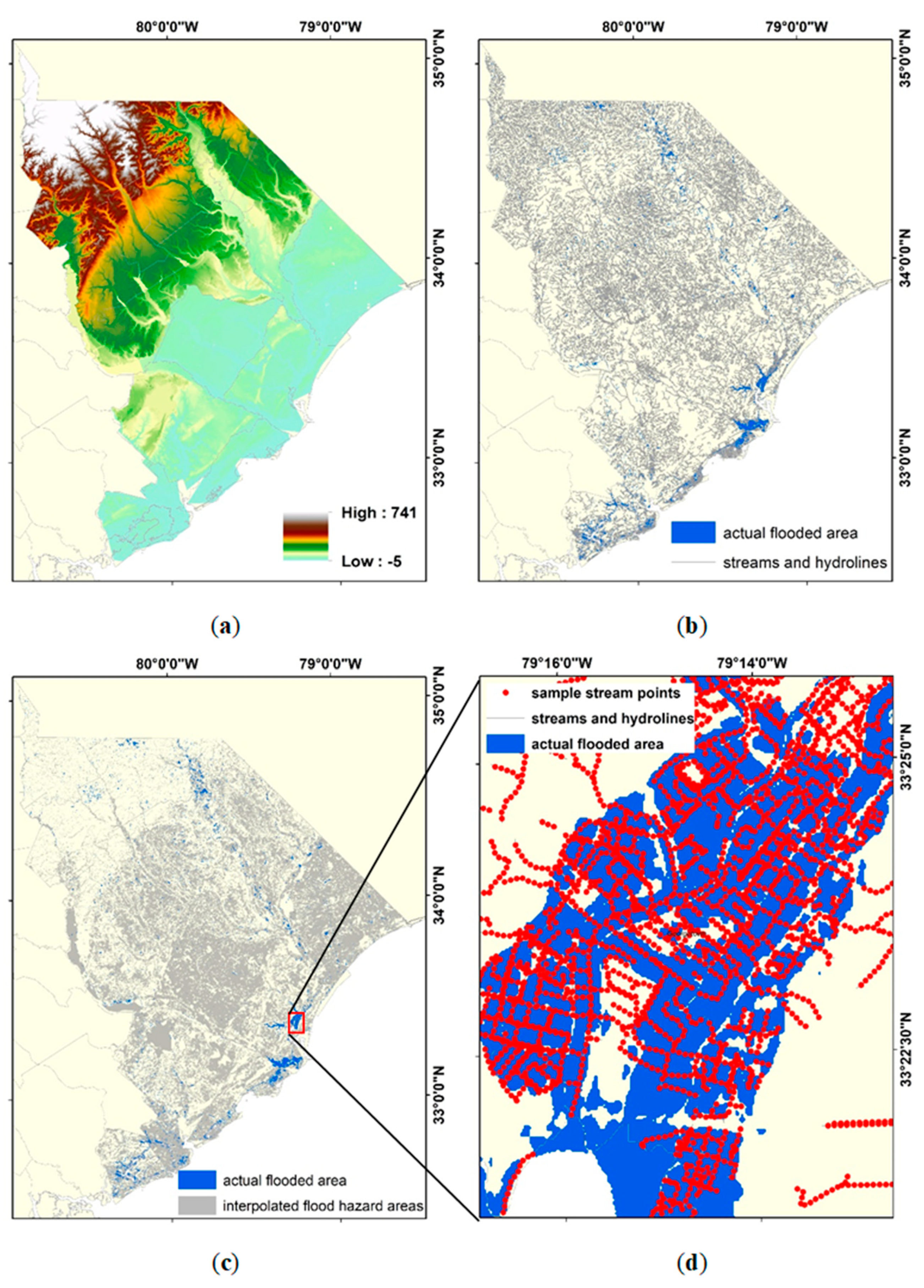

Figure 8.
Raster output of flood hazard area analysis: (a) shows specific sites locally selected from severely affected areas across the state; (b) results from Chesterfield, Marlboro, and Darlington counties; (c) results from Marion county, (d) results from Marion and Horry county; and (e) results from Georgetown county.
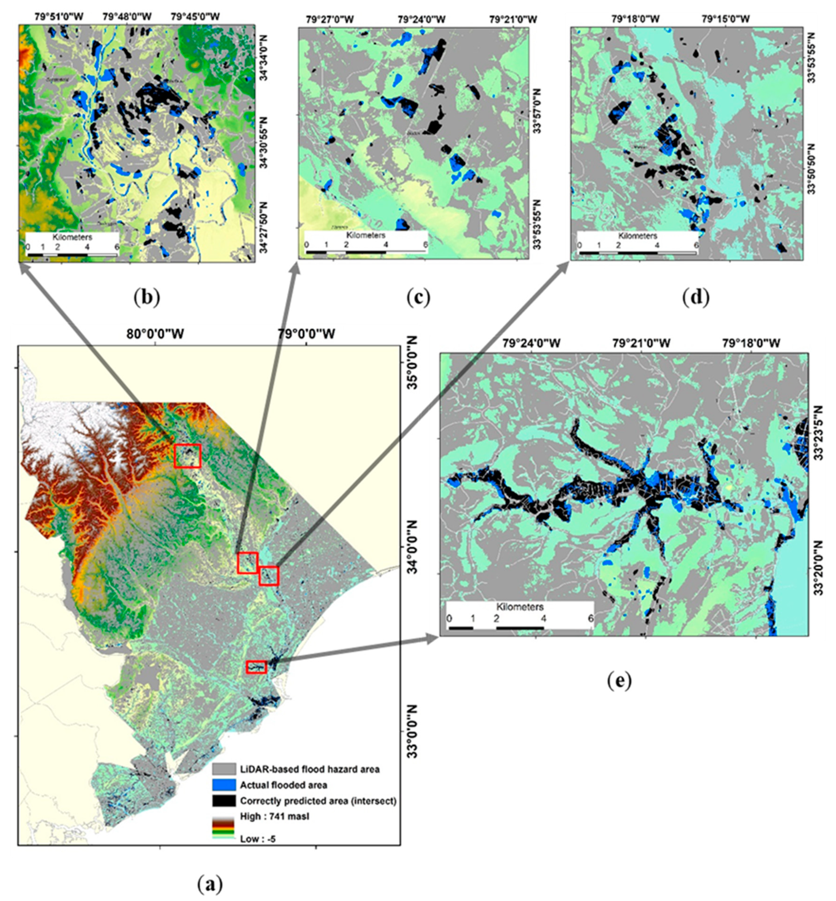
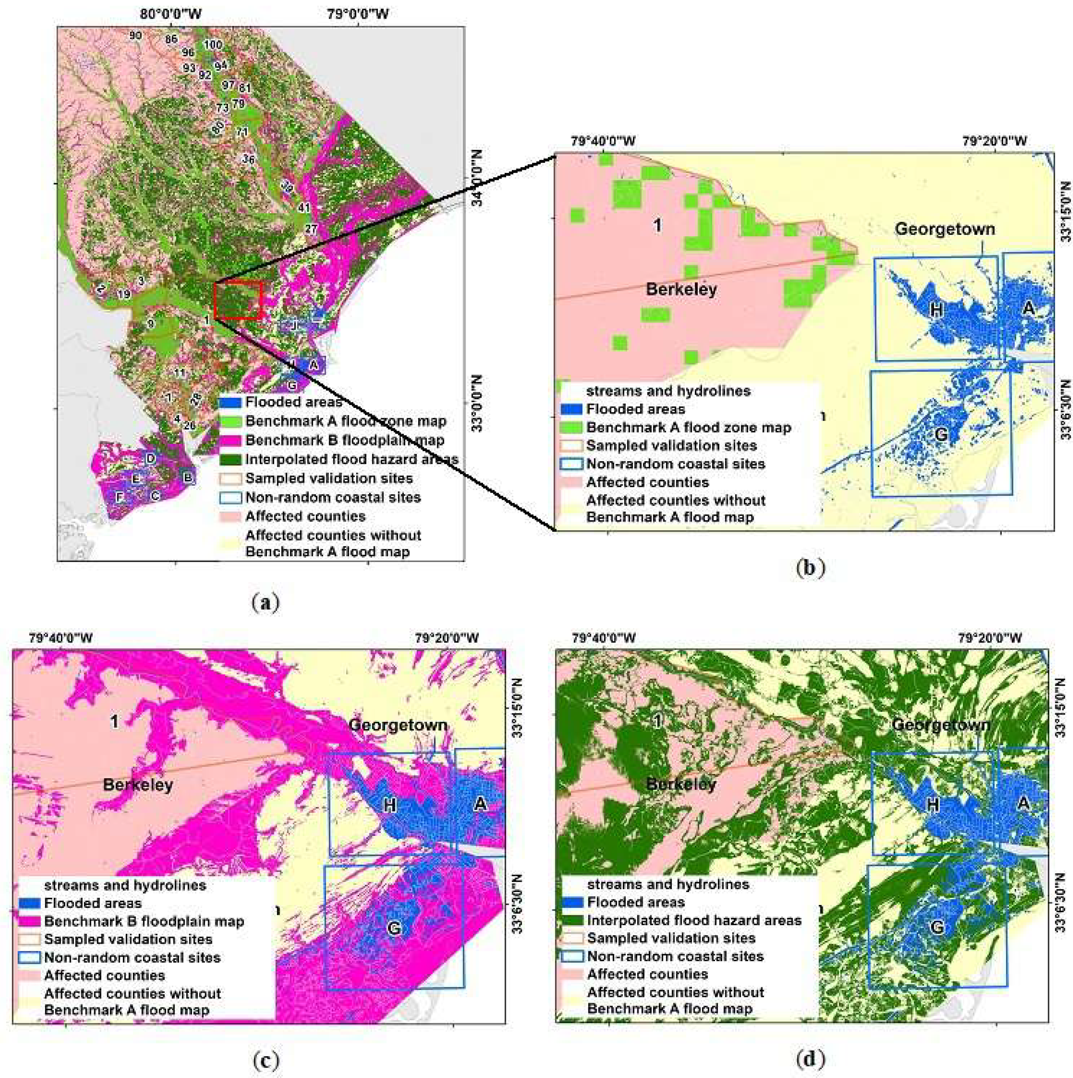
Figure 9.
Spatial distribution of benchmarks and interpolated flood hazard areas: (a) shows an overlay comparison of benchmark floodplains and flood hazard areas vis-à-vis the different model predicted flood hazard areas, (b) shows an overlay comparison of benchmark A flood hazard zones vis-à-vis the actual flooded areas, (c) shows an overlay comparison of benchmark B floodplain map vis-à-vis the actual flooded areas, and (d) shows an overlay of the model predicted flood hazard areas vis-à-vis the actual flooded areas.

Table 1.
Summary of model configurations and specification details for delineating floodplain.
| Configuration Name | Configuration Specifics | ||
|---|---|---|---|
| Stream Sampling Points Interval | DEM Source | IDW Configuration | |
| IDW100 | 100 m | LiDAR-based | Default (pval = 2) |
| IDW100opt | 100 m | LiDAR-based | Optimal (pval = 39) |
| IDW100_NED | 100 m | National Elevation Dataset | Default (pval = 2) |
| IDW100opt_NED | 100 m | National Elevation Dataset | Optimal (pval = 39) |
| IDW500 | 500 m | LiDAR-based | Default (pval = 2) |
| IDW500opt | 500 m | LiDAR-based | Optimal (pval = 39) |
| IDW500_NED | 500 m | National Elevation Dataset | Default (pval = 2) |
| IDW500opt_NED | 500 m | National Elevation Dataset | Optimal (pval = 39) |
| IDW1000 | 1000 m | LiDAR-based | Default (pval = 2) |
| IDW1000opt | 1000 m | LiDAR-based | Optimal (pval = 39) |
| IDW1000_NED | 1000 m | National Elevation Dataset | Default (pval = 2) |
| IDW1000opt_NED | 1000 m | National Elevation Dataset | Optimal (pval = 39) |
| Benchmark A | FEMA flood zone map from NFHL | ||
| Benchmark B | US EPA floodplain map by random forest (Woznicki et al. 2019) | ||
Table 2.
Mean and SD of % Fit in 30 sampled validation sites and 10 selected coastal sites.
| Model Configuration | 30 Sampled Areas Validated | 10 Coastal Sites Applied | ||
|---|---|---|---|---|
| Mean (%) | SD | Mean (%) | SD | |
| Benchmark A | 62 | 27 | – | – |
| Benchmark B | 66 | 26 | 97 | 3 |
| IDW100 | 50 | 15 | 69 | 16 |
| IDW100opt | 55 | 14 | 73 | 11 |
| IDW500 | 40 | 16 | 63 | 18 |
| IDW500opt | 51 | 14 | 69 | 13 |
| IDW1000 | 36 | 17 | 61 | 19 |
| IDW1000opt | 46 | 16 | 65 | 15 |
| IDW100_NED | 56 | 14 | 57 | 16 |
| IDW100opt_NED | 69 | 11 | 73 | 14 |
| IDW500_NED | 51 | 15 | 52 | 12 |
| IDW500opt_NED | 70 | 13 | 70 | 11 |
| IDW1000_NED | 50 | 14 | 49 | 13 |
| IDW1000opt_NED | 70 | 11 | 68 | 12 |
Table 3.
F-ratio summary statistics of 30 sampled validation sites and 10 selected coastal sites.
| Model Configuration | 30 Sampled Areas Validated | 10 Coastal Sites Applied | |||
|---|---|---|---|---|---|
| Mean (SD) | Test vs. Bmark A | Test vs. Bmark B | Mean (SD) | Test vs. Bmark B | |
| Benchmark A | −0.82 (0.11) | ||||
| Benchmark B | −0.84 (0.09) | 0.024 | −0.27 (0.25) | ||
| IDW100 | −0.85 (0.12) | 0.007 | 0.091 | −0.28 (0.26) | 0.403 |
| IDW100opt | −0.86 (0.12) | 0.001 | 0.032 | −0.31 (0.23) | 0.214 |
| IDW500 | −0.84 (0.13) | 0.123 | 0.490 | −0.25 (0.28) | 0.330 |
| IDW500opt | −0.85 (0.13) | 0.025 | 0.210 | −0.28 (0.24) | 0.432 |
| IDW1000 | −0.82 (0.14) | 0.432 | 0.178 | −0.23 (0.28) | 0.201 |
| IDW1000opt | −0.84 (0.14) | 0.143 | 0.483 | −0.25 (0.26) | 0.361 |
| IDW100_NED | −0.91 (0.08) | 0.000 | 0.000 | −0.37 (0.22) | 0.048 |
| IDW100opt_NED | −0.91 (0.07) | 0.000 | 0.000 | −0.39 (0.20) | 0.018 |
| IDW500_NED | −0.91 (0.08) | 0.000 | 0.000 | −0.38 (0.23) | 0.035 |
| IDW500opt_NED | −0.91 (0.07) | 0.000 | 0.000 | −0.39 (0.21) | 0.017 |
| IDW1000_NED | −0.91 (0.08) | 0.000 | 0.000 | −0.39 (0.23) | 0.047 |
| IDW1000opt_NED | −0.91 (0.07) | 0.000 | 0.000 | −0.38 (0.21) | 0.024 |
Table 4.
S-ratio summary statistics of 30 sampled validation sites and 10 selected coastal sites.
| Model Configuration | 30 Sampled Areas Validated | 10 Coastal Sites Applied | |
|---|---|---|---|
| vs. Bmark A | vs. Bmark B | vs. Bmark B | |
| Benchmark A | 1.00 | 0.85 | |
| Benchmark B | 1.15 | 1.00 | 1.00 |
| IDW100 | 1.20 | 1.13 | 0.72 |
| IDW100opt | 1.31 | 1.24 | 0.76 |
| IDW500 | 0.97 | 0.92 | 0.65 |
| IDW500opt | 1.23 | 1.16 | 0.71 |
| IDW1000 | 0.86 | 0.82 | 0.63 |
| IDW1000opt | 1.12 | 1.05 | 0.67 |
| IDW100_NED | 1.29 | 1.20 | 0.60 |
| IDW100opt_NED | 1.61 | 1.51 | 0.76 |
| IDW500_NED | 1.21 | 1.12 | 0.53 |
| IDW500opt_NED | 1.62 | 1.51 | 0.73 |
| IDW1000_NED | 1.21 | 1.14 | 0.51 |
| IDW1000opt_NED | 1.64 | 1.53 | 0.71 |
© 2020 by the authors. Licensee MDPI, Basel, Switzerland. This article is an open access article distributed under the terms and conditions of the Creative Commons Attribution (CC BY) license (http://creativecommons.org/licenses/by/4.0/).
Share and Cite
MDPI and ACS Style
Ureta, J.C.; Zurqani, H.A.; Post, C.J.; Ureta, J.; Motallebi, M. Application of Nonhydraulic Delineation Method of Flood Hazard Areas Using LiDAR-Based Data. Geosciences 2020, 10, 338. https://doi.org/10.3390/geosciences10090338
AMA Style
Ureta JC, Zurqani HA, Post CJ, Ureta J, Motallebi M. Application of Nonhydraulic Delineation Method of Flood Hazard Areas Using LiDAR-Based Data. Geosciences. 2020; 10(9):338. https://doi.org/10.3390/geosciences10090338
Chicago/Turabian StyleUreta, J. Carl, Hamdi A. Zurqani, Christopher J. Post, Joan Ureta, and Marzieh Motallebi. 2020. "Application of Nonhydraulic Delineation Method of Flood Hazard Areas Using LiDAR-Based Data" Geosciences 10, no. 9: 338. https://doi.org/10.3390/geosciences10090338
Note that from the first issue of 2016, this journal uses article numbers instead of page numbers. See further details here.