Article

Theoretical and Experimental Investigations of Identifying Bridge Damage Using Instantaneous Amplitude Squared Extracted from Vibration Responses of a Two-Axle Passing Vehicle

School of Civil Engineering, Guangzhou University, Guangzhou 510006, China
*
Authors to whom correspondence should be addressed.
Buildings 2024, 14(5), 1428; https://doi.org/10.3390/buildings14051428
Submission received: 1 April 2024 / Revised: 5 May 2024 / Accepted: 14 May 2024 / Published: 15 May 2024
(This article belongs to the Special Issue Advances in Research on Structural Dynamics and Health Monitoring)

Abstract

:
Identifying bridge damage using a movable test vehicle is highly regarded for its mobility, cost-effectiveness, and broad monitoring coverage. Previous studies have shown that the residual contact-point (CP) response between connected vehicles is free of the impact of vehicle self-vibrations and road roughness, making it particularly suitable for the indirect extraction of bridge modal properties. However, most experimental campaigns regarding contact-point (CP) responses focus on a single-axle testing vehicle within a non-moving state. This study aims to theoretically and experimentally identify bridge damage using the instantaneous amplitude squared (IAS) extracted from the residual CP response of a two-axle passing vehicle. First, the closed-form solution of the residual CP acceleration was derived for a two-axle vehicle interacting with a simply supported beam. The IAS index was constructed from the driving frequency of the residual CP acceleration. Then, numerical investigations using finite element simulation were conducted to validate using the IAS index for indirect bridge damage identification. The application scope of the approach under various vehicle speeds and road roughness grades was examined. Finally, a laboratory vehicle–bridge interaction system was tested to validate the approach. Numerical studies demonstrated that bridge damage could be directly determined by observing the IAS abnormalities, which were baseline-free. The IAS from the residual CP response outperformed the IAS from CP responses in identifying bridge damage. However, it was better to use the IAS when the vehicle speed was no greater than 2 m/s and the grade of the road surface roughness was not high. Laboratory tests showed that it was possible to identify bridge damage using the IAS extracted from the residual CP acceleration under perfect road surfaces. However, it fell short under rough road surfaces. Hence, further experiments are required to fully examine the capacity of the IAS for bridge damage identification in practical applications.

1. Introduction

Bridges, serving as vital infrastructural components enabling the traversal of terrain barriers, play a significant role in promoting regional economic development and facilitating social communication. However, bridges worldwide are aging, and the identification of damage in bridges has become a prominent focus in the field of structural health monitoring (SHM) [1,2]. Among all SHM methods, vibration-based methods constitute the primary research avenue for the identification of damage in bridges [3,4]. Traditional vibration monitoring involves placing sensors and data acquisition systems directly on the bridge to measure its dynamic responses. Subsequently, the vibrational signals are processed to facilitate the detection, localization, and quantification of bridge damage [1,2,3,4]. Given the extensive number of bridges and the limited lifespan of sensors, traditional direct vibration monitoring proves to be both costly and impractical for the health monitoring of a large bridge inventory. Hence, there is a continuous demand for more convenient and rapid structural health monitoring (SHM) methods for the health monitoring of existing bridge stocks.
Recently, a novel SHM paradigm involving the collection of vibration responses from passing vehicles to indirectly monitor bridges has been developing rapidly. This SHM paradigm is known as the vehicle scanning method (VSM), indirect monitoring, drive-by monitoring, vehicle-assisted method, or mobile sensing [5,6,7]. It is based on the vehicle–bridge interaction (VBI) mechanism wherein the bridge’s vibrations are transmitted to the passing vehicle, and processing the vibrational signal of the passing vehicle can identify the dynamic properties of the bridge. The VSM offers exceptional mobility, cost-effectiveness, and extensive detection coverage and eliminates the need for traffic disruptions, which is particularly suitable for assessing the health condition of numerous bridges. The initial VSM concept was proposed and validated in 2004 [8], but it has experienced significant development over the past five years [5,6,7]. This progress includes a substantial body of theoretical studies, numerical investigations, laboratory tests, and field measurements, covering the indirect measurements of bridge frequencies, mode shapes, damping ratios, road roughness, and damage. The identification of bridge frequencies using the VSM has been well-validated both in theory and experiments, and it has also found successful applications in engineering [9,10,11,12,13,14]. However, the application of the VSM in identifying bridge modal shapes and damage is primarily limited to theoretical investigations [15,16,17,18]. More recently, some laboratory tests on scaled VBI systems have attempted to fill this gap for validating the VSM in identifying bridge mode shapes and damage, but they are often conducted under ideal conditions [19,20,21,22]. The significant challenge in identifying bridge modal properties using the VSM arises from extracting weak bridge vibrational signals from vehicle responses amid the pollution caused by vehicle-induced vibrations and road surface roughness.
To mitigate the impact of vehicle vibrations, various filtering techniques have been employed to attenuate interference, including band-pass filters, variational modal decomposition, and particle filters [22]. However, these filtering processes strongly rely on the expertise of the signal processor, posing a risk of inadvertently filtering out the vibrational signals of the bridge. Some studies have introduced a tuned mass damper with its frequency tuned to the vehicle frequency to suppress vehicle self-vibrations, thereby mitigating the overall impact of vehicle-induced vibrations [23]. Moreover, design strategies involving specialized test vehicles with frequencies significantly isolated from vehicle frequencies through the use of large-axle stiffnesses have been proposed. These strategies have successfully enhanced the identification of bridge vibration signals from vehicle responses [24,25]. More recently, a novel approach to utilizing vehicle–bridge contact-point (CP) responses for extracting bridge dynamic properties has been introduced [26]. This strategy is advantageous because CP responses are inherently free from vehicle self-vibrations. To reduce the negative impact of road roughness, different strategies have been proposed, including using ongoing traffic, on-bridge shakers, and non-moving test vehicles [5,7]. However, these techniques usually require traffic restrictions, reducing the practical significance of the VSM for rapid bridge health monitoring under open traffic conditions. More recently, residual CP responses from two connected vehicles have been verified to be free from the influence of road surface roughness [18,27]. The potential implementation of residual CP responses in a two-axle vehicle is a fascinating prospect, achieved through a process of eliminating road surface roughness by subtracting the front and rear axle CP responses. While the theory behind this concept has been demonstrated, experimental validation is still required for practical application [28].
In the exploration of applying the VSM for indirect bridge damage identification, various studies have examined algorithms such as mode shape difference, wavelet transform, and deep learning [19,20,21,27]. Zhang et al. [26] introduced the metric of instantaneous amplitude squared (IAS), derived from the Hilbert transform of isolated bridge vibration signals from vehicle responses, to detect bridge damage. The spring-mass VBI model was employed in this study for illustration. Following this work, the feasibility of using the IAS for identifying bridge damage has been demonstrated using various numerical examples [16,27,28,29]; however, these studies lack experimental validation and do not consider more realistic road roughness conditions.
The objective of this study is to propose a VSM approach for identifying bridge damage using an IAS extracted from the residual CP responses of a two-axle passing vehicle with the consideration of road surface roughness. It fills the literature gap through the following two aspects. (1) It proposes an IAS metric extracted from residual CP responses of a two-axle passing vehicle, which simultaneously eliminates the negative influence of vehicle self-vibrations and road surface roughness. Currently, the IAS metric is derived from an oversimplified spring-mass vehicle model [26], which fails to mitigate the impact of road surface roughness. (2) It experimentally validates the utilization of the IAS and CP responses for indirect damage detection, an aspect that has not been addressed in current VSM studies, which predominantly focus on numerical validations. First, a closed-form solution for the VBI responses of a two-axle vehicle interacting with a simply supported beam was derived. Residual CP responses of the two-axle vehicle were derived and back-calculated from vehicle responses. An IAS metric was derived from the residual CP responses. Then, a numerical finite element simulation was prepared to validate theoretical derivations and verify the feasibility of the proposed VSM-based damage identification approach. Finally, laboratory tests were conducted to further validate the approach.

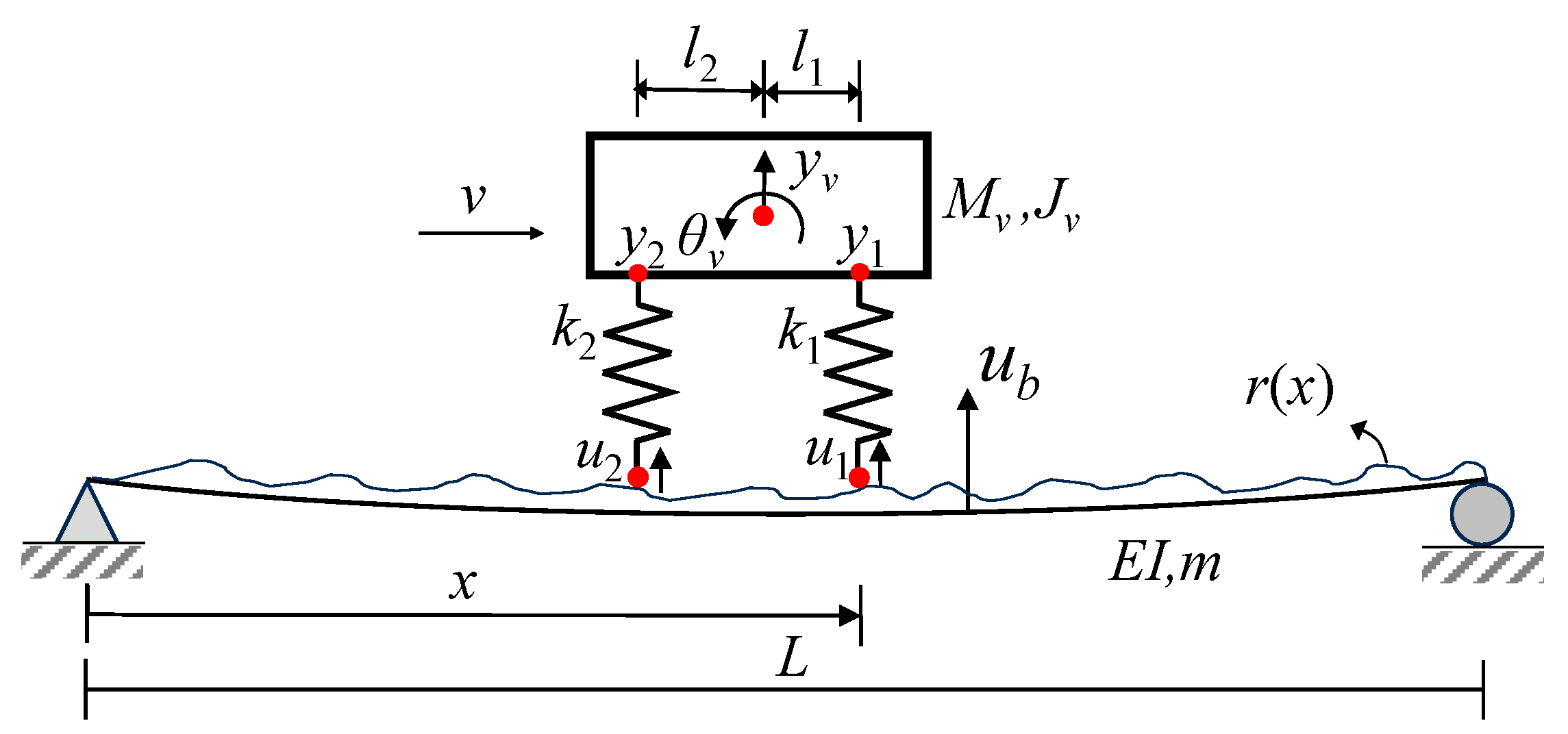
2. Theoretical Formulations of the Problem

In this section, the theoretical problem is presented by illustrating a two-axle vehicle interacting with a simply supported beam, as shown in Figure 1. The test vehicle is simplified to have two degrees of freedom of translational and rotational motions, i.e., yv and θv. These two degrees of freedom are functions of time. The main parameters of the simply supported beam consist of the bridge length L, mass per unit length m, elastic modulus E, and moment of inertia I. The parameter EI is the bending rigidity of the beam. The main parameters of the two-axle vehicle comprise the vehicle mass Mv and mass moment of inertia of the vehicle Jv. The front and rear axle spring stiffness are k1 and k2, and the distance from the front and rear wheels to the center of gravity of the vehicle are l1 and l2, respectively. The vehicle passes over the bridge at a constant speed of v. In the following study, the closed-form solutions for the CP responses of the test vehicle passing over the simply supported beam are first derived. Then, the residual CP responses are obtained by subtracting the time-lagged CP response of the front axle from the CP response of the rear axle. Finally, the IAS index, which can reflect damage location, is formulated based on the Hilbert transform of the drive frequency response components of the residual CP responses.
The assumptions used for theoretical formulations are summarized as follows: (1) The simply supported beam is the Euler–Bernoulli type with a constant cross-section, where the shear deformation and rotary inertia are not considered. (2) The damping of the system and bridge road roughness are not considered. (3) The vehicle mass is assumed to be significantly less than the bridge mass, and its influence on bridge modal properties is ignored. (4) The velocity of the vehicle remains constant during its passage. (5) The vehicle–bridge coupled interaction is ignored in solving bridge responses but considered in deriving vehicle responses. These assumptions are commonly adopted in VSM studies [5,6,7,8,9,10,11,12,13,14,15,16,17,18,19,20,21,22,23,24,25,26,27,28,29] for theoretical derivation. Nevertheless, the full interactions of the moving vehicle with the beam, the consideration of the shear deformation and rotary inertia of the beam, damping, and non-constant vehicle velocity are meaningful for follow-up works [30,31].

2.1. Closed-Form Solutions of Residual CP Responses

To streamline the formulation, the vehicle mass is generally considered to be negligible with respect to the bridge, and thus, the vehicle–bridge coupling effect can be ignored. This assumption is frequently adopted in VSM studies [5,6,7], yet its validity may be questionable and warrants closer consideration when investigating the coupling effects [32]. Nevertheless, the vehicle–bridge coupling effects will be fully considered in the following numerical examples. Hence, the two-axle vehicle passing over the bridge can be regarded as two moving forces acting on the bridge, and the close-from solution of the bridge displacement ub can be obtained as follows [22]:
u b ( x , t ) = n = 1 N k = 1 2 q k ( t ) sin ( n π x L ) ,
where
q k ( t ) = 2 L 3 ( l l k ) M v g E I n 4 π 4 l ( 1 S n 2 ) { [ sin ( n π v ( t t k ) L ) S n sin ( ω b n ( t t k ) ) ] H ( t t k ) + [ sin ( n π v ( t t k Δ t ) L ) S n sin ( ω b n ( t t k Δ t ) ) ] H ( t t k Δ t ) } ,
where H (·) represents the unit step function, tk = (l1 + l2)(k − 1)/v represents the entry time of the kth vehicle axle into the beam (k = 1, 2), and Δt = L/v denotes the time duration of the vehicle axle staying on the bridge. Moreover, ωbn denotes the nth bridge frequency, and Sn denotes the speed parameter, which can be expressed as follows:
ω b n = n 2 π 2 L 2 E I m , S n = n π v L ω b n .
Furthermore, the vehicle is considered to be symmetric, i.e., k1 = k2 = k, l1 = l2 = l. This assumption is solely for the convenience of theoretical derivations and does not affect the proposed approach. Additionally, many real-world two-axle vehicles can be considered symmetric, such as train carriages. Let x = v(ttk), and the CP displacement of the kth axle uk(t) at the timestamp t is the superposition of the CP displacement of the bridge u b (x,t)|x=vt. The road surface roughness r(x)| x=vt, given as follows:
u i ( t ) = n = 1 N k = 1 2 A n { cos n π v ( t k t i ) L cos ( 2 n π v t L n π v ( t k + t i ) L ) + S n cos ( ( ω b n + n π v L ) t ω b n t k n π v t i L ) S n cos ( ( ω b n n π v L ) t ω b n t k + n π v t i L ) } × [ H ( t t k ) H ( t t k Δ t ) ] + r ( x ) |   x = v t , ( i = 1 , 2 ) ,
where
A n = L 3 M v g 2 E I n 4 π 4 ( 1 S n 2 ) .
It is shown in Equations (2) and (4) that the CP response of the vehicle axle contains four components: road surface roughness r, the driving frequency 2nπv/L, the left-shifted bridge frequencies ωbnnπv/L, and the right-shifted bridge frequencies ωbn + nπv/L. The CP response excludes the component of vehicle frequency but is influenced by the road surface roughness. Notably, road roughness is a broadband signal that obscures all frequency components, posing challenges in extracting bridge frequencies from the CP response.
However, the information on road surface roughness is presented in the CP responses of the front and rear axles at different moments, i.e., t and t − d/v. Therefore, the influence of the road surface roughness can be eliminated by subtracting the time-lagged CP response of the rear axle from the CP response of the front axle. In the following study, the driving frequency component and the road roughness component in Equation (3) are selected for further derivation. To simplify the theoretical derivation, the unit step function component H (·) in Equation (4) is treated as 1, i.e., the vehicle axles are always in contact with the bridge. Therefore, the Equation (4) can be rewritten as follows:
{ u 1 ( t ) = { n = 1 N A n [ cos ( 2 n π v t L ) + cos ( 2 n π v t L 2 n π l L ) ] } + r ( x ) | x = v t + B 1 u 2 ( t ) = { n = 1 N A n [ cos ( 2 n π v t L 2 n π l L ) + cos ( 2 n π v t L 4 n π l L ) ] } + r ( x ) | x = v ( t t 2 ) + B 2 ,
where
{ B 1 = n = 1 N A n [ cos ( 2 n π l L ) + S n cos ( ω b n + n π v L ) t cos ( ( ω b n + n π v L ) t 2 l ω b n v ) S n cos ( ω b n n π v L ) t cos ( ( ω b n n π v L ) t 2 l ω b n v ) ] B 2 = n = 1 N A n [ cos ( 2 n π l L ) + S n cos ( ( ω b n + n π v L ) t 2 n π l L ) cos ( ( ω b n + n π v L ) t 2 n π l L 2 l ω b n v ) S n cos ( ( ω b n n π v L ) t + 2 n π l L ) cos ( ( ω b n n π v L ) t + 2 n π l L 2 l ω b n v ) ] .
When introducing a time lag of 2l/v to the CP displacement of the rear axle, u2(t) is rewritten as follows:
u 2 ( t + 2 l v ) = { n N A n [ cos ( 2 n π v t L ) + cos ( 2 n π v t L + 2 n π l L ) ] } + r ( x ) | x = v t + B ˜ 2 ,
where
B ˜ 2 = n N A n [ cos ( 2 n π l L ) + S n cos ( ( ω b n + n π v L ) t + 2 l ω b n v ) cos ( ω b n + n π v L ) t S n cos ( ( ω b n n π v L ) t + 2 l ω b n v ) cos ( ω b n n π v L ) t ] .
Following the CP displacement of the front axle in Equation (6) and the CP displacement of the rear axle in Equation (8), the residual CP displacement is obtained as follows:
Δ u = u 2 ( t + 2 l v ) u 1 ( t ) = { n N A n [ cos ( 2 n π v t L + 2 n π l L ) cos ( 2 n π v t L 2 n π l L ) ] } + B ˜ ,
where
B ˜ = n N A n [ 2 cos ( 2 n π l L ) + S n cos ( ( ω b n + n π v L ) t + 2 l ω b n v ) cos ( ω b n + n π v L ) t S n cos ( ( ω b n n π v L ) t + 2 l ω b n v ) cos ( ω b n n π v L ) t S n cos ( ω b n + n π v L ) t cos ( ( ω b n + n π v L ) t 2 l ω b n v ) + S n cos ( ω b n n π v L ) t cos ( ( ω b n n π v L ) t 2 l ω b n v ) ] .
It is shown in Equation (10) that the influence of the road surface roughness was removed from the residual CP displacement. Only the frequency components of the driving frequency 2nπv/L and the left-shifted and right-shifted bridge frequencies B ˜ are retained. Considering that the acceleration is easier than the displacement for field measurements, Equation (10) is differentiated twice, and the residual CP acceleration is obtained as follows:
Δ u ¨ = { n = 1 N 4 n 2 π 2 v 2 A n L 2 [ cos ( 2 n π v t L 2 n π l L ) cos ( 2 n π v t L + 2 n π l L ) ] } + B ¨ ˜ ,
where B ¨ ˜ is the second time derivative of Equation (11).
Notably, the CP acceleration of the vehicle axles described above cannot be directly measured. This is because the above closed-form solutions require prior knowledge of the modal information of the bridge, which is what the VSM seeks to identify. However, the axle responses can be indirectly back-calculated from the vehicle responses, which are formulated as follows [26,27]:
{ u 1 ( t ) = M v l 2 + J v 4 k l 2 y ¨ 1 ( t ) + M v l 2 J v 4 k l 2 y ¨ 2 ( t ) + y 1 ( t ) u 2 ( t ) = M v l 2 J v 4 k l 2 y ¨ 1 ( t ) + M v l 2 + J v 4 k l 2 y ¨ 2 ( t ) + y 2 ( t ) ,
where y1 and y2 are the vertical displacements of the vehicle body at the front and rear axles, as illustrated in Figure 1.
By substituting Equation (13) into Equation (10), the residual CP displacement can be obtained as follows:
Δ u = u 2 ( t + 2 l v ) u 1 ( t ) = [ M v l 2 J v 4 k l 2 y ¨ 1 ( t + 2 l v ) + M v l 2 + J v 4 k l 2 y ¨ 2 ( t + 2 l v ) + y 2 ( t + 2 l v ) ] [ M v l 2 + J v 4 k l 2 y ¨ 1 ( t ) + M v l 2 J v 4 k l 2 y ¨ 2 ( t ) + y 1 ( t ) ] .
Furthermore, the residual CP acceleration can be formulated by differentiating Equation (14) twice, given as follows:
Δ u ¨ = u ¨ 2 ( t + 2 l v ) u ¨ 1 ( t ) = [ M v l 2 J v 4 k l 2 d 2 y ¨ 1 ( t + 2 l v ) d t 2 + M v l 2 + J v 4 k l 2 d 2 y ¨ 2 ( t + 2 l v ) d t 2 + y ¨ 2 ( t + 2 l v ) ] [ M v l 2 + J v 4 k l 2 d 2 y ¨ 1 ( t ) d t 2 + M v l 2 J v 4 k l 2 d 2 y ¨ 2 ( t ) d t 2 + y ¨ 1 ( t ) ] .
Therefore, it is known that the residual CP acceleration of the two-axle passing vehicle can be calculated from the vehicle responses y ¨ 1 and y ¨ 2, which are practical for measurements. Notably, the above derivations ignore the vehicle–bridge coupled effect, which will be investigated in the following numerical validation section.

2.2. Bridge Damage Detection Using Residual CP Acceleration

In this section, the driving frequency component (2nπv/L) from the residual CP acceleration of the two-axle passing vehicle is isolated to construct the IAS for identifying bridge damage. The rationale for selecting driving frequencies rather than bridge frequencies is their low and closely distributed nature, which reduces the likelihood of contamination by high-frequency signals such as environmental noise and road roughness signals. After applying the fast Fourier transform (FFT) to the residual CP acceleration in Equation (12), the corresponding frequency spectrum is formulated as follows:
F ( ω ) = Δ u ¨ ( t ) e j ω t d t .
The components of driving frequencies in Equation (12) can be isolated from the residual CP acceleration by applying a multi-peak spectrum idealized filter as follows:
H d ( ω ) = { 1 ω = 2 n π v / L 0 e l s e .
By applying the idealized filter transfer function to the frequency function of the residual CP acceleration, the filtered amplitude frequency function is obtained as follows:
F d ( ω ) = F ( ω ) × | H d ( ω ) | = Δ u ¨ ( t ) e j ω t d t ,   ω = 2 n π v / L .
Then, the time-domain response of Fd(jw) can be reconstructed using inverse FFT as follows:
R n ( t ) = 1 2 π F d ( ω ) e j ω t d ω = n = 1 N D n [ cos ( 2 n π v t L 2 n π l L ) cos ( 2 n π v t L + 2 n π l L ) ] ,
where
D n = 4 n 2 π 2 v 2 A n L 2 .
Therefore, the driving frequency components Rn(t) in the time domain are extracted from the residual CP acceleration. The driving frequency component responses are narrowband time series, and the Hilbert transform can be applied to obtain its pair. Consequently, the Hilbert transform of Rn(t) is derived as follows:
R n ( t ) = n = 1 N D n [ sin ( 2 n π v t L 2 n π l L ) sin ( 2 n π v t L + 2 n π l L ) ] .
According to Equations (19) and (21), the IAS index can be constructed as follows:
A 2 ( t ) = R n 2 ( t ) + R n 2 ( t ) = 2 ( n = 1 N D n 2 j = 1 N i = 1 N D j D i cos 2 π l ( j + i ) L ) + 4 j = 1 N i = 1 ( i > j ) N D j D i [ ( 1 2 sin 2 π v t ( j i ) L ) ( cos 2 π l ( j i ) L cos 2 π l ( j + i ) L ) ] .
It is acknowledged that the mode shape of the bridge for the simply supported beam is Φ = sin n π v t / L . By substituting the mode shape function into Equation (22), the relationship between the IAS and the bridge mode shape Φ is expressed as follows:
IAS = A 2 ( t ) = 2 ( n = 1 N D n 2 j = 1 N i = 1 N D j D i cos 2 π l ( j + i ) L ) + 4 j = 1 N i = 1 ( i > j ) N D j D i [ ( 1 2 Φ j i 2 ) ( cos 2 π l ( j i ) L cos 2 π l ( j + i ) L ) ] ,
It is shown in the equation that the IAS index is closely connected with the bridge mode shape Φ. It is widely understood that the presence of damage alters the bridge mode shape. This suggests that the IAS can reflect the bridge damage because the bridge mode shape Φ will be changed if damage occurs in the beam. Therefore, the IAS index can detect the existence and location of damage. Concerning the severity of the damage, the abnormality level of the IAS index can capture this severity. Therefore, the following practical procedures are proposed for identifying bridge damage using the IAS extracted from the residual CP acceleration, as follows:
  • Measure the vehicle accelerations y ¨ 1 and y ¨ 2 of the vehicle body at the front and rear axles of the two-axle test vehicle;
  • Calculate the residual CP acceleration Δ u ¨ of the front and rear vehicle axles using Equation (15);
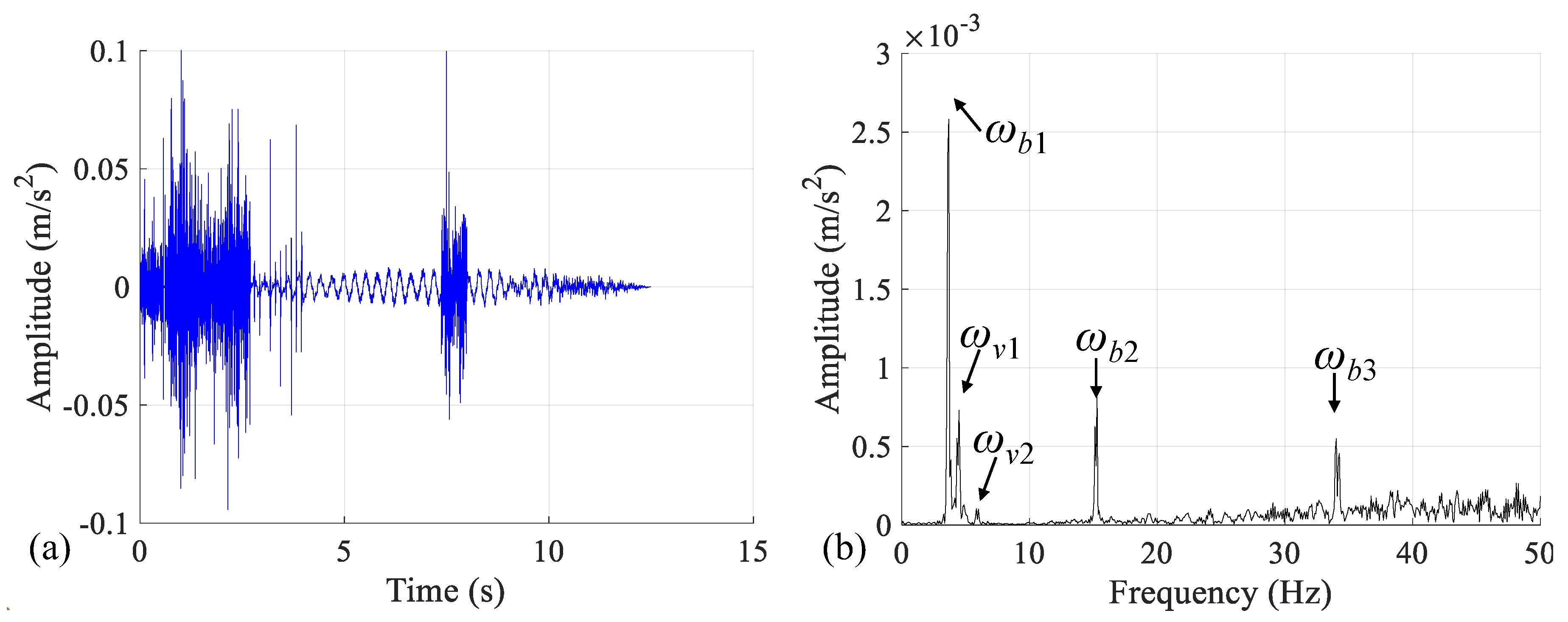
  • Analyze the frequency spectrum of Δ u ¨ using FFT and isolate its first few orders of driving frequencies 2nπv/L using the multi-peak spectrum idealized filter;
  • Obtain the time-domain results of the driving frequency components Rn(t) using the multi-point spectra idealized filter and inverse FFT and construct its instantaneous amplitude IAS index A(t) by Hilbert transform.

3. Numerical Investigations Using Finite Element Simulation

3.1. Finite Element Simulation of the VBI System with Damage

In this section, the finite element simulation is conducted for a symmetric two-axle vehicle interacting with a simply supported beam (see Figure 2). The bridge is divided into Ne beam units with an equal length Le. The beam element has two nodes, each considering two degrees of freedom, i.e., nodding and sinking. The beam element where the vehicle axle acts is a new VBI element as it considers both the motion of the beam element and the vehicle. The equations of motion of the VBI element and normal beam element are provided in [22,30]. The vehicle axle distance d = (l1 + l2) must be larger than the length of the beam element Le to ensure each vehicle axle acts on different beam elements. Furthermore, to facilitate the following discussions regarding vehicle damping and stiffness, a distinction is made between damping and stiffness of the front and rear axles using subscripts 1 and 2.
In addition, the beam damage is considered as the loss of element stiffness [33]. Notably, damage in beam-like structures can also be modeled in other forms, such as cracks or internal hinges [33,34]. However, the reduction in element stiffness remains the most common technique of damage modeling. Additionally, this study does not concentrate on modeling and detecting beam damage at the meso scale, including pinpointing the damage location or determining the damage direction within the beam cross-section. This study’s objectives revolve around detecting and quantifying damage in field applications, with no emphasis on damage quantification at the meso scale. The following simple theoretical derivation is employed to illustrate that the decrease in structural stiffness directly causes a change in the modal vibration pattern of the bridge. For the undamped, freely vibrating beam, the characteristic equation of dynamics is as follows:
( K λ M ) Φ = 0 ,
where K and M represent the structural stiffness and mass matrices, and λ and Φ denote the structural eigenvalues and eigenvectors, respectively.
Assuming that the beam experiences an element stiffness loss, and ignoring the change in beam mass resulting from the element stiffness loss, the characteristic equation of dynamics is as follows:
[ ( K + Δ K ) ( λ + Δ λ ) M ] ( Φ + Δ Φ ) = 0 ,
where ΔK denotes the change in structural element stiffness, and Δλ and ΔΦ denote the change of the structural eigenvalue and the change of the structural eigenvector, respectively. By left-multiplying the ΦT on both sides of Equation (15), the change in structural eigenvalue can be expressed as follows:
Δ λ = Φ T Δ K ( Φ + Δ Φ ) Φ T M ( Φ + Δ Φ ) .
Clearly, the presence of element stiffness loss directly affects the eigenfrequencies and eigenvectors. Since the IAS index is closely related to the eigenvectors, it can be used to locate and quantify the beam damage.

3.2. Numerical Validation of the Residual CP Response

A numerical example with the vehicle and bridge parameters, outlined in Table 1, is investigated. These vehicle and bridge parameters are strictly selected to reflect the realistic conditions of highway bridges, consistent with widely accepted practices in VSM studies [8,10,12,16,22,23,26]. Notably, the parameter values remain constant in the following investigations unless otherwise noted. The simply supported bridge was divided into 50 elements, and the time step of the finite element simulation was 0.001 s. The number of beam elements plays a pivotal role in the VBI responses within the numerical investigation of damage. This is because the size of the damage is equated to the element size for modeling damage through element stiffness loss. In this study, the chosen size for the damaged element is 0.5 m, a dimension commonly employed in the literature [10,11,12,13,14,15,16,17,18,19,20,21,22,23,24,25,26,27,28]. Consequently, a total of 50 elements constitute the 25 m simply supported beam. In addition, a simulation time step of 0.001 s is also a common choice in VBI studies [10,11,12,13,14,15,16,17,18,19,20,21,22,23,24,25,26,27,28]. The first third frequencies of the bridge are ωb1 = 3.80 Hz, ωb2 = 15.22 Hz, and ωb3 = 34.24 Hz, respectively. The frequencies of the test vehicle are ωv = 4.35 Hz and ωθ = 5.96 Hz. The road is assumed to have a relatively smooth surface with Gd(n0) = 0.001 × 10⁻⁶ m3 [22]. To be consistent with the theoretical analysis, the bridge and vehicle damping are not considered. However, the vehicle in the numerical example is considered to be asymmetric for a general case.
Three methods were employed to calculate the CP displacements. The first method involves directly interpolating using the displacement responses of adjacent beam nodes based on the location of the wheel contact points in the beam element, referred to as FEM-B, which is the most accurate calculation result. The second method is back-calculating from the vehicle responses using Equation (13), referred to as FEM-V, which may be biased owing to the introduction of numerical differencing. The third method is the theoretical calculation by substituting x = vt into Equation (1), referred to as “Analytical,” which may be biased because it ignores the vehicle–bridge coupled interaction and considers only the first five bridge frequencies. Notably, the consideration of the first five modes of modal information for theoretical VBI analysis is a common choice in the literature [10,14,17,22,31]. The comparison of the CP response at the front axle of a two-axle vehicle calculated by the three methods is provided in Figure 3. Notably, the contact point displacement is the sum of road surface roughness and bridge displacement, as shown in Equation (4). It is shown in Figure 3a that the three methods yield consistent CP displacements, which validate the correctness of the theoretical derivation and numerical modeling. Slight deviations are observed in the results of “Analytical,” owing to the ignorance of the VBI coupling effect. As can be seen in Figure 3b, only the first bridge frequency can be extracted from the spectrum of the CP acceleration at the front axle, owing to the interference of the road surface roughness. Again, as before, the spectrum of the CP acceleration calculated by the three methods yields the same results.
The influence of road surface roughness can be eliminated by using the residual CP response, according to Equation (10). Therefore, the residual CP response of the two-axle test vehicle back-calculated from the vehicle responses is provided in Figure 4. As shown in Figure 4b, the high-frequency spectra exhibit a greater complexity compared to the low-frequency spectra, owing to the anomalous vibrations shown in Figure 4a. Nevertheless, the first three bridge frequencies are still visible and easy to identify in the frequency spectra, which suggests that the residual CP responses eliminate the interference of the road surface roughness. In addition, it should be noted that the frequencies of the vehicle are also found in the spectrum of residual CP acceleration, which can be attributed to the presence of road surface roughness that renders the vehicle–bridge coupling impossible to overlook.

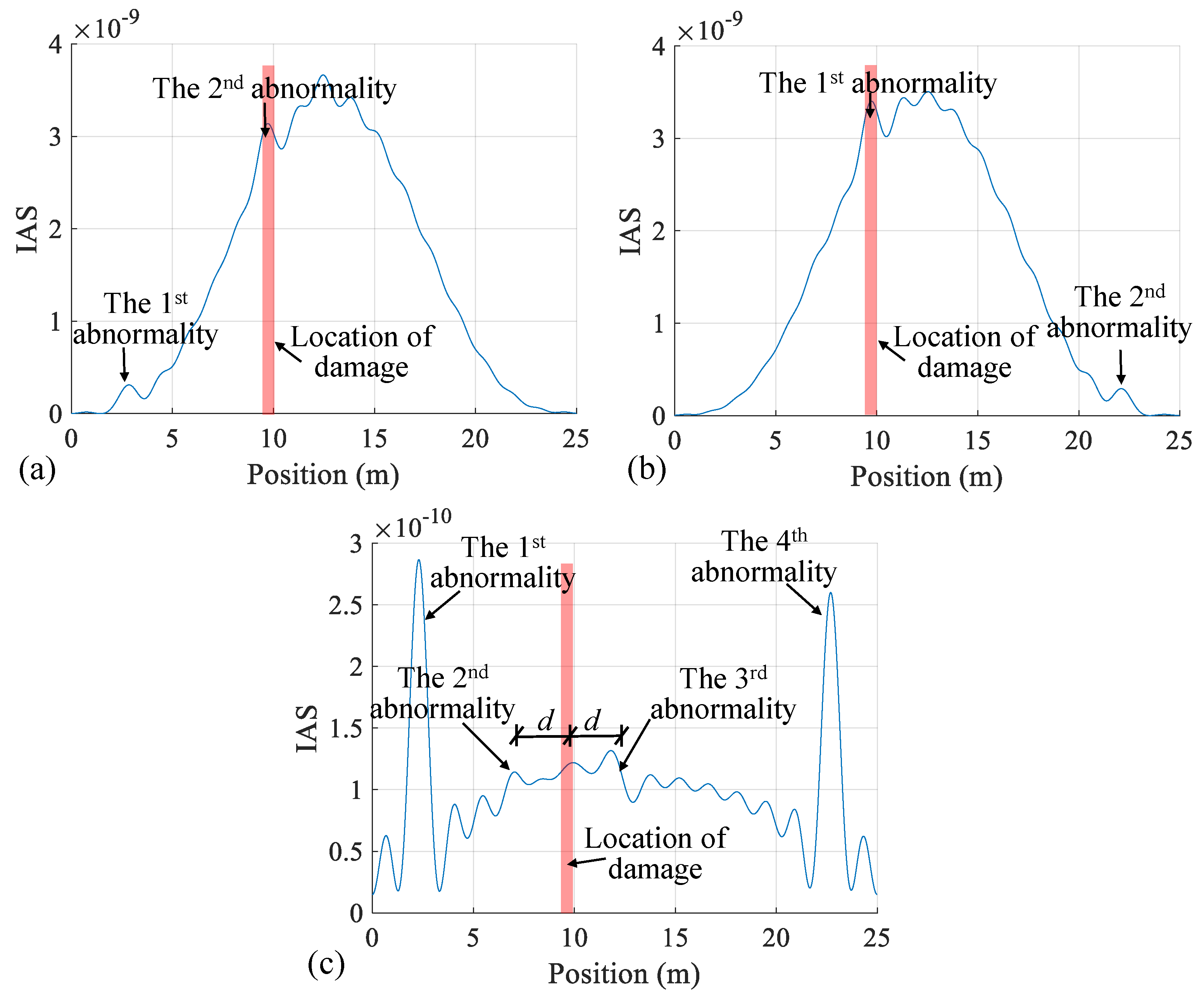
3.3. Numerical Validation of Damage Identification

To validate the proposed IAS index for bridge damage identification, local damage with a 10% reduction in element stiffness was introduced in the 19th beam element, specifically within the range of 9.5 to 10.0 m. In this numerical case, road surface roughness was initially excluded but will be considered in subsequent parametric studies. Figure 5a illustrates the IAS index calculated using the CP acceleration of the vehicle’s front axle. The initial abnormality in the IAS occurs when the front axle approaches 2.6 m, precisely where the rear axle engages with the left boundary of the bridge. The second abnormality in the IAS arises as the front axle approaches the region of 9.5 to 10.0 m, which corresponds to the location of the bridge damage. Similarly, the two anomalies in the IAS of the CP acceleration of the rear axle are observed at approximately 10 m (damage location) and 23 m (where the first axle exits the bridge), as depicted in Figure 5b. Additionally, Figure 5c presents the IAS index of the residual CP acceleration, revealing notable abnormalities near the bridge supports. The IAS of the residual CP acceleration inherits characteristics from the IAS of the CP acceleration of both the front and rear axles. Neglecting the influence of the bridge boundaries, two abnormalities in the IAS near the locations of 7 m and 12 m were roughly observed. The anomaly at 7 m is attributed to the rear axle approaching this point when the front axle is near the location of damage (9.5–10.0 m). Similarly, the front axle approaches 12 m when the rear axle is in proximity to the damaged location. In summary, for a single damage, the location of damage can be determined based on the abnormalities in the IAS for a single-axle test vehicle or the center of two adjacent abnormalities in the IAS for a two-axle test vehicle. Although the authors have marked the localization of the damage in these figures, readers can themselves assess whether these locations precisely correspond to the damage localized based on the changes in the IAS indicators. These findings validate that the proposed IAS effectively detects bridge damage.
Furthermore, road surface roughness is introduced to illustrate the viability of the proposed IAS under such conditions, and the results are presented in Figure 6. In Figure 6a,b, the resulting IAS derived from the CP accelerations of both the front and rear axles fails to identify bridge damage due to the interference of road surface roughness on the CP accelerations. However, as shown in Figure 6c, the IAS derived from the residual CP acceleration exhibits the same capability to identify bridge damage as demonstrated in Figure 5c. Therefore, it is evident that the IAS calculated from the residual CP acceleration demonstrates superiority over the IAS calculated from single axle acceleration in identifying bridge damage in the presence of road surface roughness.

3.4. Influence of Vehicle Speed on Damage Identification

The speed of the test vehicle is a crucial factor influencing the feasibility of the VSM for damage identification [22,23,24,25,26,27,28]. This is because a higher vehicle speed results in fewer vehicle records passing over the bridge, which, in turn, negatively impacts the extraction of the bridge modal information using such limited data. Three sets of vehicle speeds, namely 1 m/s, 2 m/s, and 4 m/s, are compared. For each vehicle speed, three levels of damage—10%, 20%, and 30%—were assigned to the same 19th beam element. Figure 7 presents the influence of vehicle speed on damage identification using the IAS calculated from the residual CP acceleration, where road surface roughness is not involved. It is shown in Figure 7a that all three levels of damage can be identified using the IAS calculated from the residual CP acceleration when the vehicle speed is relatively small, such as 1 m/s. However, when the vehicle speed is increased to 2 m/s, it is observed that the second IAS abnormality at a damage level of 10% becomes insignificant compared to the case with a vehicle speed of 1 m/s. However, when the damage levels are 20% and 30%, the second IAS abnormality becomes visible. Therefore, the damage location can be determined well using the proposed IAS index. When the vehicle speed is 4 m/s, as shown in Figure 7c, the IAS index fails to accurately pinpoint the location of damage across all three damage levels. Therefore, it is advisable to employ low vehicle speeds, such as 1–2 m/s, for enhanced accuracy in using the IAS index for identifying bridge damage.

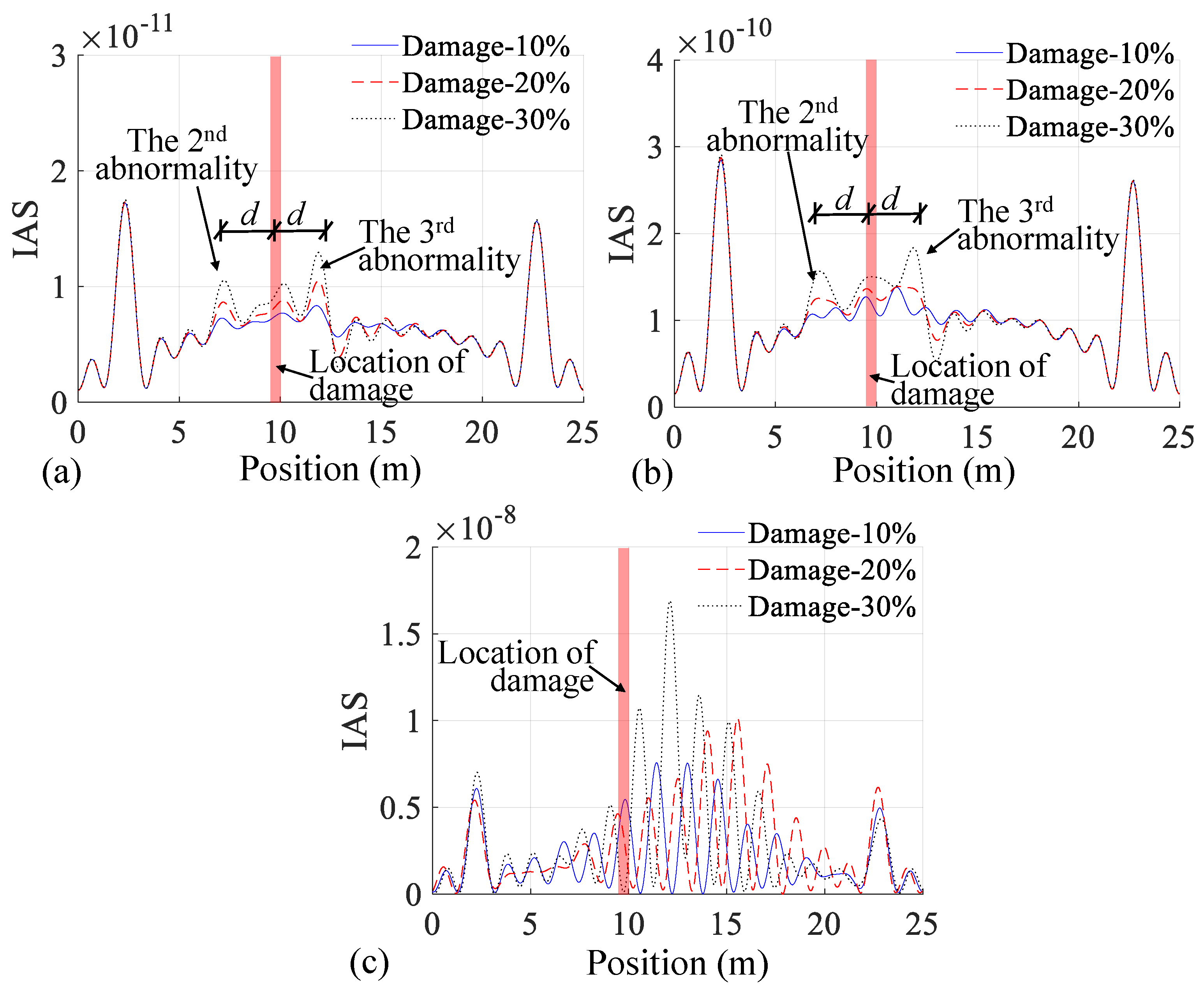
3.5. Influence of Road Roughness on Damage Identification

Road surface roughness is another important factor influencing the feasibility of the VSM for damage identification [22,23,24,25]. Three grades of road surface roughness are analyzed, with Gd(n0) being 0.001 × 10⁻⁶, 2 × 10⁻⁶, and 8 × 10⁻⁶ m3, and representing the ideal laboratory roughness: class A roughness in the ISO standard [22], and class B roughness in the ISO standard [22], respectively. Figure 8 shows the influence of road surface roughness on damage identification using the IAS calculated from the residual CP acceleration. It is shown in Figure 8a that the damage location can be directly identified through the IAS abnormalities when the road is in perfect roughness condition. Additionally, the degrees of damage can be reflected by the degree of abnormality in the IAS index. When the road roughness is set to Gd(n0) = 2 × 10⁻⁶ m3, as shown in Figure 8b, the damage location is almost overwhelmed by the interference of roughness when the damage levels are below 20%. However, the damage location, with a damage level of 30%, can still be identified using the IAS index. The results with Gd(n0) = 8 × 10⁻⁶ m3, as provided in Figure 8c, show similar findings as inferred from those in Figure 8b. These findings reveal that bridge damage can be effectively identified using the IAS index from the residual CP acceleration of a two-axle testing vehicle with the road roughness considered. If the grades of road roughness are much higher, the IAS is feasible for identifying bridge damage only when the damage is significant enough.

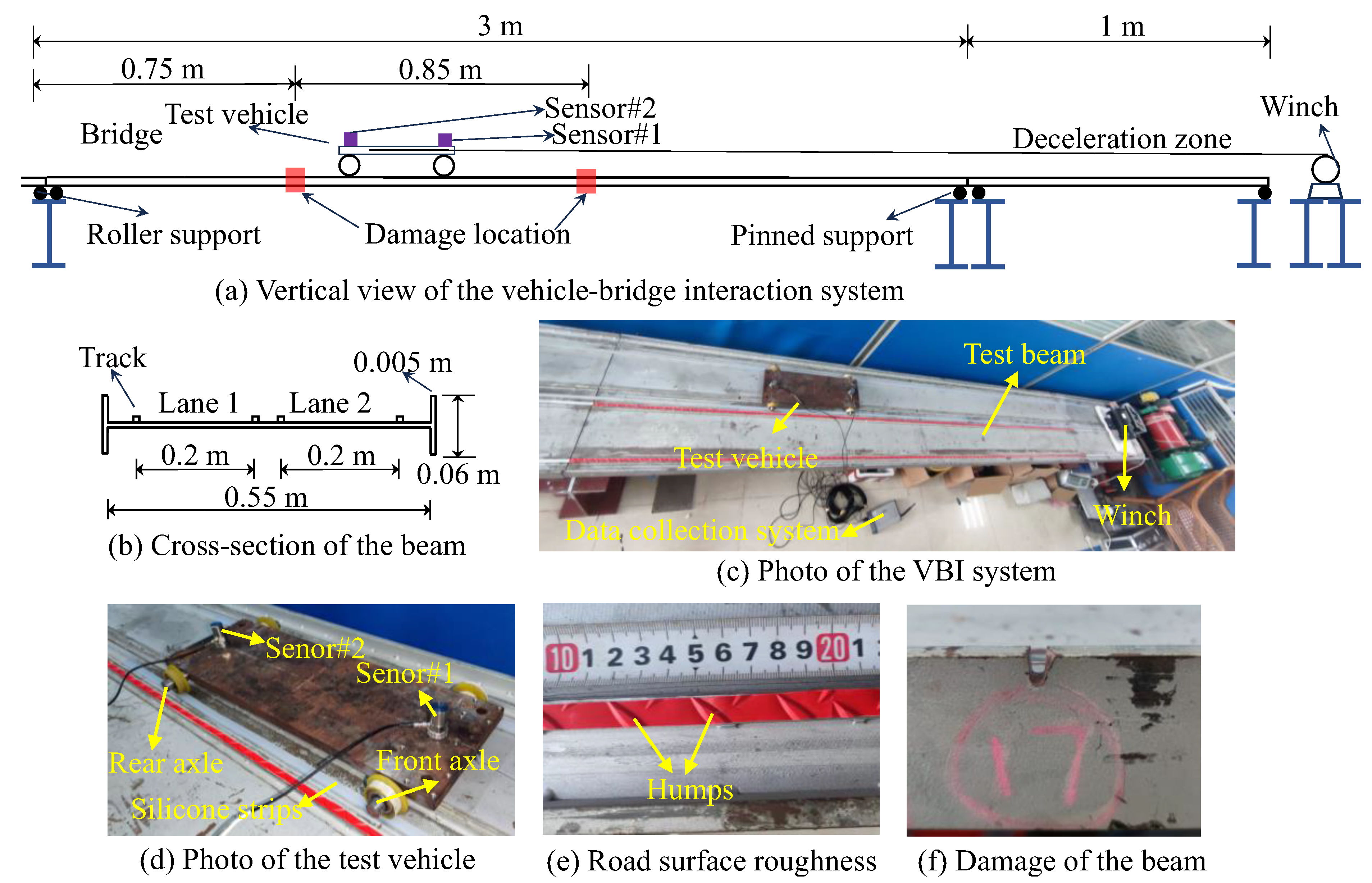
4. Experimental Validations

4.1. The Laboratory VBI System

A laboratory VBI system, as shown in Figure 9, was employed for the experiment to validate the proposed IAS index for indirectly identifying bridge damage. A comprehensive description of the laboratory VBI system is available in a previous study [22]. The first two bridge frequencies were ωb,1 = 7.81 Hz and ωb,2 = 29.29 Hz, which were identified by direct measurements. Notably, the provided bridge frequencies are for the damaged beam. The two-axle test vehicle was composed of two axles, with each axle using a steel bar connecting two polyurethane tires on the left and right, as shown in Figure 9d. A steel plate with a thickness of 12 mm was fixed with the two steel bars. Hence, the test vehicle had relatively large vertical axle stiffnesses. Two accelerometers are mounted on the steel plate directly above the front and rear axles. Since the axle stiffness of the test vehicle is relatively large, the response of the vehicle axle can be treated as proximate to the CP response [25]. The test vehicle was pulled along the tracks across the beam at a constant speed of 0.15 m/s maintained by a winch. The test beam was equipped with two types of tracks: one made of silicone strips used to simulate the idealized perfect road surface roughness, and the other constituted by a non-slip mat on steel rails to simulate a high grade of road surface roughness. Due to the equally spaced arrangement of roughness humps with distances of 16 mm and 32 mm, the vibrational frequencies induced by these humps can be calculated with v/l, i.e., 0.15/0.032 = 4.69 Hz and 0.15/0.016 = 9.38 Hz. The test beam has two damage locations at 0.8 m and 1.7 m of the beam by cutting a 10 mm depth on the edge of the beam, as shown in Figure 9f. The severity of the damage corresponds to a local element stiffness loss of 17.32% with an element length of 10 mm. While this level of damage may be considered relatively severe in real-world conditions, it is quite common in laboratory SHM studies.

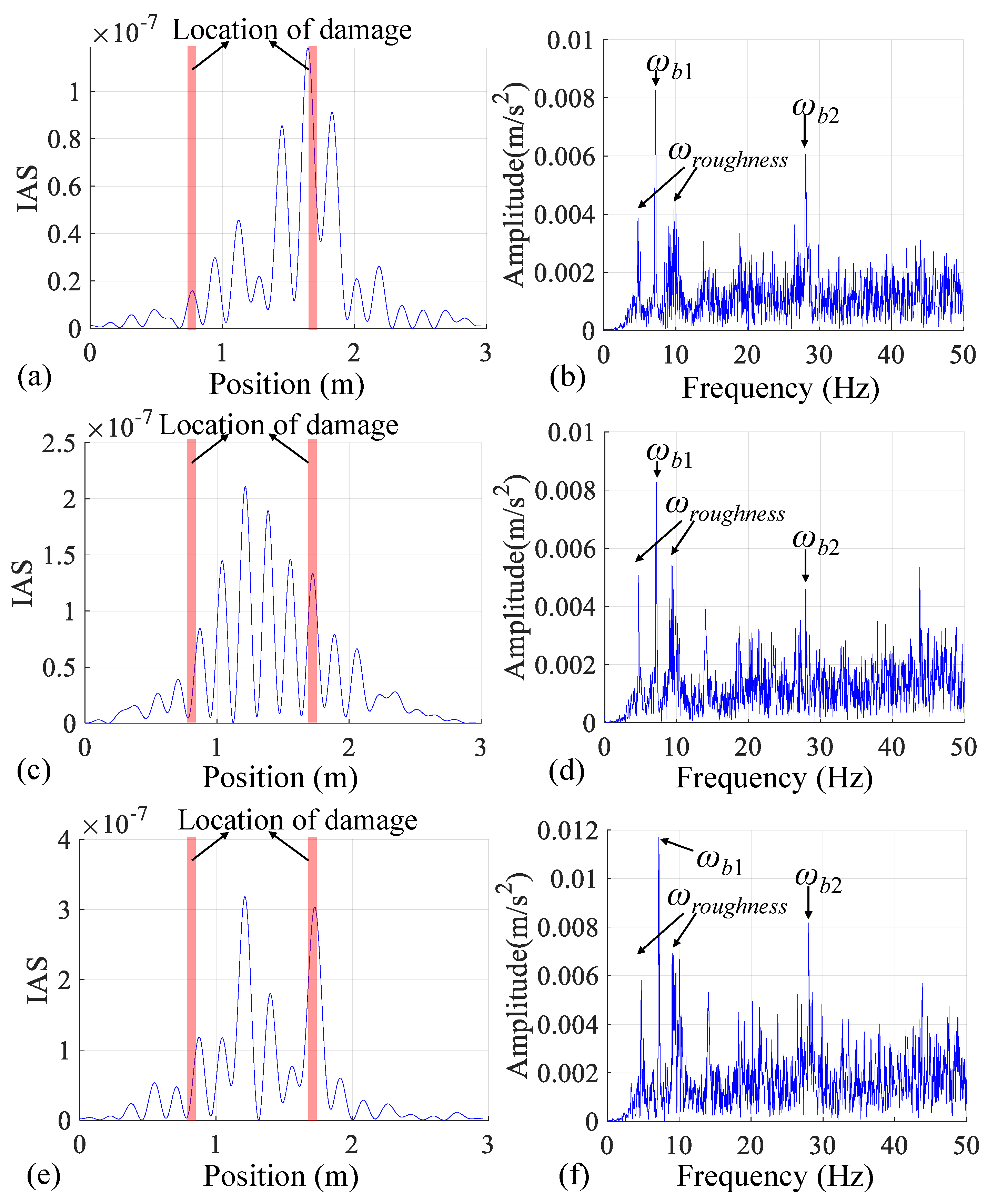
4.2. Damage Detection under the Perfect Road Surface

The perfect road surface was initially considered for the test. The test vehicle was pulled across the track made of silicone strips at a constant speed. The results are presented in Figure 10. In Figure 10a, four obvious abnormalities are observed in the IAS index obtained from the CP acceleration of the front axle, with two abnormalities directly indicating the damage locations of the beam. Similarly, in the IAS index obtained from the CP acceleration of the rear axle (Figure 10c), four abnormalities are detected, and two of them directly indicate the damaged locations of the beam. The IAS index was calculated following the practical procedures shown in Section 2.2. Sensors #1 and #2 measure the vehicle accelerations at the front and rear axles, which can be regarded as y ¨ 1 and y ¨ 2. Additionally, several abnormalities are observed in the IAS index obtained from the residual CP acceleration (Figure 10e), with the two most obvious abnormalities indicating the damage locations in the beam. The presence of other abnormalities that have no relation to the damage is not currently clear and requires further exploration. In terms of the frequency spectra, the first bridge frequency was successfully identified by the CP acceleration at the front axle in Figure 10b, the CP acceleration at the rear axle in Figure 10d, and the residual CP acceleration in Figure 10f. However, the second bridge frequency is not visible from the frequency spectra of these three responses, implying that the residual CP response does not perform better than the CP response in identifying bridge frequencies. In summary, under perfect road surface conditions, the IAS indexes calculated from both CP accelerations and residual CP acceleration were successful in identifying bridge damage. However, the residual CP acceleration does not outperform the CP acceleration, possibly because the test vehicle is too light, and as a result, the bridge vibration is not sufficiently excited.

4.3. Damage Detection under Rough Road Surface

To consider a rough road surface in the experiment, the test vehicle was placed on tracks with non-slip mats, as shown in Figure 9e. The same vehicle speed was maintained, and the results are shown in Figure 11. The findings indicate that the IAS of the front axle CP acceleration identifies the second location of the damage. However, due to the interference of the road surface roughness, the IAS of the front axle CP acceleration includes other irrelevant abnormalities that hinder the identification of the first bridge damage. This phenomenon is particularly evident in the IAS of the rear axle CP acceleration, as shown in Figure 11c. Both locations of damage cannot be identified by the IAS index. In terms of the IAS of the residual CP acceleration, the two damage locations are likely identified by the IAS abnormalities. However, other obvious IAS abnormalities were also presented, which have no relation to the bridge damage. In terms of the frequency spectra, the first and second bridge frequencies were all successfully identified by the CP acceleration at the front axle in Figure 11b, CP acceleration at the rear axle in Figure 11d, and residual CP acceleration in Figure 11f. Additionally, the influence of the roughness also includes introducing the roughness frequency ωroughness in the spectrum of the CP responses. These interferences are inherited in the residual response, which may be another influencing factor in the recognition of damage. The reason why the second bridge frequency can be identified is that the bridge vibration is significant under the excitation of rough road roughness, making the bridge frequency easier to identify; however, such effects are not favorable for the identification of bridge damage. In conclusion, the experiments only demonstrate the weak possibility of using the IAS extracted from residual CP response for identifying bridge damage. However, further experiments should be performed to fully examine the capacity of the IAS for bridge damage identification in practical applications.

5. Conclusions

This study focuses on identifying bridge damage using the response of a two-axle passing vehicle. The closed solution of residual CP acceleration is derived for a two-axle vehicle interacting with a simply supported beam. The IAS index is then constructed from the driving frequency of the residual CP acceleration to identify bridge damage. Numerical investigations using finite element simulation, as well as experimental validations through laboratory VBI tests, were conducted to verify the proposed damage detection approach. The main findings are as follows:
(1)
The IAS index of the residual CP acceleration can be constructed by applying a multi-peak idealized filter and the Hilbert transform to the driving frequency spectra. This index is theoretically sensitive to the bridge modal shape and can be used to identify bridge damage. Theoretically, it eliminates the influence of vehicle self-vibrations and road roughness when the vehicle–bridge coupling effect can be ignored;
(2)
Numerical investigations verify the accuracy of the theoretical derivations. The bridge damage can be determined by observing IAS abnormalities, which are baseline-free. The IAS of the residual CP acceleration can identify a 10% stiffness loss in a beam element under low road surface roughness and a 30% stiffness loss under high road surface roughness. A favorable vehicle speed of no greater than 2 m/s yields good damage identification results;
(3)
Laboratory tests show that it is possible to roughly identify bridge damage using the IAS extracted from residual CP acceleration under perfect road surfaces. The results of the IAS from residual CP acceleration show the same ability to locate damage as those of the IAS from CP accelerations at the front or rear axle. However, some irrelevant IAS abnormalities were observed, which have no relation to the bridge damage;
(4)
Regarding rough road surfaces in the experimental setup, while both IAS indicators derived from residual CP acceleration and axle CP acceleration successfully identify multiple bridge frequencies, it is likely that they both fall short in detecting damage. Hence, further experiments should be performed to fully examine the capacity of the IAS for bridge damage identification in practical applications.
This study shows some theoretical and experimental attempts at using the IAS from residual CP responses for bridge damage identification. The feasibility of residual CP responses is not examined in the literature, and this gap was filled by this study to some extent. Based on the findings of this study, it is possible to employ an ordinary two-axle commercial vehicle for the indirect detection of bridge damage, thereby enabling the rapid estimation of structural health for a large group of bridges using only these vehicles. However, more experiments should be conducted to further validate the theoretical superiority of the residual CP response for the indirect identification of bridge modal properties. Furthermore, exploring the feasibility of the IAS index for detecting damage in beams with other boundary conditions represents a significant area for future research. Additionally, considering the incorporation of machine learning algorithms for predicting bridge damage, particularly with an expanded dataset of the IAS, represents a meaningful future endeavor. Exploring the potential of the proposed method to identify multiple damage regions through numerical investigations would also be meaningful follow-up work.

Author Contributions

Conceptualization, J.Z.; Methodology, Z.Z.; Software, J.Z.; Validation, S.L. and Z.Z.; Investigation, S.L.; Data curation, S.L. and Y.Z.; Writing—original draft, S.L. and Z.Z.; Writing—review & editing, J.D. and J.Z.; Supervision, J.D. and J.Z.; Project administration, Z.S.; Funding acquisition, J.Z. All authors have read and agreed to the published version of the manuscript.

Funding

This research was supported by the Fundamental Research Program of Guangzhou Municipal College Joint Fund (SL2023A03J00897) and the College Student Innovation and Entrepreneurship Program of Guangzhou University (S202311078055 and S202311078017).

Data Availability Statement

Data are available based on reasonable request from the corresponding author.

Conflicts of Interest

The authors declare that they have no known competing financial interests or personal relationships that could have appeared to influence the work reported in this paper.

References

  1. Sun, L.; Shang, Z.; Xia, Y.; Bhowmick, S.; Nagarajaiah, S. Review of bridge structural health monitoring aided by big data and artificial intelligence: From condition assessment to damage detection. J. Struct. Eng. 2020, 146, 04020073. [Google Scholar] [CrossRef]
  2. An, Y.; Chatzi, E.; Sim, S.H.; Laflamme, S.; Blachowski, B.; Ou, J. Recent progress and future trends on damage identification methods for bridge structures. Struct. Control Health Monit. 2019, 26, e2416. [Google Scholar] [CrossRef]
  3. Brownjohn, J.M.; De Stefano, A.; Xu, Y.L.; Wenzel, H.; Aktan, A.E. Vibration-based monitoring of civil infrastructure: Challenges and successes. J. Civ. Struct. Health Monit. 2011, 1, 79–95. [Google Scholar] [CrossRef]
  4. Hou, R.; Xia, Y. Review on the new development of vibration-based damage identification for civil engineering structures: 2010–2019. J. Sound Vib. 2021, 491, 115741. [Google Scholar] [CrossRef]
  5. Wang, Z.L.; Yang, J.P.; Shi, K.; Xu, H.; Qiu, F.Q.; Yang, Y.B. Recent advances in researches on vehicle scanning method for bridges. Int. J. Struct. Stab. Dyn. 2022, 22, 2230005. [Google Scholar] [CrossRef]
  6. Shokravi, H.; Shokravi, H.; Bakhary, N.; Heidarrezaei, M.; Rahimian Koloor, S.S.; Petrů, M. Vehicle-assisted techniques for health monitoring of bridges. Sensors 2020, 20, 3460. [Google Scholar] [CrossRef]
  7. Malekjafarian, A.; Corbally, R.; Gong, W. A review of mobile sensing of bridges using moving vehicles: Progress to date, challenges and future trends. Structures 2022, 44, 1466–1489. [Google Scholar] [CrossRef]
  8. Yang, Y.B.; Lin, C.W.; Yau, J.D. Extracting bridge frequencies from the dynamic response of a passing vehicle. J. Sound Vib. 2004, 272, 471–493. [Google Scholar] [CrossRef]
  9. Nagayama, T.; Reksowardojo, A.P.; Su, D.; Mizutani, T. Bridge natural frequency estimation by extracting the common vibration component from the responses of two vehicles. Eng. Struct. 2017, 150, 821–829. [Google Scholar] [CrossRef]
  10. Xu, H.; Huang, C.C.; Wang, Z.L.; Shi, K.; Wu, Y.T.; Yang, Y.B. Damped test vehicle for scanning bridge frequencies: Theory, simulation and experiment. J. Sound Vib. 2021, 506, 116155. [Google Scholar] [CrossRef]
  11. Yang, Y.; Lu, H.; Tan, X.; Wang, R.; Zhang, Y. Mode shape identification and damage detection of bridge by movable sensory system. IEEE T. Intell. Transp. 2022, 24, 1299–1313. [Google Scholar] [CrossRef]
  12. Li, J.; Zhu, X.; Guo, J. Bridge modal identification based on successive variational mode decomposition using a moving test vehicle. Adv. Struct. Eng. 2022, 25, 2284–2300. [Google Scholar] [CrossRef]
  13. Yin, X.; Yang, Y.; Huang, Z. Bridge frequency extraction method based on contact point response of two-axle vehicle. Structures 2023, 57, 105176. [Google Scholar] [CrossRef]
  14. Hashlamon, I.; Nikbakht, E. Theoretical and numerical investigation of bridge frequency identification employing an instrumented vehicle in stationary and moving states. Structures 2023, 51, 1684–1693. [Google Scholar] [CrossRef]
  15. Zhan, Y.; Au, F.T.; Zhang, J. Bridge identification and damage detection using contact point response difference of moving vehicle. Struct. Control Health Monit. 2021, 28, e2837. [Google Scholar] [CrossRef]
  16. Yang, D.S.; Wang, C.M. Bridge damage detection using reconstructed mode shape by improved vehicle scanning method. Eng. Struct. 2022, 263, 114373. [Google Scholar] [CrossRef]
  17. He, Y.; Yang, J.P.; Yan, Z. Enhanced identification of bridge modal parameters using contact residuals from three-connected vehicles: Theoretical study. Structures 2023, 54, 1320–1335. [Google Scholar] [CrossRef]
  18. Liu, Y.; Zhan, J.; Wang, Y.; Wang, C.; Zhang, F. An effective procedure for extracting mode shapes of simply-supported bridges using virtual contact-point responses of two-axle vehicles. Structures 2023, 48, 2082–2097. [Google Scholar] [CrossRef]
  19. Hajializadeh, D. Deep learning-based indirect bridge damage identification system. Struct. Control Health Monit. 2023, 22, 897–912. [Google Scholar] [CrossRef]
  20. Hurtado, A.C.; Kaur, K.; Alamdari, M.M.; Atroshchenko, E.; Chang, K.C.; Kim, C.W. Unsupervised learning-based framework for indirect structural health monitoring using adversarial autoencoder. J. Sound Vib. 2023, 550, 117598. [Google Scholar] [CrossRef]
  21. Li, Z.; Lin, W.; Zhang, Y. Real-time drive-by bridge damage detection using deep auto-encoder. Structures 2023, 47, 1167–1181. [Google Scholar] [CrossRef]
  22. Zhou, J.; Lu, Z.; Zhou, Z.; Pan, C.; Cao, S.; Cheng, J.; Zhang, J. Extraction of bridge mode shapes from the response of a two-axle passing vehicle using a two-peak spectrum idealized filter approach. Mech. Syst. Signal Pr. 2023, 190, 110122. [Google Scholar] [CrossRef]
  23. Xu, H.; Yang, M.; Yang, J.P.; Wang, Z.L.; Shi, K.; Yang, Y.B. Vehicle scanning method for bridges enhanced by dual amplifiers. Struct. Control Health Monit. 2023, 2023, 6906855. [Google Scholar] [CrossRef]
  24. Yang, Y.B.; Li, Z.; Wang, Z.L.; Shi, K.; Xu, H.; Qiu, F.Q.; Zhu, J.F. A novel frequency-free movable test vehicle for retrieving modal parameters of bridges: Theory and experiment. Mech. Syst. Signal Pr. 2022, 170, 108854. [Google Scholar] [CrossRef]
  25. Zhou, Z.; Zhou, J.; Deng, J.; Wang, X.; Liu, H. Identification of multiple bridge frequencies using a movable test vehicle by approximating axle responses to contact-point responses: Theory and experiment. J. Civ. Struct. Health Monit. 2024. under review. [Google Scholar]
  26. Zhang, B.; Qian, Y.; Wu, Y.; Yang, Y.B. An effective means for damage detection of bridges using the contact-point response of a moving test vehicle. J. Sound Vib. 2018, 419, 158–172. [Google Scholar] [CrossRef]
  27. Feng, K.; Casero, M.; González, A. Characterization of the road profile and the rotational stiffness of supports in a bridge based on axle accelerations of a crossing vehicle. Comput. Aided Civ. Inf. 2023, 38, 12974. [Google Scholar] [CrossRef]
  28. Yang, Y.B.; Xu, H.; Wang, Z.L.; Shi, K. Using vehicle–bridge contact spectra and residue to scan bridge’s modal properties with vehicle frequencies and road roughness eliminated. Struct. Control Health Monit. 2022, 29, e2968. [Google Scholar] [CrossRef]
  29. Hashlamon, I.; Nikbakht, E. The use of a movable vehicle in a stationary condition for indirect bridge damage detection using baseline-free methodology. Appl. Sci. 2022, 12, 11625. [Google Scholar] [CrossRef]
  30. Ma, X.; Roshan, M.; Kiani, K.; Nikkhoo, A. Dynamic response of an elastic tube-like nanostructure embedded in a vibrating medium and under the action of moving nano-objects. Symmetry 2023, 15, 1827. [Google Scholar] [CrossRef]
  31. Yu, G.; Kiani, K.; Roshan, M. Dynamic analysis of multiple-nanobeam-systems acted upon by multiple moving nanoparticles accounting for nonlocality, lag, and lateral inertia. Appl. Math. Model. 2022, 108, 326–354. [Google Scholar] [CrossRef]
  32. Dimitrovová, Z. Dynamic interaction and instability of two moving proximate masses on a beam on a Pasternak viscoelastic foundation. Appl. Math. Model. 2021, 100, 192–217. [Google Scholar] [CrossRef]
  33. Zhou, J.; Zhou, Z.; Jin, Z.; Liu, S.; Lu, Z. Comparative study of damage modeling techniques for beam-like structures and their application in vehicle-bridge-interaction-based structural health monitoring. J. Vib. Control 2023, 10775463231209357. [Google Scholar] [CrossRef]
  34. Xiao, J.; Huang, L.; He, Z.; Qu, W.; Li, L.; Jiang, H.; Zhong, Z.; Long, X. Probabilistic models applied to concrete corrosion depth prediction under sulfuric acid environment. Measurement 2024, 234, 114807. [Google Scholar] [CrossRef]
Figure 1. Schematic representation of a two-axle vehicle interacting with a simply supported beam.
Buildings 14 01428 g001
Figure 2. Finite element simulation of a symmetric two-axle vehicle interacting with a simply supported beam.
Buildings 14 01428 g002
Figure 3. Comparison of the CP response at the front axle of a two-axle vehicle calculated by different methods: (a) CP displacement; (b) Spectrum of CP acceleration.
Buildings 14 01428 g003
Figure 4. Residual CP response of the two-axle test vehicle back-calculated from the vehicle responses: (a) Residual CP acceleration; (b) Spectrum of residual CP acceleration.
Buildings 14 01428 g004
Figure 5. Comparison of damage identification results using the IAS calculated by various CP responses without road surface roughness: (a) CP acceleration of the front axle; (b) CP acceleration of the rear axle; (c) residual CP acceleration.
Buildings 14 01428 g005
Figure 6. Comparison of damage identification results using the IAS calculated by various CP responses with road surface roughness of Gd(n0) = 0.001 × 10⁻⁶m3: (a) CP acceleration of the front axle; (b) CP acceleration of the rear axle; (c) residual CP acceleration.
Buildings 14 01428 g006
Figure 7. Influence of vehicle speed on damage identification using the IAS calculated from the residual CP acceleration: (a) 1 m/s, (b) 2 m/s, and (c) 4 m/s.
Buildings 14 01428 g007
Figure 8. Influence of road surface roughness on damage identification using the IAS calculated from the residual CP acceleration: (a) Gd(n0) = 0.001 × 10⁻⁶ m3, (b) Gd(n0) = 2 × 10⁻⁶ m3, and (c) Gd(n0) = 8 × 10⁻⁶ m3.
Buildings 14 01428 g008
Figure 9. Schematic diagram and photos of the laboratory VBI system.
Buildings 14 01428 g009
Figure 10. Results under the perfect road surface: (a) IAS of the CP acceleration at the front axle; (b) frequency spectra of the CP acceleration at the front axle; (c) IAS of the CP acceleration at the rear axle; (d) frequency spectra of the CP acceleration at the rear axle; (e) IAS of the residual CP acceleration; (f) frequency spectra of the residual CP acceleration.
Buildings 14 01428 g010
Figure 11. Results under the rough road surface: (a) IAS of the CP acceleration at the front axle; (b) frequency spectra of the CP acceleration at the front axle; (c) IAS of the CP acceleration at the rear axle; (d) frequency spectra of the CP acceleration at the rear axle; (e) IAS of the residual CP acceleration; (f) frequency spectra of the residual CP acceleration.
Buildings 14 01428 g011
Table 1. Parameter values of the test vehicle and bridge.
ItemParametersSymbolUnitValue
VehicleMass of vehicle Mvkg1000
Mass moment of vehicle Jvkg·m2900
Stiffness of front axlek1N/m3.5 × 105
Stiffness of rear axlek2N/m4 × 105
Distance from the front axlel1m1.35
Distance from the rear axlel2m1.25
Velocityvm/s2
Bridge LengthLm25
Young’s modulusEMPa2.75 × 104
Moment of inertiaIm40.20
Mass per unit lengthmkg/m2400
Disclaimer/Publisher’s Note: The statements, opinions and data contained in all publications are solely those of the individual author(s) and contributor(s) and not of MDPI and/or the editor(s). MDPI and/or the editor(s) disclaim responsibility for any injury to people or property resulting from any ideas, methods, instructions or products referred to in the content.

