
Design and Validation of a Stratified Shear Model Box for Seismic Response of a Sand-Blowing Reclamation Site
1
The Campus of Xixiangtang, Nanning College for Vocational Technology, Nanning 530008, China
2
Nnaning Newhope Real Estate Co., Ltd., Nanning 530009, China
3
School of Civil Engineering and Architecture, Guangxi Minzu University, Nanning 530008, China
4
Guangxi Xinfazhan Communication Group Co., Ltd., Nanning 530022, China
5
School of Public Policy and Management, Guangxi University, Nanning 530004, China
6
School of Civil Engineering and Architecture, Guangxi Vocational & Technical Institute of Industry, Nanning 530003, China
*
Author to whom correspondence should be addressed.
Buildings 2024, 14(5), 1405; https://doi.org/10.3390/buildings14051405
Submission received: 10 April 2024
/
Revised: 1 May 2024
/
Accepted: 9 May 2024
/
Published: 14 May 2024
(This article belongs to the Special Issue Construction in Urban Underground Space)
Abstract
:The global increase in building collapses and damage on soft-soil sites due to distant significant earthquakes poses similar challenges for sand-blowing reclamation (SBR) sites on soft-soil layers. This study was initiated to capture the vibration characteristics of the SBR sites and to provide fresh insights into their seismic responses. Initially, considering the heterogeneity and layered structure of soil at SBR sites, we developed a novel stratified shearing model box. This model box enables the simulation of the complex characteristics of soil layers at SBR sites under laboratory conditions, representing a significant innovation in this field. Subsequently, an innovative jack loading system was developed to apply active vertical pressure on the soil layer model, accelerating soil consolidation. Furthermore, a new data collection and analysis system was devised to monitor and record acceleration, pore water pressure, and displacement in real time during the experiments. To verify the model box’s accuracy and innovation, and to examine the seismic response of SBR sites under varying consolidation pressures, four vibration tests were conducted across different pressure gradients to analyze the model’s predominant period evolution due to consolidation pressures. The experimental results demonstrate that the model box accurately simulates the propagation of one-dimensional shear waves in soil layers under various consolidation pressures, with notable repeatability and reliability. Our experiments demonstrated that increasing consolidation pressure results in higher shear wave speeds in both sand and soft-soil layers, and shifts the site’s predominant period towards shorter durations. Concurrently, we established the relationship between the site’s predominant period and the input waves. This study opens new paths for further research into the dynamic response properties of SBR sites under diverse conditions through shaking-table tests.
1. Introduction
In recent years, powerful distant earthquakes have triggered sporadic engineering seismic damage all around the world; buildings have also been severely destroyed by distant earthquake waves. The extensive damage to buildings during the Kahramanmaraş earthquake in Turkey (see Figure 1) was due to the low strength of adobe material, the usage of heavy earthen roofs, the failure to comply with earthquake-resistant building design principles, and the insufficient support provided to load-bearing walls [1]. An earthquake measuring 6.3 on the Richter scale struck the western province of Herat in Afghanistan (see Figure 2), resulting in significant casualties and losses. The disaster claimed the lives of at least 1482 people and injured over 2000, including women and children [2]. The 2023 Mw 6.8 earthquake in Al Haouz, Morocco, underscores the limited understanding of the seismogenic processes associated with mountain building in this expansive plate boundary region [3].
The seismic damage inflicted on soft-soil sites is extremely notable. For instance, numerous buildings on soft-soil foundations collapsed during a magnitude 8.0 earthquake 300 km from Mexico City in 1985 [4,5]. The 1989 Loma Prieta earthquake, with a magnitude of 7.1 on the Richter scale, destroyed bridges and overpasses constructed on soft soils in the Bay area [6,7,8]. It is widely accepted that the primary cause of building destruction is the propagation of earthquake waves in deep soft soils, which increases their long-period component. This causes the fundamental period of the buildings to coincide with the predominant period of the site, leading to the resonance damage [9,10,11].
In the context of the seismic damage mentioned above, SBR sites of thick soft soil with layered structures are usually located in coastal areas with relatively high seismicity and have thick–very thick layers of soft soils, like those in the areas of seismic damage described above [12,13,14]. This human-made rock and soil structure located on coastal sediments consists of thick layers of marine soft soil and sandy soil. Due to the relatively short formation period of the soil layer, its consolidation is in a constant state of initial change. The features of the sea accumulation layer and the reclamation layer continue to evolve under the continuing influence of the construction of the reclaimed land. Some studies have indicated that the predominant period of the site may vary over time [15,16].
To gain a deeper understanding of the behavior of SBR sites under varying dynamic stimuli, laboratory studies—by using models based on these sites, under controlled dynamic test conditions—can offer valuable insights [17,18,19,20,21,22,23]; here, shaking-table tests are widely used. Researchers typically utilize three types of model boxes in their shaking-table test studies, i.e., rigid, flexible cylindrical, and stratified [24,25,26]. The stratified shearing model box performs well in eliminating boundary effects and accommodating the horizontal layered deformation of the soil. This model box is superior to the other two model boxes in simulating soil shear deformation. As a result, the unique features of the stratified shearing model boxes have promoted their applications in shaking-table tests on geotechnical structures in recent years [24,27,28,29]. These available studies lead to the model box developed in our study, which also incorporates the same stratified structure and continues the use of this efficient design.
The design of a novel model box characterized by flexible and frictional boundaries requires specific critical conditions to be satisfied. These are essential to accurately simulate the infinite lateral extension of the soil present in the prototype and to meet the experimental requirements. The design of a model box for simulating soil dynamics under seismic conditions presents significant challenges in minimizing the interaction between soil and sidewalls to reduce boundary effects. The solution to the second challenge involves accurate simulation of the preload to accelerate the consolidation of the soil layer. In view of the above issues, a large, stratified shearing box and a loading system were developed in this study, and a series of shaking-table tests were conducted to investigate the influence of soil consolidation on the predominant period of the site. A total of four vibration tests at varying pressure gradients were performed to analyze the influence of consolidation state on evolution of the predominant period of the model.
2. Devices and Materials Utilized for the Shaking-Table Test
2.1. Shaking Table
Shaking-table tests were conducted at the Key Laboratory of Disaster Prevention and Structural Safety of the Chinese Ministry of Education at Guangxi University, China. The tests were performed on a computer-controlled, servo-hydraulic, single-degree-of-freedom (horizontal) shaking table (see Figure 3). The shaking table has a 3 m × 3 m loading platform that can provide an effective load of 10 tons, which can meet a variety of experimental needs. A digitally controlled servo-hydraulic actuator provides the shaking action to ensure precise and controllable vibration. The dedicated control room is equipped with a comprehensive control system (including a host) that facilitates a series of tests under constant amplitude and pseudo-random conditions. The shaking table operates at an acceleration between 0.05 g and 1.3 g and a frequency between 0.4 Hz and 40 Hz. These parameters can be adjusted according to experimental requirements. The shaking table has a maximum allowable speed of 0.5 m/s, allowing it to conduct high-intensity vibration tests within a safe speed range.
2.2. Model Box Design
The model box must fulfill several critical criteria to ensure the integrity and success of the experiments.
- Durability: it should be robust enough to prevent instability or damage during vibrations.
- Size considerations: it must be properly sized to ensure that the total weight remains within the maximum capacity of the shaking table.
- Resonance avoidance: resonance with the self-vibration frequencies of the model soil should be avoided.
- Boundary effect reduction: efforts must be made to minimize boundary effects.
The design of the model box significantly affects the accuracy of the experimental results, emphasizing the need for precise dimensions of the model box.
For the model box frame, our initial material choices included pure iron, aluminum, steel, copper, plastic, and PVC. After reviewing relevant materials, we determined that steel not only meets the structural requirements of the model box but also offers the best balance of cost-effectiveness and durability. To avoid resonance due to matching natural frequencies between the model box and the model, we devised a solution that involves welding bow-shaped steel plates to the sides of the model box. This adjustment alters its natural frequency and prevents resonance. To replicate the undrained consolidation conditions of soil layers during earthquakes, a seepage barrier made of geotextile, a rubber membrane, and a plastic film was installed inside the model box. This barrier effectively prevents the leakage of silt and water. These modifications and their implications will be explored in greater detail in subsequent sections.
The dimensions of the model box are limited by the size and specifications of the shaking table. Considering the distribution of screw holes and the operational weight capacity of the shaking table, the model box in this study was designed to be 2.0 m in length, 1.0 m in width, and 1.6 m in height. Due to the corrosive nature of marine soft soil, stainless-steel square tubes were chosen as the framework material for the model box.
For clarity of description, the directions along the short and long axes of the model box are denoted as the X and Y directions, respectively, while the vertical direction is denoted as the Z direction. It was assumed that the average mass of the soil was 1800 kg/m3 and the height of the model was 1.5 m. A vertical load of 30 kPa was applied to the top of the model. The lateral pressure coefficient K0 was determined to be 0.45, as illustrated in Figure 4a. The lateral pressure of the soil was estimated as follows:
where σx and σy represent the lateral pressures in the X and Y directions, respectively; ρ is the soil density; and h is the height of the soil layer.
The calculated values of σx and σy by Equation (1) were both 25.4 kPa. Force analysis of the model revealed that bottom frame of the model box was particularly prone to bending and shearing damage. This bottom frame was modeled as a simply supported beam for bending analysis, as illustrated in Figure 4b. The maximum tensile and shear stresses of the model box frame with a thickness ranging from 0.9 to 3 mm are detailed in Table 1. Stainless-steel square tubes with a thickness between 0.9 and 3 mm and a yield strength of 210 MPa [30] adequately met the strength requirement. The 1 mm thick stainless-steel square tubes were adopted for the fabrication of the model box, which allowed for the goals of robust structural integrity and minimizing the self-weight of the box.
A horizontal vibration motion of the site model is mandated to conform to the deformation criteria associated with a one-dimensional shear beam [31,32]. Therefore, the intrinsic frequency of the designed model box must be significantly different from that of the site model to prevent resonance [33]. This study introduced a bow-shaped steel plate placed on the sidewalls of the model for connecting the layered frames, as depicted in Figure 5.
The intrinsic frequency of the model box was adjusted by varying the thickness of the bow-shaped steel plates. Equations for estimating the intrinsic frequencies of the site model and the model box were provided, and they were influenced by bow-shaped steel plates with varying thicknesses. The intrinsic frequency of the model foundation is calculated with Equation (2).
where denotes the shear wave velocity, Gmax is the maximum shear modulus of the soil, H is the height of the soil layer, and ρ is the soil density. Generally, empirical methods are employed to determine the maximum shear modulus (Gmax) of the soil. The empirical formula for determining the Gmax of the soil proposed by [34] is as follows:
where σ0 is the average effective consolidation stress, and e is the void ratio. The K0 (see Formula (1)) was set to 0.45 [35]. The average effective stress and the shear modulus Gmax at a depth of 0.75 m in the middle section of the model were measured to be 8.4 kN/m2 and 18.2 MPa, respectively. Substituting the shear modulus Gmax into Formula (2) yielded an estimated intrinsic frequency of approximately 16 Hz for the model.
The modal analysis of the model box was conducted using ANSYS software (version 19.2), where the shell 63 elements were adopted to simulate the box frame and bow-shaped stiffeners (see Figure 6). During the modal analysis, the model box was allowed to displace along the vibration direction, but its displacements in other directions were restricted. The 304 stainless steels at room temperature (20 °C) have an elastic modulus of 195 × 109 Pa, a density of 7900 kg/m3, and a Poisson’s ratio of 0.247. The bottom of the model was fixed. Table 2 lists the first-, second-, and third-order intrinsic frequencies along the excitation direction of the model box containing bow-shaped stiffeners with thicknesses of 0.8 mm, 1.0 mm, 1.2 mm, and 1.5 mm, as determined by the modal analysis.
The results in Table 2 indicated that the use of thinner, bow-shaped steel plates led to a significant deviation from the intrinsic frequency of the model soil, thus producing more favorable outcomes in experiments. Therefore, a bow-shaped steel plate with a thickness of 0.7 mm was chosen in this study.
According to the above calculation results, the stratified shearing model box presented in this paper consists of 16 independently stacked hollow square tube frames. Each frame layer is 2090 mm long, 1000 mm wide, and 10 mm in height, and it is made of stainless-steel rectangular hollow square tubes. Each square tube has a cross-section of 95 mm × 45 mm and a thickness of 1 mm. Stainless-steel U-shaped channel guide rails are welded to the upper surface of each middle frame layers except for the first and topmost layers. Meanwhile, the lower surface is affixed with 6 cm high steel pulleys. The spacing between each frame layer is 10 mm, which facilitates the layers to slide over each other when stacked. Stainless-steel bow-shaped stiffeners are attached to the outer surface of the X-direction frame of the model box to fix the two adjacent layers of the frame together. The bow-shaped stiffeners provide dual functions of regulating intrinsic frequency and restricting lateral deformation of the model box. This ensures that each frame layer experiences unidirectional vibration along the direction of excitation during the vibration process. To prevent sludge and water leakage through the frame gaps inside the model, a sealing layer was incorporated into the shearing box in this study. This layer was composed of geotextiles, rubber membranes, and plastic films, as presented in Figure 7.
2.3. Loading Device
As illustrated in Figure 8 the loading device on the shaking table is an integrated system consisting of four essential components, i.e., a transmission screw, an upper steel beam, a jack, and a steel plate. The jack serves as the main pressure source and works conjunction with the upper steel beam and the transmission screw to distribute the load uniformly into the soil layer through the steel plate, thus maintaining a consistent pressure for soil consolidation. The upper steel beam consists of seven 100 mm × 100 mm × 8 mm square steel tubes and two 3000 mm long parallel 18# I-beams. The square steel tubes have reserved bolt holes at both ends to connect the screws (see Figure 9). The screws are 2300 mm long and are connected to the base and steel frame at both ends to transfer the load. The comprehensive jack loading system consists of an oil source, two jacks, a pressure sensor, and a CNC operator console. This setup capable of monitoring the internal oil pressure in the jack can automatically pressurize or cease operation in case the oil pressure deviates from the preset value. The steel plate with dimensions of 1970 mm × 790 mm × 10 mm plays an indispensable role in transferring the reaction force from the device to the model soil.
2.4. Sensors
An integrated assembly of ten accelerometers, eight pore water pressure transducers, and two linear variable differential transformers was positioned in the fill site model to ensure accurate and thorough data collection (see Figure 10). The acceleration sensors and pore water manometers were arranged in the sand and soft-soil layers according to Figure 10 and the laser displacement sensors were installed on the top surface of the model soil layer. The accelerometer with the analog voltage output variety offers an impressive acceleration range of 1 g. To ensure precise measurement of the top settlement, two non-contact linear variable differential transformers were strategically installed on the upper surface of the model soil. These sensors, with a sensing range of 30 to 300 mm and a response time of 20 ms, captured timely and accurate soil displacement data.
3. Model Construction
3.1. Test Soil
To enhance the validity of experimental results, a model that simulates the typical environmental conditions of SBR sites was developed. According to geological exploration data, these sites in the Beibu Gulf region of China typically have an overlying sand layer with a thickness ranging from 2 to 5 m, with a base of a deeper marine sedimentary soft-soil layer extending from 5 to 10 m. This configuration produces two distinctive features in the reclaimed lands. Firstly, there is a significant layer of original submarine-sediment-associated soft soil beneath, which is an important part of the subsurface environment. Specifically, in the Beibu Gulf reclamation areas, this layer of silt–soft soil is located under a layer of aeolian sand, which is typically 4 to 5 m thick and about 6 to 7 m below the ground surface, which highlights the complex geological structure of these sites. Secondly, the sand-blowing process is notable for its hydraulic sorting effect, resulting in a significant deficit of clay particles in the reclaimed soil. This unique scenario suggests the need for a specific model construction approach to characterize the stress levels, strength deformations, and failure mechanisms of the prototype. Therefore, a 1:2 thickness ratio of sand to soft soil was adopted for filling the model box.
3.2. Model Filling
The downscaled model was 1500 mm deep and consisted of a 500 mm thick top layer of saturated sandy soil and a 1000 mm thick bottom layer of soft soil. The soft-soil model was generated by simulating natural soft-soil settlement, with each layer being approximately 100 mm thick. The soils were first filled into the model box, and then they were compacted and leveled to the required elevation. The sensors (For example, the Accelerometer, as shown in Figure 11) were installed only until the height of the filling soil exceeded preset positions of the sensors by 100 mm. To increase the contact area between the sensor and the soil, the sensors were fixed to an acrylic plate with dimensions of 100 mm × 100 mm × 50 mm. The initial density of the sandy soil was determined by cutting ring method to be 1.71 g·cm−3 with a water content of 36%.
For the model experiment, the sand layer was constructed using the water settling method [36] to simulate the sand filling process at the sea reclamation site with maximum accuracy and to ensure the saturation of the sand layer below the groundwater level (see Figure 12). This procedure entailed a carefully controlled process of blowing sand into a 2.0 mm fine sieve and then allowing it to fall freely into the box. During this process, the water level remained stable at approximately 10.0 cm above the soil surface. After filling all soil layers, the groundwater level within the model was strategically adjusted to the designed relative elevation using a dedicated groundwater level modification device. The initial relative density of the sand was quantified as 0.568, and its water content was determined to be 20%. These data were obtained using a cutting ring method. Table 3 lists the basic physical properties of the sand and the soft soil.
3.3. Similarity Relationships
Establishment of similarity relationships is a critical component in the design of shaking-table test. The establishment of similarity relationships for material and seismic motion parameters is essential to ensure that the model accurately simulates the prototype. The similarity relationships were established based on the Buckingham-π theorem [37]. Based on the study by Wood [38], this study identified length, density, and acceleration as key parameters of the dynamic similarity issues, which were assigned with similarity ratios of 0.1, 1.0, and 1.0, respectively. Theoretical derivations of the similarity relationships for the other physical variables are presented based on the Buckingham-π theorem, as detailed in Table 4.
3.4. Design of Experimental Conditions
To assess the impact of preloading-induced soil consolidation on the vibration characteristics of the site, shaking-table tests were carried out under a variety of preloading gradient conditions. Four different preloading levels of 0, 10, 20, and 30 kPa were established for these gradients. The loading process was suspended if the settlement fell below 0.05 mm in one hour. Vibration testing was performed based on this benchmark. The shaking-table test integrated a sinusoidal wave characterized by an escalating amplitude. Furthermore, a 0.05 g white noise that contributes to the overall testing configuration was employed, as detailed in Table 5.
3.5. Limitations of the Study
The limitations of our study are as follows:
- (1)
- The input waves for our experiments were 1 Hz and 5 Hz sine waves, which substantially differ from the complex frequency patterns of seismic waves occurring in natural earthquakes.
- (2)
- While our study focused on the effects of varying consolidation pressures on site seismic responses, these responses are also influenced by factors including groundwater levels and the magnitudes of seismic accelerations.
- (3)
- Furthermore, the fixed dimensions of our model box restrict our ability to explore the differences in vibration characteristics among models of varying sizes.
Consequently, future research will focus on a detailed investigation of these issues.
4. Results and Discussion
4.1. Testing of Boundary Effects
As seismic waves propagate to the box wall, they initiate reflections, and these reflections may significantly affect the outcomes of shaking-table tests. Therefore, it is crucial to accurately assess these boundary effects during a shaking-table test [16,21]. To investigate the boundary effect of the stratified shearing model box in depth, a series of tests using the sine and seismic waves were conducted in this study. Figure 13 illustrates the time history of sine wave acceleration measured at depths of 0.1 and 0.5 m for three distinct arrays: S-1, S-2, and S-3. The data demonstrated that the waveform of the S-3 array located near the end wall was very similar to that of the central array. This significant observation confirmed a relatively minimal boundary effect.
In this study, the maximum amplitude influence factor that serves as an indispensable tool for assessing the boundary effects on the model box under the influence of sine wave was employed to numerically assess the boundary effects of the stratified shear box (see Figure 13).
Lee [31] defined this parameter as the influence factor of the maximum amplitude DA (%). It was characterized as the average percentage change between the maximum positive and negative amplitudes of the examined acceleration. The formula for this influence factor is expressed as:
where ae+ is the peak positive acceleration amplitude in each cycle captured in the S-2 or S-3 array. Likewise, ae- is the peak negative acceleration amplitude in each cycle recorded during the acceleration time in the S-2 or S-3 array. ac+ and ac- are the peak positive and negative acceleration amplitudes, respectively, as indicated in the central array.
Table 6 clearly demonstrated that under conditions of 1 Hz and 5 Hz sine wave inputs with an acceleration amplitude of 0.05 g, the influence factors of samples S-2 and S-3 exhibited modest variations ranging from 3.27% to 5.78%. This subtle variance indicated a stable response across the tested frequencies. Lee [31] investigated the boundary effects of a centrifuge model box utilizing the amplitude influence factor DA (%). He noted that DA (%) varied from 4.6 to 6.7% for a 0.07 g sine wave input, and it increased significantly with a value varying between 13.1% and 14.3% when the amplitude was adjusted to 0.4 g. The boundary effects affecting the seismic response of our shaking table model box appeared to be minimal compared to the findings of Lee [31], thus confirming its proficiency in accurately simulating the propagation of one-dimensional shear waves.
4.2. Testing of Consolidation Effect
Durable soil consolidation requires the preloading pressure to remain stable. Previous studies have simulated the overburden pressure during the soil consolidation process by using vacuum extraction and pneumatic pistons to apply the consistent vertical pressure to the experimental model [27,39,40]. In this study, a novel loading system was introduced to apply a uniform and stable vertical pressure to the experimental model. Different levels of consolidation pressures can be simulated in the tests by applying varying predetermined preloading loads to the upper boundary of the soil layer. A steel plate installed on the top of the sand layer ensured that the loads from the upper jack were evenly distributed. This upper jack applied the loads by adjusting the internal hydraulic pressure. If the height of the jack remained constant, then the applied vertical pressure decreased with the soil consolidation. A complex control mechanism was employed to maintain a stable vertical pressure throughout the experiment. A hydraulic monitor was integrated into the jack to constantly track the pressure of the soil layer. When the monitor detected a pressure drop below a predetermined threshold, it sent a signal to the digital control device. The device then automatically activated a hydraulic switch to restore the pressure, thus ensuring a consistent and stable vertical pressure on the soil layer.
Formula (5) was used to compute the hydraulic pressure within the jack, where Pp (Pa) is the predefined value for vertical pressure, Fj (N) is the hydraulic pressure in the jack, Mo (N) is the external load imposed on the jack, and Ap (m2) depicts the cross-sectional area of the steel. This hydraulic pressure contributed to the adjustment of the vertical pressure applied to the soil, which was a vital part of our investigation.
In this study, four vertical pressures of 0, 10, 20, and 30 kPa were designed to favor soil consolidation. Settlement at the top of the sand layer was measured by two laser displacement sensors installed on the outside of the model. Consolidation was assumed to be stabilized when the settlement rate dropped below 0.05 mm/h. This stability indicated the opportune moment to remove the jack and steel plate and to proceed with the vibration testing.
The load sensors installed on the top of the jack and the laser displacement sensors located on the top of the steel plate facilitated precise observations of the tests. These sensors played a key role in tracking the hydraulic pressure Fj (N) within the jack and monitoring the soil settlement throughout the experiment, as illustrated in Figure 14a.
Figure 15b revealed that the load applied to the soil did not follow a steady linear trajectory. Instead, it fluctuated approximately every 5 to 15 min. This might be due to the soil settlement during the loading process, which caused a steady decline in the hydraulic pressure within the jack. If the hydraulic pressure plunged below a predetermined threshold, the automatic pressure-boosting system would correct the deficiency. Nonetheless, the restored pressure might slightly exceed the target pressure. The automated pressure-boosting system allowed the load applied by the jack to remain relatively close to the preset pressure. Taking 10 kPa preload as an example, the design load of the jack was 6.55 kN, and the actual load of the jack was between 5.8 and 7.6 kN, with an error of −12% to 15%. When the preload was 20 kPa and 30 kPa, the errors were −26%~−5.0% and −5.0%~9.8%, respectively. The results confirmed that the loads applied by the jack were basically close to the design values; the influence of load fluctuation on the loading outcome gradually diminished as the loading pressure increased.
The soil at the top of the model settled slowly under the overlying pressure. The peak settlements of the model soil were −15.963, −31.436, and −39.265 mm at pressures of 10, 20, and 30 kPa, respectively. After the release of the hydraulic pressure, the soil rebounded by 1.653, 3.626, and 4.634 mm, respectively. Load fluctuations during the load application stage led to slight deviations in the settlement curve of the steel plate. However, in general, these deviations did not notably influence the loading stage. During the loading stage, the soil continued to settle until equilibrium was reached. The test results indicated that the loading device operated well, and the pressures exerted by the jack remained close to the predetermined setting values, which had little effect on the change of soil settlement.
4.3. The Site’s Predominant Period
Assuming the behavior of the soil layer as a one-dimensional shear beam, the predominant period can be determined by a formula that incorporates both the shear wave velocity and the layer’s thickness:
Previous studies suggested that regional settlement and site consolidation may lead to changes in the predominant period of the site [41,42,43]. Changes in the predominant period associated with changes in the consolidation state may stem from variations in soil layer thickness and shear wave velocity. Based on the seismic data and the theory of multiple reflections, Dobry [44] introduced a formula to calculate the intrinsic period of multilayer soil:
where H1 and T1 are the height and predominant period of the top layer, respectively, H2 and T2 are the height and predominant period of the bottom layer. The formula can then be rewritten as:
Alternatively, the predominant period of a one-dimensional shear beam can be ascertained through the soil layer transfer function [45]. Like the previously discussed method, this approach also examines the predominant period of the site. This approach identifies the period (or frequency) value corresponding to the peak of the transfer function amplitude spectrum of the site as the predominant period of the site (or frequency). For this reason, the transfer function method is frequently employed in such studies.
The amplitude of an acceleration transfer function for a given system can be expressed as:
where is input wave frequency; 0 and are the corresponding inherent frequency and damping ratio of the system; is the response ratio of the system to the input Fourier spectrum amplitude. The formula indicates that reaches its peak when is equivalent to . Thus, the predominant period (or frequency) of the system is represented by the period (or frequency) that coincides with the peak of the curve.
In a horizontally stratified field system, the amplitude of the acceleration transfer function is ascertained by the following formula:
where x(t) represents the acceleration time history of the base input seismic motion, and y(t) denotes the ground acceleration time history derived from soil seismic response analysis. The variables |∫x(t)e−iωtdt| and |∫y(t)e−iωtdt| correspond to the amplitude values in the Fourier spectra of x(t) and y(t), respectively. The predominant period (or frequency) of the site is derived from the period (or frequency) associated with the peak of the relationship curve. The formula G = ρv2, where ρ denotes the mass density of the soil, enables the investigation of variations in the shear modulus. Decomposition of seismic waves by Fourier analysis often yields a transfer function curve with multiple spikes, which complicates the identification of the predominant period. This complication was addressed by applying a Parzen window with a 0.5 Hz bandwidth to the transfer function [46,47], smoothing the curve, and facilitating a more precise determination of the predominant period (or frequency).
A shaking-table test, under test conditions where the soil consolidation pressure was 0 kPa and the input wave was white noise with an acceleration amplitude of 0.05 g, was taken as an example for analysis. Figure 16a,b illustrate the transfer functions of soil surface and soil interface before and after smoothing. It was observed that the intrinsic frequency of the whole soil layer was 1/T = 5.52 Hz and the intrinsic frequency of the soil interface (sandy soil layer) was 1/T1 = 10.99 Hz, which meant that the predominant period of the whole soil layer was T = 0.181 s, and the predominant period of the soil interface (sandy soil layer) was 0.091 s. Based on these identified frequencies, calculations were carried out using Formulas (6) and (8) to determine the shear wave velocities for each of the corresponding soil layers. The calculated velocities of the upper (sand soil) and bottom (soft soil) soil layers were 26.37 and 37.33 m/s, respectively.
As the preload increased from 0 kPa to 30 kPa, significant enhancements were observed in the predominant periods (see Figure 16).and the shear wave velocities for both soil layers. It is noteworthy that the predominant period of the site decreased from 0.181 s to 0.131 s, and that of the sand soil layer decreased from 0.091 s to 0.069 s. Meanwhile, shear wave velocity in the sand soil layer increased from 26.37 m/s to 34.57 m/s, and that in the soft-soil layer increased from 37.33 m/s to 52.85 m/s, as depicted in Table 7. The analysis of these results indicated that the soil consolidation and the increased overlying load contributed to a significant increase in shear wave velocity. In particular, the velocity exhibited a steady increase in the sand layer, while the increase in velocity was significantly more pronounced in the soft-soil layer.
Where soft-soil layers are present, the foundation’s load-bearing capacity typically decreases, marking it as an adverse geological condition. Research indicates that the location of soft-soil layers within the stratigraphy significantly influences their seismic effects. When positioned at the top, these layers tend to amplify seismic activity, whereas at the bottom, they can act as seismic isolators [48]. In this experiment, under identical consolidation pressure, the predominant period of the single sandy soil layer was significantly shorter than that of the entire site. With a soft-soil layer that is 1 m thick and situated 0.5 m below the soil surface, the model site’s predominant period shifts to longer durations. As the period of the input wave extends and the site’s predominant period nears that of the input wave, resonance results, causing a pronounced amplification effect in the soft-soil layer during long-period earthquakes.
As consolidation pressure increases from 0 kPa to 30 kPa, the predominant period of the site decreases from 0.181s to 0.131s, a change attributed to alterations in the site’s soil conditions. Variations in the site’s predominant period are closely associated with changes in soil porosity. As consolidation pressure increases, soil consolidation intensifies and the soil’s porosity diminishes, which consequently leads to a shortening of the site’s predominant period. Conversely, as consolidation pressure decreases, soil consolidation lessens and the soil’s porosity increases, leading to a lengthening of the predominant period. During the 1995 Kobe earthquake, the predominant period of the reclaimed islands extended [49]. This extension was directly related to seismic-induced alterations in the soil layers’ structure, significantly decreasing the soil’s stiffness modulus. Going forward, we plan to further investigate the reasons earthquakes alter the conditions of site soils, which in turn affect the site’s predominant period.
4.4. Liquefaction of Sand Soil Layers
Within the constraints of limited space, this paper explores the development of excess pore water pressure in the sand soil layer at 1.35 m above ground level (sensor p71) induced by a 1 Hz sine wave input and assesses the effect of overburden load on the layer’s potential for liquefaction.
Figure 17 illustrates that, after peaking, the excess pore water pressure stabilizes numerically before dissipating. Comparisons of tests under four different consolidation pressures reveal that as consolidation pressure increases, excess pore water pressure in the sand soil layer decreases and dissipation rates also improve. Based on the observed phenomena, we hypothesize that increasing the overburden preload substantially boosts the seismic resistance of the sand soil layer, which helps mitigate the accumulation of excess pore water pressure during earthquakes and enhances the site’s liquefaction resistance.
4.5. Discussion
This section will examine how SBR sites respond to seismic waves under various consolidation conditions, with a specific emphasis on the predominant period and ground motion amplification factors. These elements are crucial both as indicators of ground response and as foundational aspects of seismic building design.
The amplification factor of ground motion during an earthquake (AMF) is defined as the ratio of the peak ground acceleration (PGA) at the surface to the PGA at the bedrock, which is represented by:
where Pg represents the peak acceleration of the response at the ground surface, and Pb denotes the peak acceleration of the input motion at the bedrock. When the input wave acceleration reaches 0.05 g, Figure 18 illustrates the peak acceleration at the ground surface and the ground motion amplification factors under various preloads.
After the input waves pass through the model site, the amplification factor of ground motion surpasses 1.20, indicating that the site—composed of marine soft soil and blown-fill sand—enhances the input waves. When 1 Hz and 5 Hz sine waves are input, the amplification factor of ground motion exhibits a decreasing trend with increasing overburden preload, indicating that consolidation pressure at the model site affects the propagation of the input waves.
According to Table 7, the predominant periods of the site at consolidation pressures of 0, 10, 20, and 30 kPa are 0.181 s, 0.160 s, 0.141 s, and 0.131 s, respectively. The 1 Hz and 5 Hz sine waves have periods of 1 s and 0.2 s, respectively. With a consolidation pressure of 0, the site’s predominant period closely aligns with the 5 Hz sine’s period, increasing the likelihood of resonance. Consequently, the ground motion amplification factor reaches its peak, resulting in the highest ground amplitude of seismic waves. As the consolidation pressure increases, the predominant period of the model site shifts away from the periods of both wave groups, progressively reducing the site’s amplification effect on these input waves.
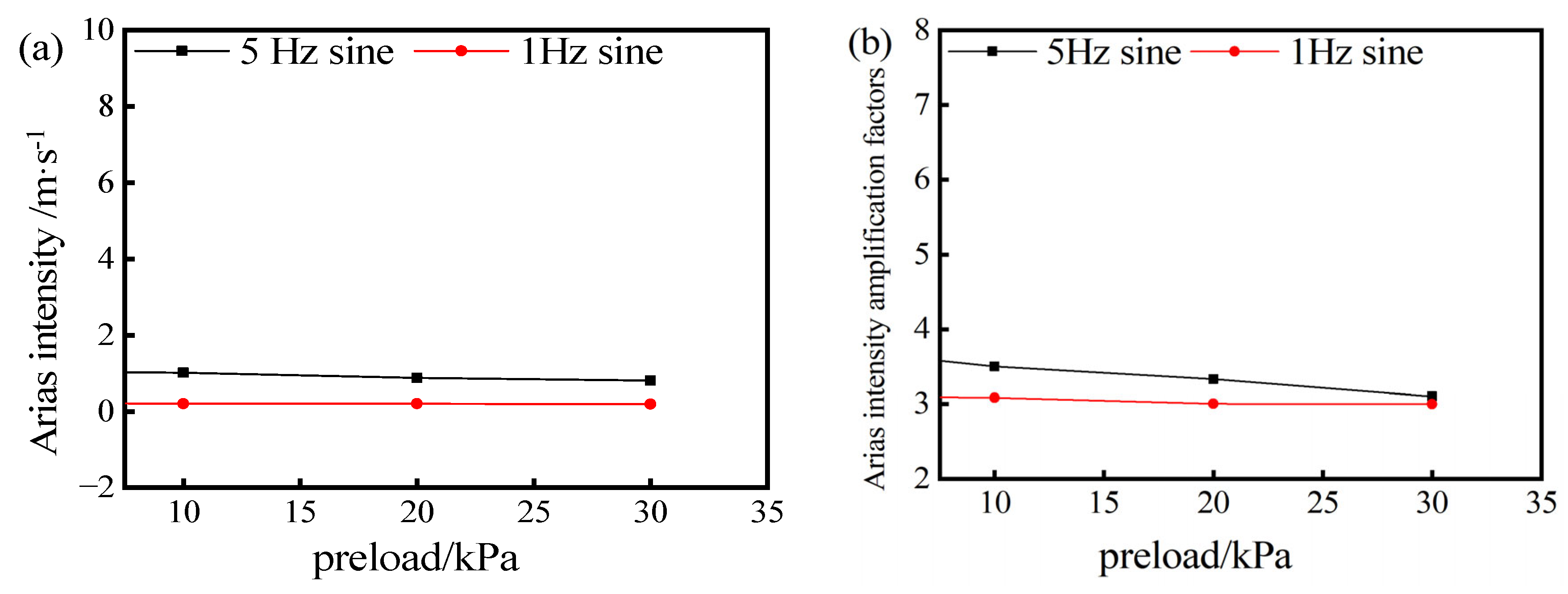
Graphical analysis of the site’s Arias intensity (see Figure 19) shows that the Arias intensity amplification factors for 1 Hz and 5 Hz sine waves exceed 3.0, whereas the ground motion amplification factor factors stay below 3.0. This indicates that the model site amplifies Arias intensity more than peak acceleration. The trends in the Arias amplification factor and the peak ground acceleration amplification factor with consolidation pressure are closely aligned, peaking at lower consolidation pressures, and decreasing as consolidation pressure increases.
Based on this study, it can be inferred that, as the site’s predominant period approaches or deviates from the principal period of the seismic waves, the site’s response will either intensify or weaken. Changes in consolidation pressure alter the site’s predominant period, which consequently amplifies or reduces the impact of seismic waves. We speculate that this is caused by changes in soil conditions, such as the voids in the soil. The experimental results of this paper reveal that the ground response at SBR sites is strongly influenced by the site’s dominant period and the primary period of the seismic waves.
5. Conclusions
To explore the seismic response characteristics of blown sand reclamation sites, we designed and validated a specialized, layered shear box. We conducted a series of shaking-table experiments to measure parameters like the site’s predominant period and ground motion amplification factor, and to examine their interrelationship. The key findings are summarized below:
- (1)
- The stratified shearing model box experiences minimal boundary effects. Under the test conditions of inputting a 1 Hz sine wave with an acceleration amplitude of 0.05 g, and a 5 Hz sine wave with an acceleration amplitude of 0.05 g, the influence factor DA (%) of the box boundaries on the top and middle soil layers varied from 3.27% to 5.78%.
- (2)
- The loading system was effective in maintaining pressure and settlement close to the predetermined values, with minimal impact of load variation during the experiments. When pressures of 10, 20, and 30 kPa were applied by the loading system, the model soil experienced maximum settlements of −15.963, −31.436, and −39.265 mm, respectively. After the release of pressure, the soil rebound was measured to be 1.653, 3.626, and 4.634 mm, respectively.
- (3)
- Changes in consolidation pressure and soft soil properties lead to shifts in the site’s predominant period. As the consolidation pressure in the soil layer increases from 0 kPa to 30 kPa, the predominant period decreases from 0.181 s to 0.131 s. At the same consolidation pressures, the predominant period of the sand soil layer is shorter compared to the entire site. This suggests that the presence of soft-soil layers shifts the site’s predominant period towards longer durations.
- (4)
- When the period of the input wave aligns with the site’s period, resonance occurs, amplifying seismic vibrations. As the period diverges from the site’s predominant period, the resonance effect weakens. At 0 kPa consolidation pressure, the site’s predominant period is 0.181 s, closely aligning with the 5 Hz sine period. This alignment maximizes both the ground motion amplification factor and the Arias intensity amplification factor. As consolidation pressure increases and the input wave’s period further diverges from the site’s predominant period, both the ground motion amplification factor and the Arias intensity amplification factor exhibit a decreasing trend.
Author Contributions
Methodology, J.L. and Y.Y.; Validation, J.L.; Formal analysis, J.L.; Investigation, X.L.; Resources, Y.G.; Writing—original draft, J.L.; Writing—review & editing, Y.W.; Project administration, T.L. All authors have read and agreed to the published version of the manuscript.
Funding
This research received no external funding.
Data Availability Statement
The original contributions presented in the study are included in the article, further inquiries can be directed to the corresponding authors.
Acknowledgments
The authors would like to thank The Key Laboratory of Disaster Prevention and Structural Safety at Guangxi University, China, supporting this project. Moreover, the authors would like to thank Dong Zhou from Guangxi University for their valuable guidance.
Conflicts of Interest
Author Yi Wei was employed by the company Nnaning Newhope Real Estate Co., Ltd. Author Yuanfang Yan was employed by the company Guangxi Xinfazhan Communication Group Co., Ltd. The remaining authors declare that the research was conducted in the absence of any commercial or financial relationships that could be construed as a potential conflict of interest.
References
- Işık, E. Structural failures of adobe buildings during the February 2023 Kahramanmaraş (Türkiye) earthquakes. Appl. Sci. 2023, 13, 8937. [Google Scholar] [CrossRef]
- Essar, M.Y.; Wahdati, S.; O’Sullivan, B.; Nemat, A.; Blanchet, K. Cycles of disasters in Afghanistan: The urgent call for global solidarity. PLoS Glob. Public Health 2024, 4, e0002751. [Google Scholar] [CrossRef] [PubMed]
- Yeck, W.L.; Hatem, A.E.; Goldberg, D.E.; Barnhart, W.D.; Jobe, J.A.T.; Shelly, D.R.; Villaseñor, A.; Benz, H.M.; Earle, P.S. Rapid Source Characterization of the 2023Mw 6.8 Al Haouz, Morocco, Earthquake. Seism. Rec. 2023, 3, 357–366. [Google Scholar] [CrossRef]
- Singh, S.K.; Mena, E.A.; Castro, R. Some aspects of source characteristics of the 19 September 1985 Michoacan earthquake and ground motion amplification in and near Mexico City from strong motion data. Bull. Seismol. Soc. Am. 1988, 78, 451–477. [Google Scholar]
- Campillo, M.; Gariel, J.C.; Aki, K.; Sánchez-Sesma, F.J. Destructive strong ground motion in Mexico City: Source, path, and site effects during great 1985 Michoacán earthquake. Bull. Seismol. Soc. Am. 1989, 79, 1718–1735. [Google Scholar] [CrossRef]
- Housner, G.W.; Thiel, C.C. Competing against time: Report of the Governor’s Board of Inquiry on the 1989 Loma Prieta earthquake. Earthq. Spectra 1990, 6, 681–711. [Google Scholar] [CrossRef]
- Mitchell, D.; Tinawi, R.; Sexsmith, R. Performance of bridges in the 1989 Loma Prieta earthquake—Lessons for Canadian designers. Can. J. Civ. Eng. 1991, 18, 711–734. [Google Scholar] [CrossRef]
- Mitchell, D.; Tinawi, R.; Redwood, R. Damage to buildings due to the 1989 Loma Prieta earthquake—A Canadian code perspective. Can. J. Civ. Eng. 1990, 17, 813–834. [Google Scholar] [CrossRef]
- Anderson, J.G.; Bodin, P.; Brune, J.N.; Prince, J.; Singh, S.K.; Quaas, R.; Onate, M. Strong ground motion from the Michoacan, Mexico, earthquake. Science 1986, 233, 1043–1049. [Google Scholar] [CrossRef]
- Jaimes, M.A.; Lermo, J.; García-Soto, A.D. Ground-motion prediction model from local earthquakes of the Mexico basin at the hill zone of Mexico City. Bull. Seismol. Soc. Am. 2016, 106, 2532–2544. [Google Scholar] [CrossRef]
- Gülü, A. A Compendious Review on the Determination of Fundamental Site Period: Methods and Importance. Geotechnics 2023, 3, 71. [Google Scholar] [CrossRef]
- Chu, J.; Bo, M.W.; Arulrajah, A. Soil improvement works for an offshore land reclamation. Proc. Inst. Civ. Eng. Geotech. Eng. 2009, 162, 21–32. [Google Scholar] [CrossRef]
- Noda, T.; Nakai, K.; Asaoka, A. Seismic response analysis of a coastal artificial reclaimed ground containing a soft layer. IOP Conf. Ser. Mater. Sci. Eng. 2010, 10, 012107. [Google Scholar] [CrossRef]
- Vitale, S.; Isaia, R.; Ciarcia, S.; Giuseppe, M.G.; Iannuzzi, E.; Prinzi, E.; Tramparulo, F.; Troiano, A. Seismically Induced Soft-Sediment Deformation Phenomena During the Volcano-Tectonic Activity of Campi Flegrei Caldera (Southern Italy) in the Last 15 kyr. Tectonics 2019, 38, 1999–2018. [Google Scholar] [CrossRef]
- Ovando-Shelley, E.; Romo, M.P.; Contreras, N.; Giralt, A. Effects on soil properties of future settlements in downtown Mexico City due to ground water extraction. Geofísica Int. 2003, 42, 185–204. [Google Scholar] [CrossRef]
- Lermo, J.; Chávez-García, F.J. Site effect evaluation at Mexico City: Dominant period and relative amplification from strong motion and microtremor records. Soil Dyn. Earthq. Eng. 1994, 13, 413–423. [Google Scholar] [CrossRef]
- Alam, M.J.; Azad, A.; Rahman, Z. Prediction of Liquefaction Potential of Dredge Fill Sand by DCP and Dynamic Probing. AIP Conf. Proc. 2008, 1020, 296–303. [Google Scholar]
- Hu, J.; Liu, Y.; Yao, K.; Wei, H. Observation of Reinforcement Methods in Organic Disseminated Sand. In Proceedings of the International Conference on Transportation & Mechanical & Electrical Engineering (ICTMEE 2017), Qingdao, China, 9–12 June 2017. [Google Scholar]
- Lv, J.; Yin, Y.; Yu, Z.; Xu, Z.C.; Chen, G.F.; Yang, F. Study on Light Dynamic Penetration to Test Coarse Sand Relative Density in Bridge Culvert Back Sand Filling. In Proceedings of the International Conference on Transportation & Mechanical & Electrical Engineering (ICTMEE 2017), Qingdao, China, 9–12 June 2017. [Google Scholar]
- Kim, H.; Prezzi, M.; Salgado, R. Use of Dynamic Cone Penetration and Clegg Hammer Tests for Quality Control of Roadway Compaction and Construction; Joint Transportation Research Program: West Lafayette, IN, USA, 2010. [Google Scholar]
- Li, Y.; Cui, J.; Guan, T.; Jing, L. Investigation into dynamic response of regional sites to seismic waves using shaking table testing. Earthq. Eng. Eng. Vib. 2015, 14, 411–421. [Google Scholar] [CrossRef]
- Dietz, M.; Wood, D.M. Shaking table evaluation of dynamic soil properties. In Proceedings of the 4th International Conference on Earthquake Geotechnical Engineering, Thessaloniki, Greece, 25–28 June 2007. [Google Scholar]
- Afacan, K.B.; Brandenberg, S.J.; Stewart, J.P. Centrifuge modeling studies of site response in soft clay over wide strain range. J. Geotech. Geoenvironmental Eng. 2013, 140, 04013003. [Google Scholar] [CrossRef]
- Wang, X.; Li, J.C. Numerical study on the boundary effect of rigid model boxes in shaking table tests in underground engineering. IOP Conf. Ser. Earth Environ. Sci. 2021, 861, 052033. [Google Scholar] [CrossRef]
- Hashemi, S.; Ehtisham, A.; Rahmani, B. Dynamic behavior of elevated and ground-supported, base-isolated, flexible, concrete cylindrical fluid containers. J. Struct. Constr. Eng. 2021, 8, 345–366. [Google Scholar]
- Chen, M.; Ouyang, M.; Guo, H.; Zou, M.; Zhang, C. A Coupled Hydrodynamic–Structural Model for Flexible Interconnected Multiple Floating Bodies. J. Mar. Sci. Eng. 2023, 11, 813. [Google Scholar] [CrossRef]
- Matsuda, T.; Goto, Y. Studies on experimental technique of shaking table test for geotechnical problem. In Proceedings of the 9th World Conference on Earthquake Engineering, Tokyo, Japan, 2–9 August 1988. [Google Scholar]
- Whitman, R.V.; Lambe, P.C. Effect of boundary conditions upon centrifuge experiments using ground motion simulation. Geotech. Test. J. 1986, 9, 61–71. [Google Scholar] [CrossRef]
- Castelli, F.; Grasso, S.; Lentini, V.; Sammito, M. Design of a Biaxial Laminar Shear Box for 1g Shaking Table Tests. Geotechnics 2022, 2, 23. [Google Scholar] [CrossRef]
- Cheng, Z.; Li, J.; Wu, C.; Zhang, T.; Du, G. Axial Compressive Performance of Steel-Reinforced UHPC-Filled Square Stainless-Steel Tube. Buildings 2022, 13, 56. [Google Scholar] [CrossRef]
- Lee, C.J.; Wei, Y.C.; Kuo, Y.C. Boundary effects of a laminar container in centrifuge shaking table tests. Int. J. Soil Dyn. Earthq. Eng. 2012, 34, 37–51. [Google Scholar] [CrossRef]
- Vo, T.; Thai, H.; Inam, F. Axial-flexural coupled vibration and buckling of composite beams using sinusoidal shear deformation theory. Arch. Appl. Mech. 2012, 82, 1391–1408. [Google Scholar] [CrossRef]
- Glogowski, P.; Rieger, M.; Sun, J.; Kuhlenkötter, B. Natural Frequency Analysis in the Workspace of a Six-Axis Industrial Robot Using Design of Experiments. Adv. Mater. Res. 2016, 1140, 345–352. [Google Scholar] [CrossRef]
- Hardin, B.O.; Drnevich, V.P. Shear modulus and damping in soils: Measurement and parameter effects (Terzaghi lecture). J. Soil Mech. Found. Div. 1972, 98, 603–624. [Google Scholar] [CrossRef]
- Dietz, M.; Wood, D.M. Shaking Table Evaluation of Dynamic Soil Properties; Springer: Berlin/Heidelberg, Germany, 2007. [Google Scholar]
- Ha, I.-S.; Olson, S.M.; Seo, M.-W.; Kim, M.-M. Evaluation of reliquefaction resistance using shaking table tests. Soil Dyn. Earthq. Eng. 2011, 31, 682–691. [Google Scholar] [CrossRef]
- Málaga-Chuquitaype, C. Strong-motion duration and response scaling of yielding and degrading eccentric structures. Earthq. Eng. Struct. Dyn. 2020, 49, 1453–1471. [Google Scholar] [CrossRef]
- Wood, D.M.; Crewe, A.; Taylor, C. Shaking table testing of geotechnical models. Int. J. Phys. Model. Geotech. 2002, 2, 1–13. [Google Scholar] [CrossRef]
- Carlos, G.; Singh, S.K. A site effect study in Acapulco, Guerrero, Mexico: Comparison of results from strong-motion and microtremor data. Bull. Seismol. Soc. Am. 1992, 82, 642–659. [Google Scholar]
- Prasad, S.K.; Towhata, I.; Chandradhara, G.P.; Nanjundaswamy, P. Shaking table tests in earthquake geotechnical engineering. Curr. Sci. 2004, 87, 1398–1404. [Google Scholar]
- Xie, L.; Zhou, Y.; Hu, C.; Yu, H. Characteristics of response spectra of long-period earthquake ground motion. Earthq. Eng. Eng. Vib. 1990, 10, 1–20. [Google Scholar]
- Avilés, J.; Pérez-Rocha, L.E. Regional subsidence of Mexico City and its effects on seismic response. Soil Dyn. Earthq. Eng. 2010, 30, 981–989. [Google Scholar] [CrossRef]
- Mayoral, J.M.; Castañón, E.; Albarrán, J. Regional subsidence effects on seismic soil-structure interaction in soft clay. Soil Dyn. Earthq. Eng.-Southampt. 2017, 103, 123–140. [Google Scholar] [CrossRef]
- Dobry, R.; Oweis, I.; Urzua, A. Simplified procedures for estimating the fundamental period of a soil profile. Bull. Seismol. Soc. Am. 1976, 66, 1293–1321. [Google Scholar]
- Cheng, C.-C.; Yu, C.-P.; Chang, H. On the Feasibility of Deriving Transfer Function from Rayleigh Wave in the Impact-Echo Displacement Waveform. Key Eng. Mater. 2004, 270–273, 1484–1491. [Google Scholar] [CrossRef]
- Lebrun, B.; Hatzfeld, D.; Bard, P.Y. Site effect study in urban area: Experimental results in Grenoble (France). Pure Appl. Geophys. 2001, 158, 2543–2557. [Google Scholar] [CrossRef]
- Yu, S.-H. Application of Parzen window in filter back projection algorithm. IOP Conf. Ser. Mater. Sci. Eng. 2018, 392, 062183. [Google Scholar] [CrossRef]
- Viti, S.; Tanganelli, M.; D’intinosante, V.; Baglione, M. Effects of soil characterization on the seismic input. J. Earthq. Eng. 2019, 23, 487–511. [Google Scholar] [CrossRef]
- Oka, F.; Sugito, M.; Yashima, A.; Furumoto, Y. Time dependent ground motion amplification at reclaimed land after the 1995 Hyogo-ken-Nanbu Earthquake. In Proceedings of the 12th World Conference on Earthquake Engineering, Auckland, New Zealand, 30 January–4 February 2000. [Google Scholar]
Figure 1.
Kahramanmaraş after the earthquake.

Figure 2.
Villages in Herat Province, western Afghanistan, after being struck by a 6.3 magnitude earthquake.
Figure 2.
Villages in Herat Province, western Afghanistan, after being struck by a 6.3 magnitude earthquake.

Figure 3.
Test system. (a) Shaking table; (b) controller computers.
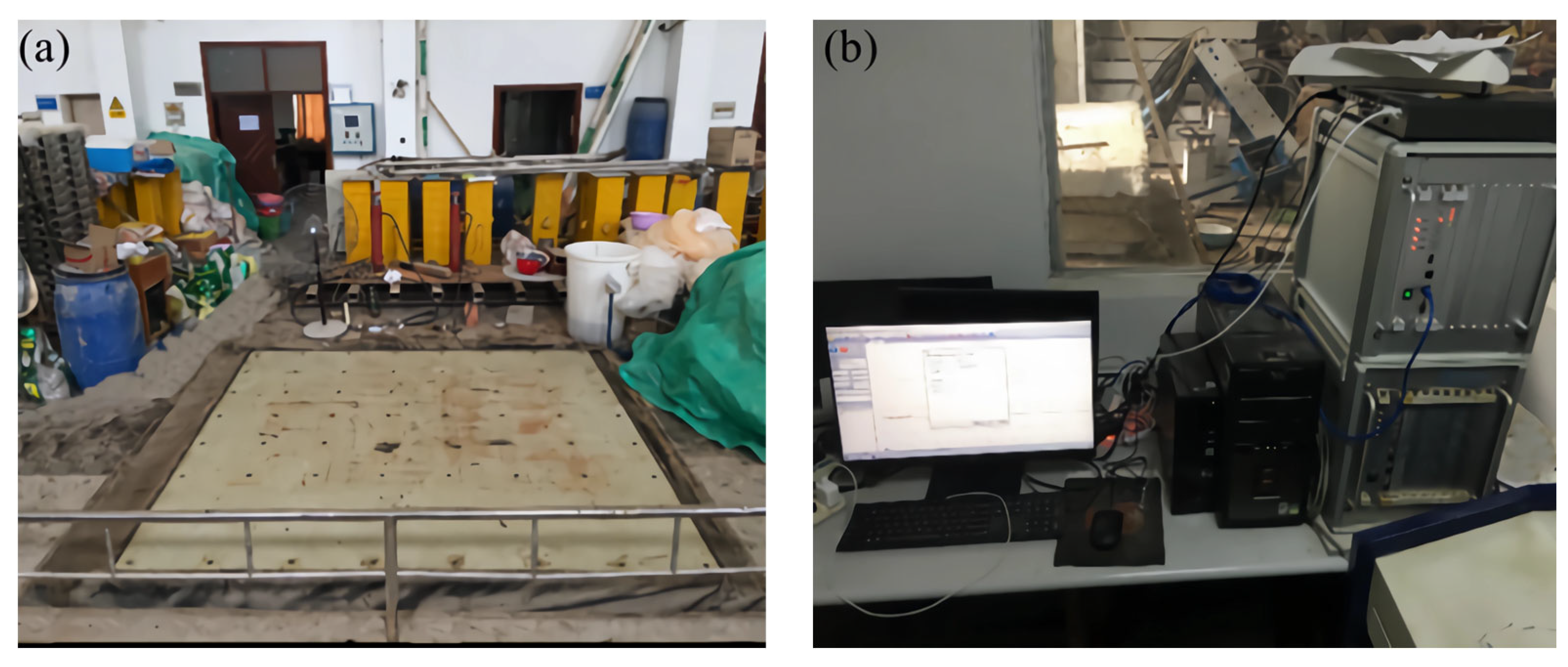
Figure 4.
Stress state: (a) soil layer model; (b) bottom frame.
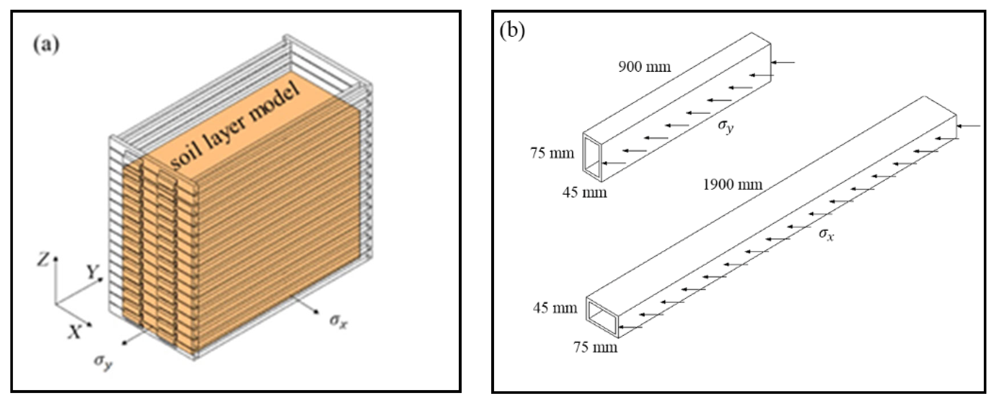
Figure 5.
Stratified shearing model box. The red rectangle indicates a bow-shaped steel plate.

Figure 6.
ANSYS model.
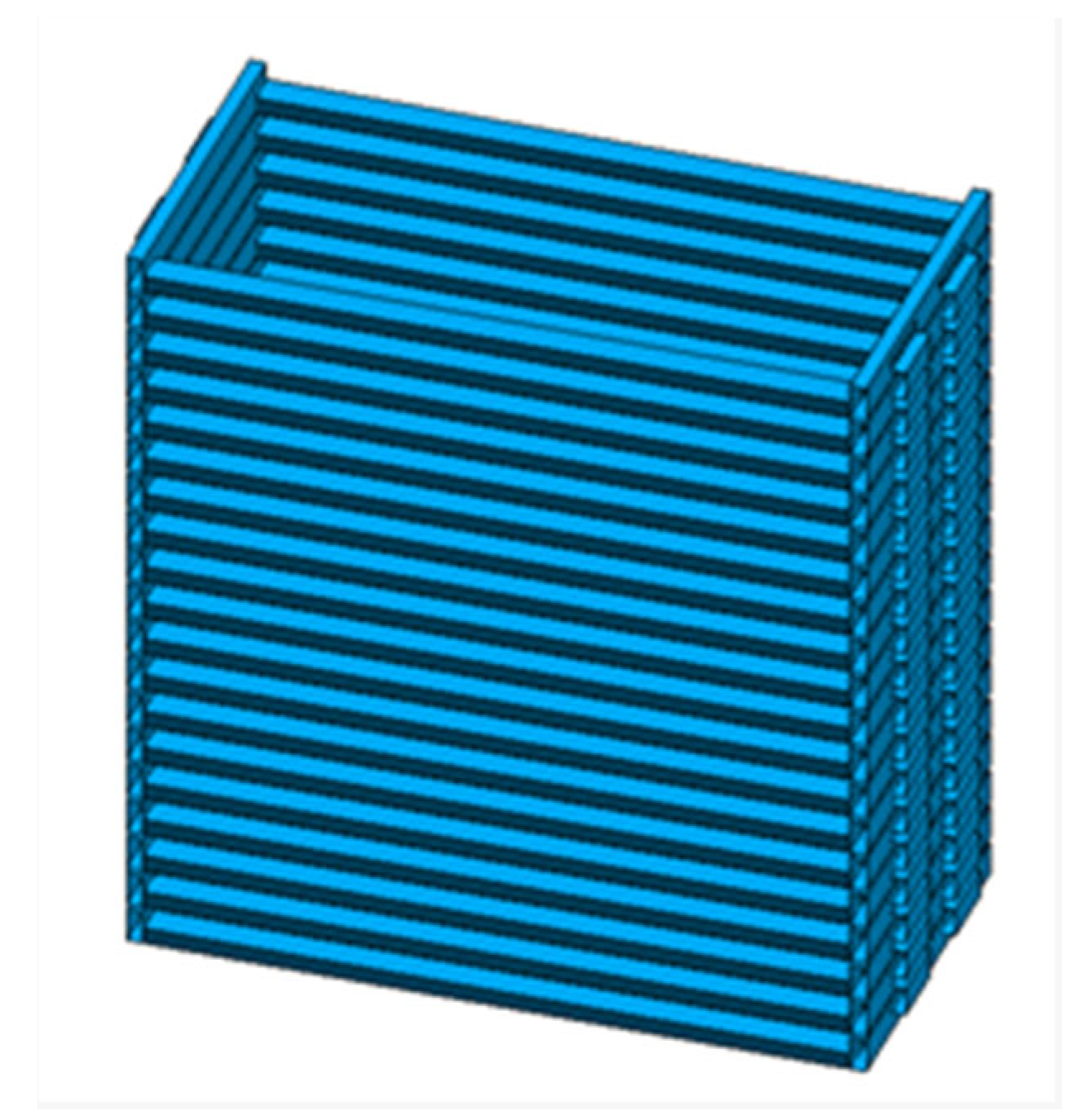
Figure 7.
Shaking table water proofer: (a) rubber layer; (b) geotextile layer.
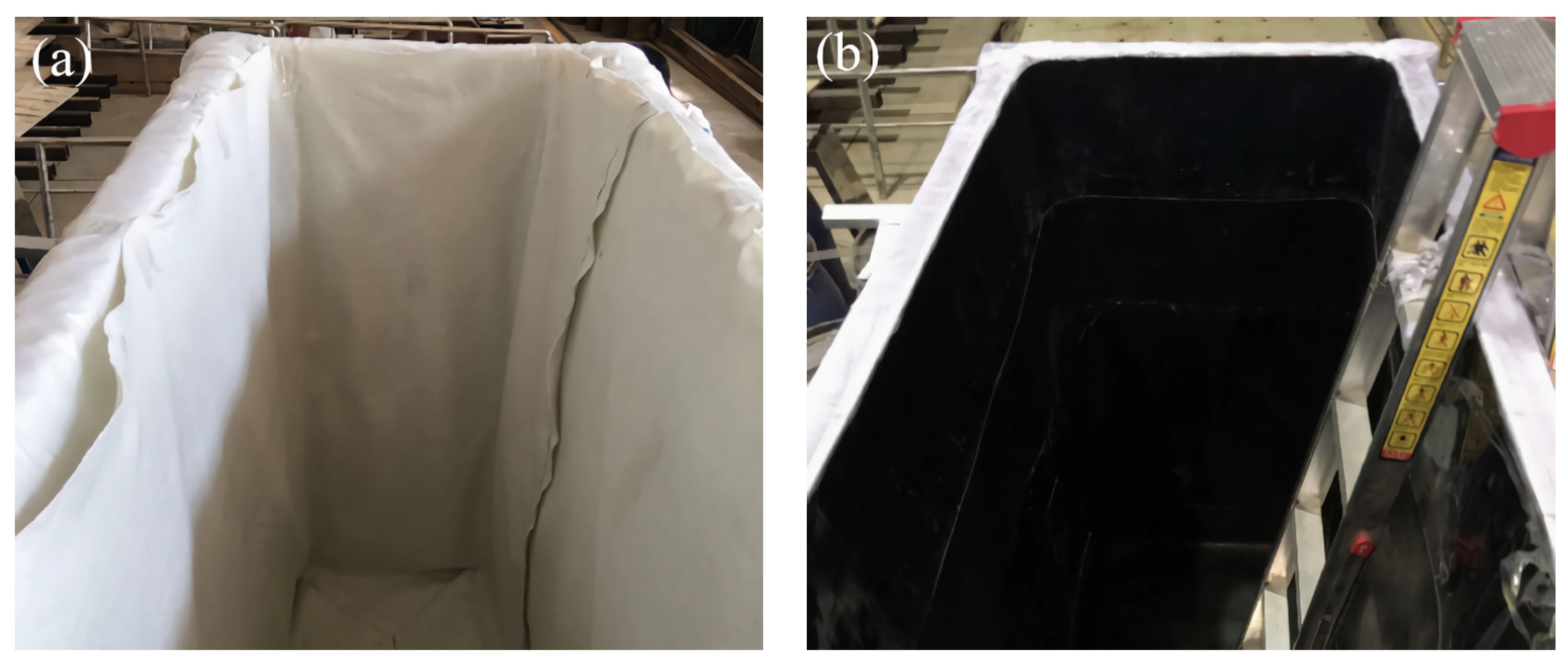
Figure 8.
Loading device design drawing.
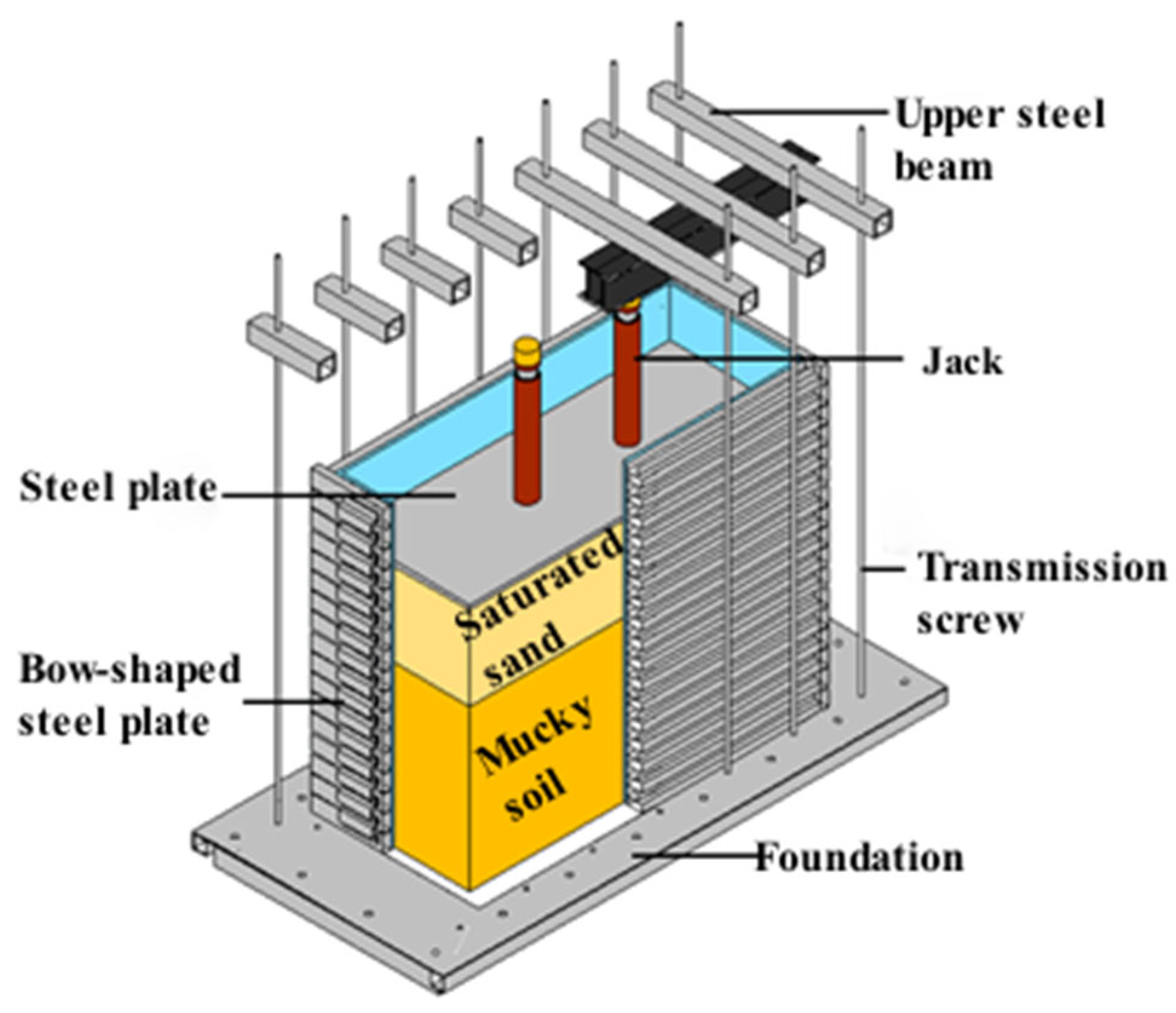
Figure 9.
Loading device actual object.
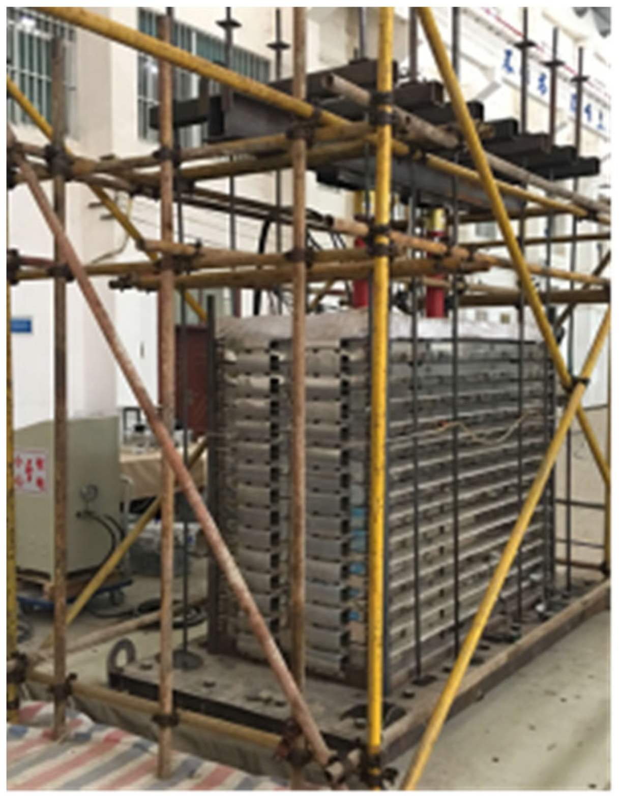
Figure 10.
Model sensor layout diagram.
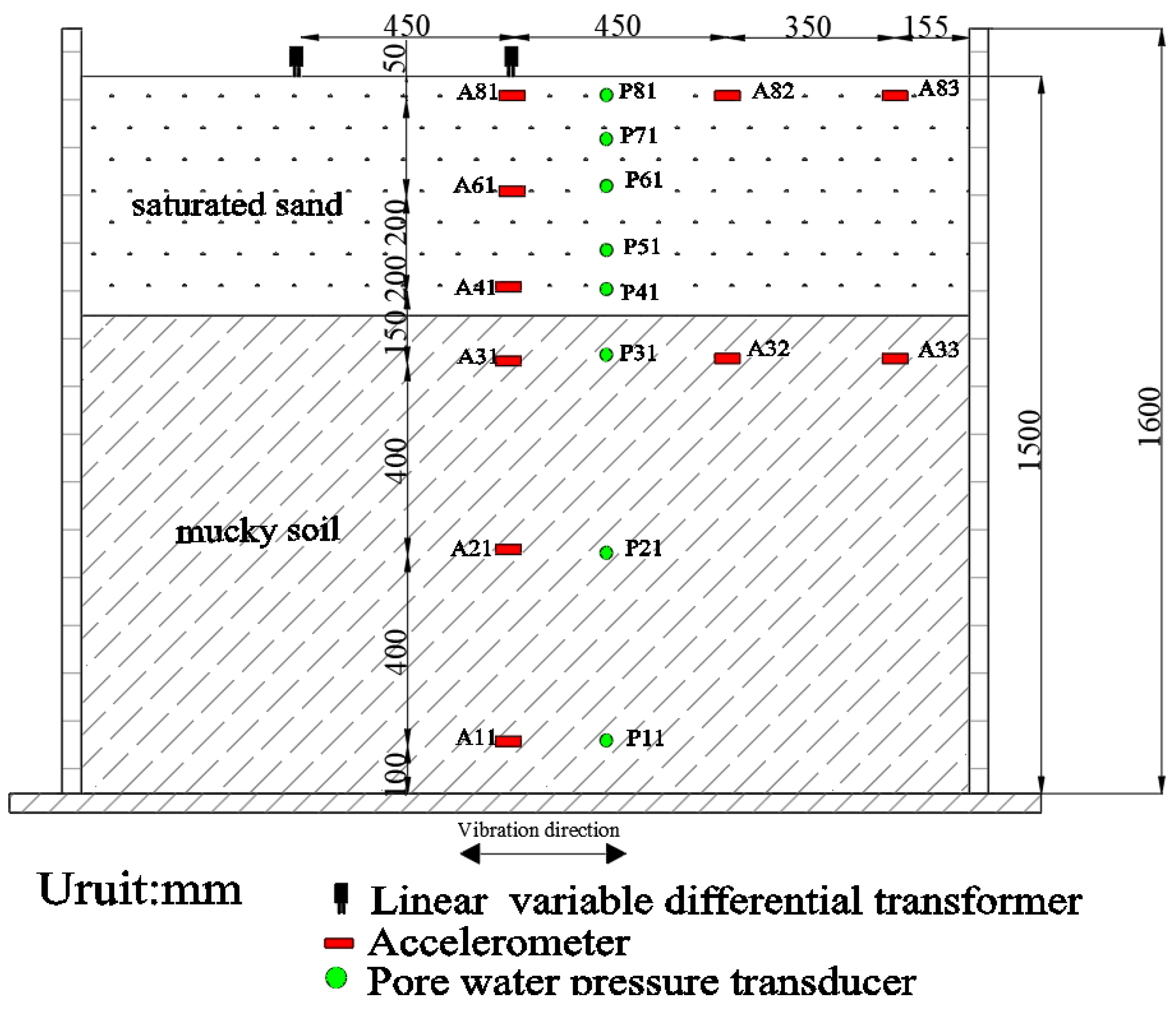
Figure 11.
Accelerometer. The inscription above the image denotes a flat-axis accelerometer.
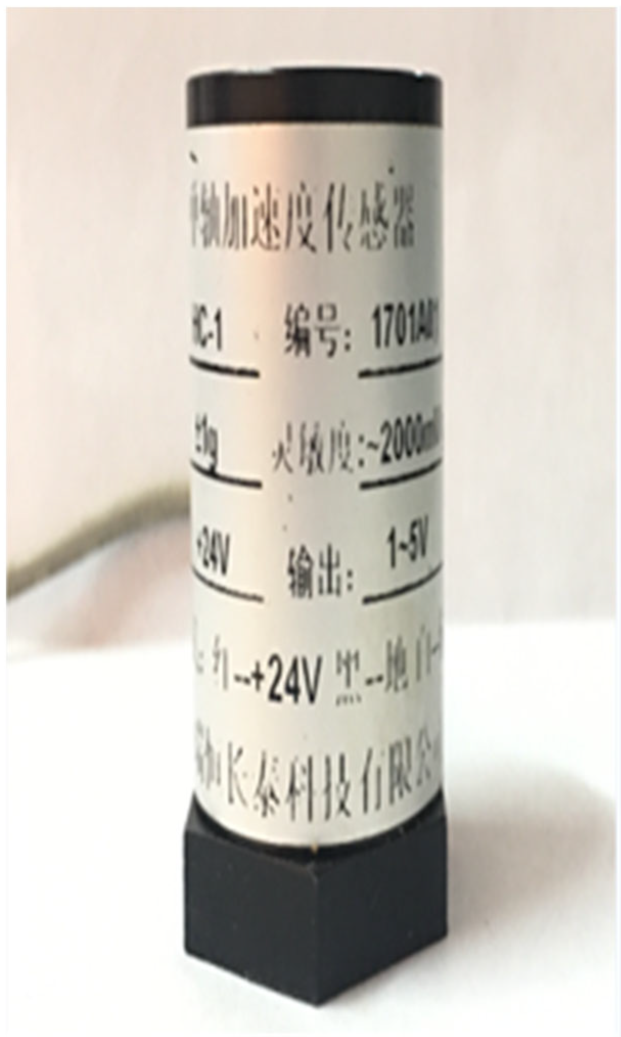
Figure 12.
Model making process: (a) reclamation of marine soft soil; (b) the settling of water injection.
Figure 12.
Model making process: (a) reclamation of marine soft soil; (b) the settling of water injection.

Figure 13.
Acceleration time histories of each sensor for a 1 Hz sine wave input. Accelerometer: (a) A81, (b) A82, (c) A83, (d) A31, (e) A32, (f) A33.
Figure 13.
Acceleration time histories of each sensor for a 1 Hz sine wave input. Accelerometer: (a) A81, (b) A82, (c) A83, (d) A31, (e) A32, (f) A33.
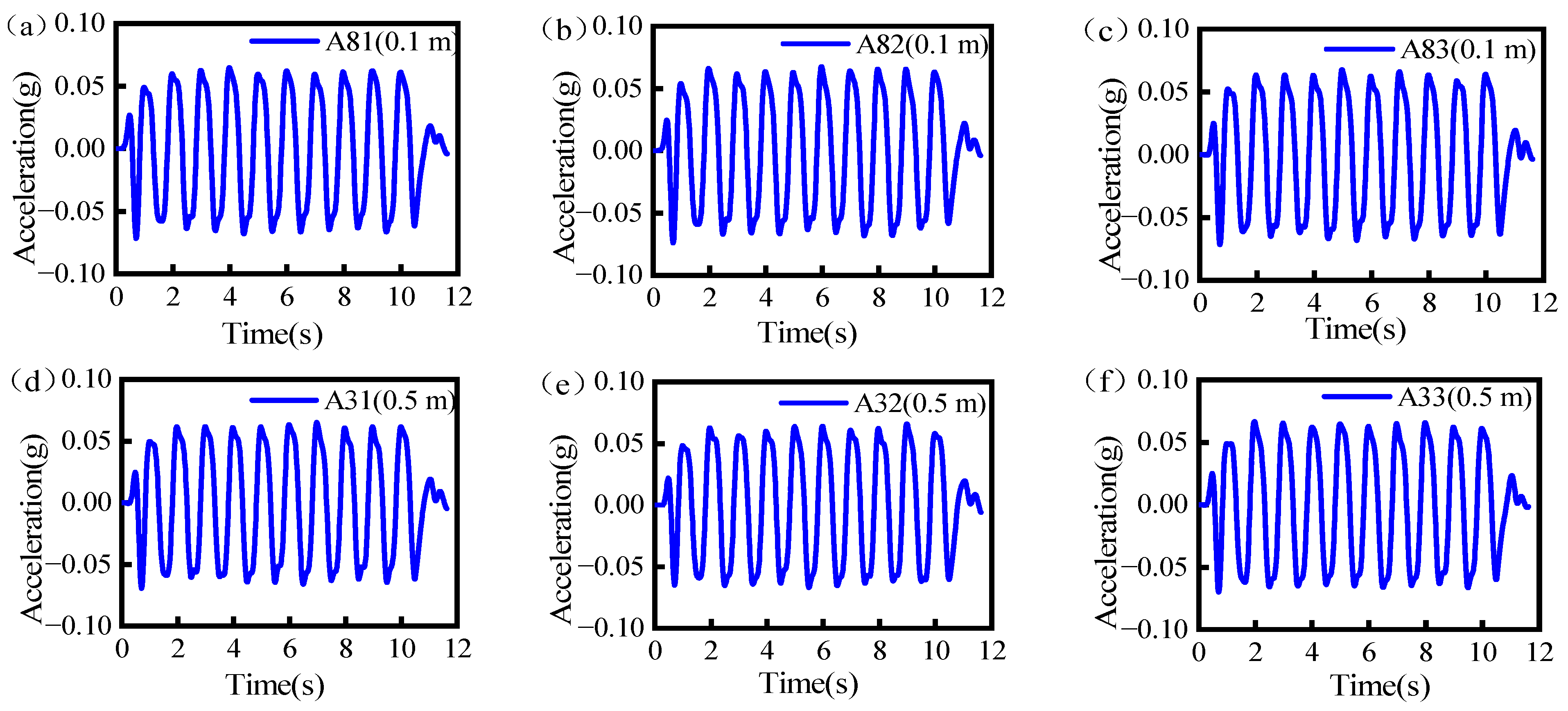
Figure 14.
The influence of the box boundary on the dynamic response of (a) the middle layer and (b) the top layer.
Figure 14.
The influence of the box boundary on the dynamic response of (a) the middle layer and (b) the top layer.

Figure 15.
Load and settlement values at the top of the soil layer during the loading test. (a) Load value; (b) settlement value.
Figure 15.
Load and settlement values at the top of the soil layer during the loading test. (a) Load value; (b) settlement value.
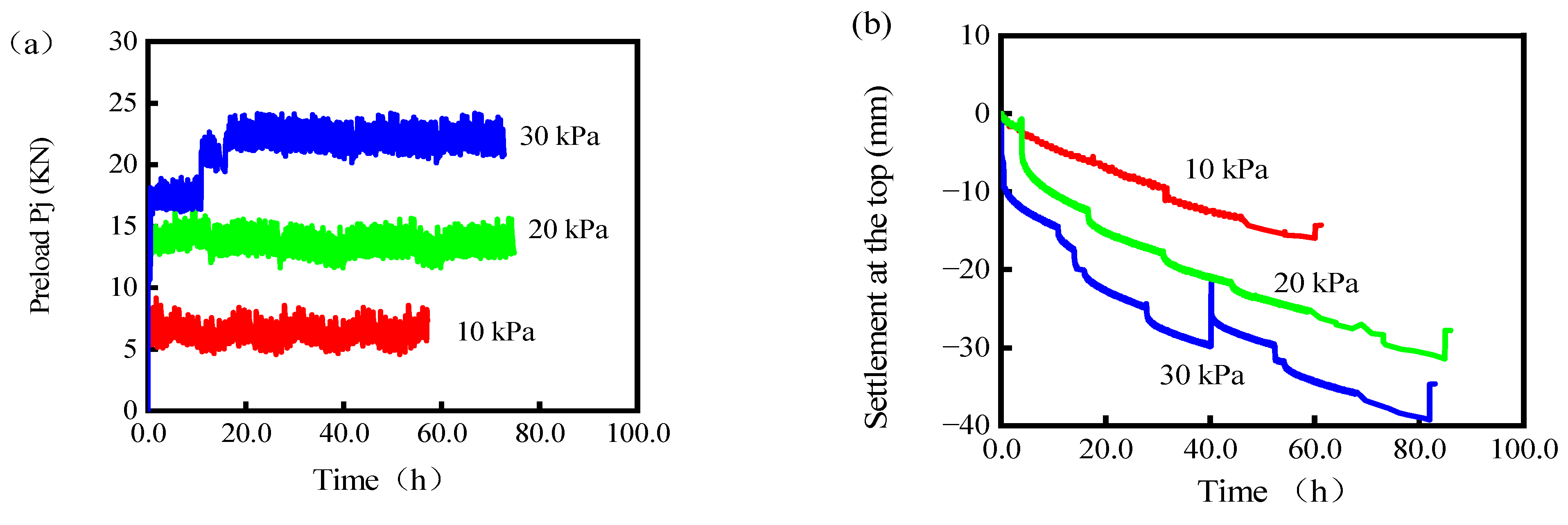
Figure 16.
Amplitude of an acceleration transfer functions of soil layers under various consolidation states. The transfer functions of the Surface (Entire site) are shown by (a,c,e,g), and the transfer functions at the soil layer interfaces (Sand soil) are shown by (b,d,f,h).
Figure 16.
Amplitude of an acceleration transfer functions of soil layers under various consolidation states. The transfer functions of the Surface (Entire site) are shown by (a,c,e,g), and the transfer functions at the soil layer interfaces (Sand soil) are shown by (b,d,f,h).
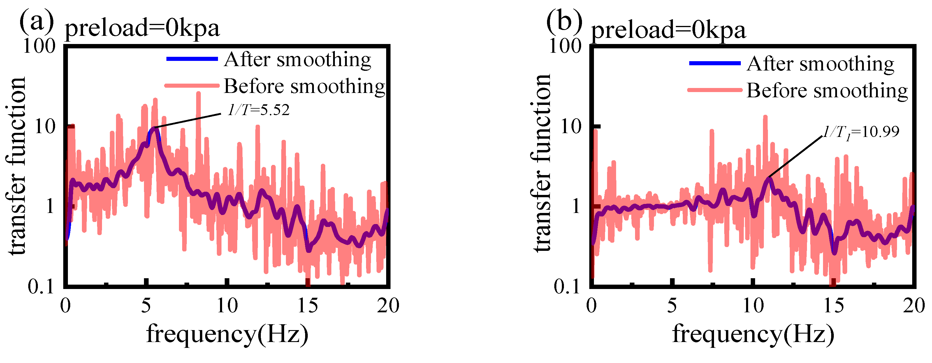
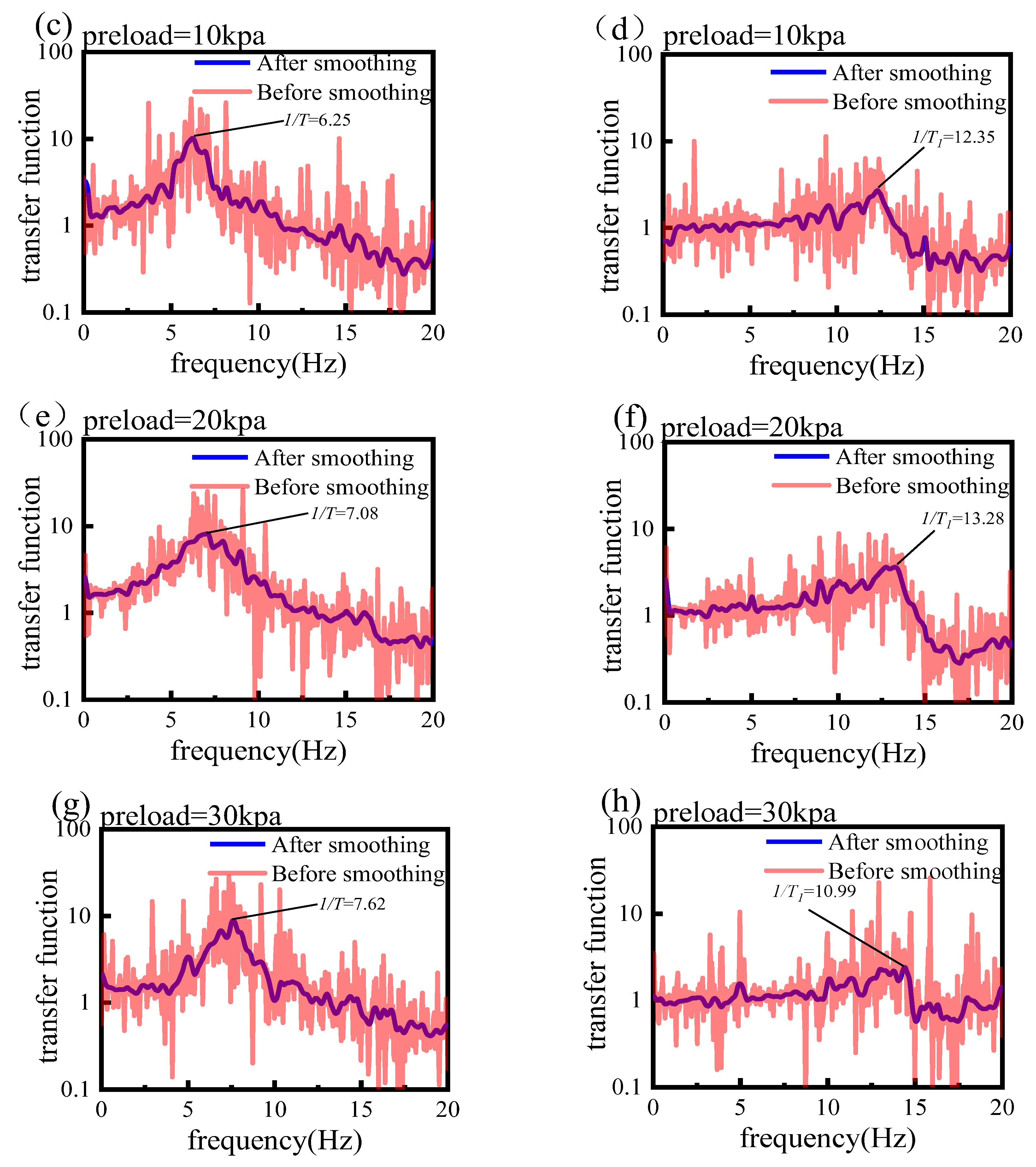
Figure 17.
Excess pore water pressure under different consolidation preloading: (a) preload = 0 kPa; (b) preload = 10 kPa; (c) preload = 20 kPa; (d) preload = 30 kPa.
Figure 17.
Excess pore water pressure under different consolidation preloading: (a) preload = 0 kPa; (b) preload = 10 kPa; (c) preload = 20 kPa; (d) preload = 30 kPa.
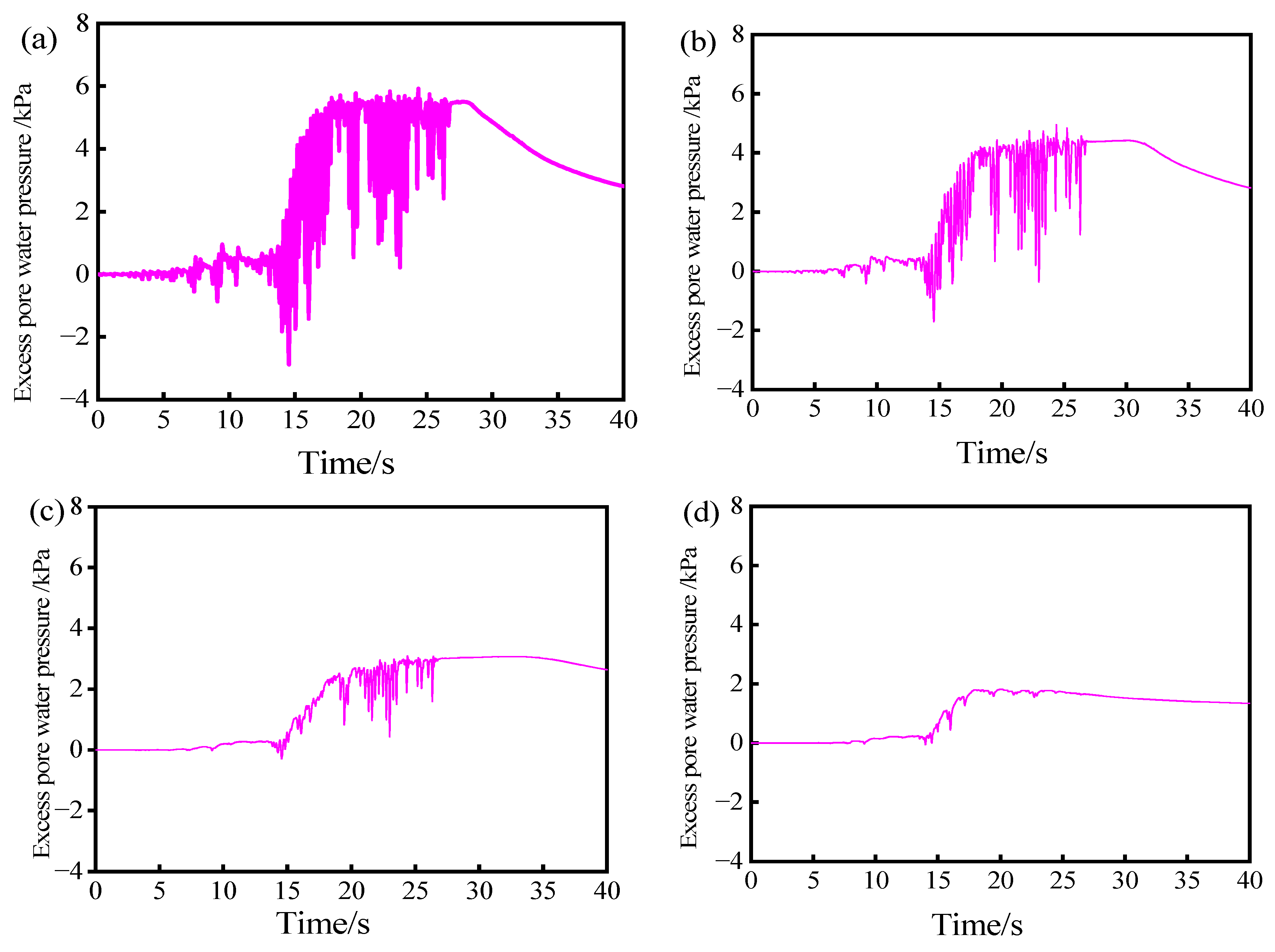
Figure 18.
(a) Peak acceleration; (b) ground motion amplification factor.
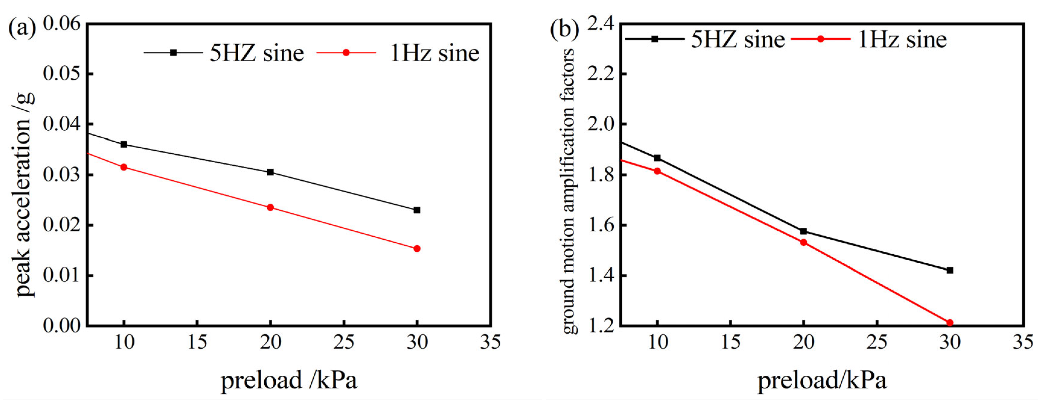
Figure 19.
(a) Arias intensity; (b) Arias intensity amplification factors.

Table 1.
Maximum tensile stress and shear stress of stainless-steel square tubes.
| Thickness/mm | 0.9 | 1 | 1.2 | 1.5 | 2 | 2.5 | 3 |
|---|---|---|---|---|---|---|---|
| Longitudinal tensile stress/MPa | 181.03 | 163.55 | 137.35 | 111.17 | 85.01 | 69.34 | 58.92 |
| Longitudinal shear stress/MPa | 17.21 | 15.50 | 12.95 | 10.40 | 7.84 | 6.31 | 5.29 |
| Short-axis tensile stress/MPa | 60.75 | 54.99 | 46.35 | 37.72 | 29.11 | 23.97 | 20.56 |
| Short-axis shear stress/MPa | 15.37 | 13.86 | 11.60 | 9.34 | 7.08 | 5.73 | 4.82 |
| Weight proportion/% | 3.77 | 4.18 | 5.01 | 6.23 | 8.27 | 10.28 | 12.26 |
Table 2.
Natural vibration frequency of model box.
| Thickness of the Steel Plate | 0.5 mm | 0.7 mm | 1.0 mm | 1.2 mm |
|---|---|---|---|---|
| First-order natural frequency of the model box/Hz | 0.7228 | 1.1800 | 1.9642 | 2.5352 |
| Second-order natural frequency of the model box/Hz | 2.1618 | 3.5284 | 5.8703 | 7.5730 |
| Third-order natural frequency of the model box/Hz | 3.5804 | 5.8416 | 9.7097 | 12.514 |
Table 3.
Physical properties of soft soil and sandy soil.
| Soft Soil | Physical Properties | Sandy Soil | Physical Properties |
|---|---|---|---|
| Moisture Content, (%) | 46.1 | Specific Gravity, (-) | 2.67 |
| Density, (g·cm−3) | 1.71 | Maximum Dry Density, (g·cm−3) | 1.702 |
| Porosity, (-) | 1.306 | Minimum Dry Density, (g·cm−3) | 1.430 |
| Liquid Limit, (%) | 44.2 | Maximum Void Ratio, (-) | 0.867 |
| Plastic Limit, (%) | 23.3 | Minimum Porosity, (-) | 0.568 |
| Permeability Coefficient, (10−6cm·s−1) | 6.653 | Relative Density | 0.558 |
Table 4.
Similitude ratio of the model.
| Variables | Dimension | Similarity Relationship | Similitude Ratio | |
|---|---|---|---|---|
| Model | Prototype | |||
| Length/l | L | Sl | 0.1 | 1 |
| Density/ρ | ML−3 | Sρ | 1 | 1 |
| Acceleration/a | LT | Sa | 1 | 1 |
| Time/t | LT | Sl1/2 × Sa−1/2 | 10−1/2 | 1 |
| Frequency/f | T−1 | Sl−1/2 × Sa1/2 | 101/2 | 1 |
| Displacement/s | L | Sl | 0.1 | 1 |
| Velocity/v | LT−1 | Sl1/2 × Sa1/2 | 10−1/2 | 1 |
| Stress/σ | ML−1T−2 | Sl × Sρ × Sa | 0.1 | 1 |
Table 5.
Test conditions.
| Experiment Number | Preload | Consolidation Time | Input Wave |
|---|---|---|---|
| Test-1 | 0 | -- | White noise 1 Hz Sine wave, 5 Hz Sine wave |
| Test-2 | 10 | 3d | White noise 1 Hz Sine wave, 5 Hz Sine wave |
| Test-3 | 20 | 5d | White noise 1 Hz Sine wave, 5 Hz Sine wave |
| Test-4 | 30 | 5d | White noise 1 Hz Sine wave, 5 Hz Sine wave |
Table 6.
Boundary effect influence factor DA (%) of the shaking table.
| Depth | Influence Factors | |||
|---|---|---|---|---|
| 1 Hz Sine Wave, Acceleration Amplitude of 0.05 g | 5 Hz Sine Wave, Acceleration Amplitude of 0.05 g | |||
| S-2 | S-3 | S-2 | S-3 | |
| 0.5 m | 3.67% | 3.27% | 5.78% | 4.45% |
| 0.1 m | 5.04% | 4.23% | 3.67% | 5.24% |
Table 7.
The natural periods and shear wave velocities of soil layers under each consolidation load.
Table 7.
The natural periods and shear wave velocities of soil layers under each consolidation load.
| Number | Preload/kPa | Predominant Periods/s | Shear Wave Velocity m/s | ||
|---|---|---|---|---|---|
| Surface (Entire Site) | Interface (Sand Soil) | Upper Layer (Sand Soil) | Bottom Layer (Soft Soil) | ||
| 1 | 0 | 0.181 | 0.091 | 26.37 | 37.33 |
| 2 | 10 | 0.160 | 0.081 | 29.65 | 42.43 |
| 3 | 20 | 0.141 | 0.075 | 31.88 | 49.34 |
| 4 | 30 | 0.131 | 0.069 | 34.57 | 52.85 |
Disclaimer/Publisher’s Note: The statements, opinions and data contained in all publications are solely those of the individual author(s) and contributor(s) and not of MDPI and/or the editor(s). MDPI and/or the editor(s) disclaim responsibility for any injury to people or property resulting from any ideas, methods, instructions or products referred to in the content. |
© 2024 by the authors. Licensee MDPI, Basel, Switzerland. This article is an open access article distributed under the terms and conditions of the Creative Commons Attribution (CC BY) license (https://creativecommons.org/licenses/by/4.0/).
Share and Cite
MDPI and ACS Style
Li, J.; Wei, Y.; Liang, T.; Yan, Y.; Gao, Y.; Lu, X. Design and Validation of a Stratified Shear Model Box for Seismic Response of a Sand-Blowing Reclamation Site. Buildings 2024, 14, 1405. https://doi.org/10.3390/buildings14051405
AMA Style
Li J, Wei Y, Liang T, Yan Y, Gao Y, Lu X. Design and Validation of a Stratified Shear Model Box for Seismic Response of a Sand-Blowing Reclamation Site. Buildings. 2024; 14(5):1405. https://doi.org/10.3390/buildings14051405
Chicago/Turabian StyleLi, Jiaguang, Yi Wei, Tenglong Liang, Yuanfang Yan, Ying Gao, and Xiaoyan Lu. 2024. "Design and Validation of a Stratified Shear Model Box for Seismic Response of a Sand-Blowing Reclamation Site" Buildings 14, no. 5: 1405. https://doi.org/10.3390/buildings14051405
Note that from the first issue of 2016, this journal uses article numbers instead of page numbers. See further details here.