Optimal Construction for Decoding 2D Convolutional Codes over an Erasure Channel

Abstract

In general, the problem of building optimal convolutional codes under a certain criteria is hard, especially when size field restrictions are applied. In this paper, we confront the challenge of constructing an optimal 2D convolutional code when communicating over an erasure channel. We propose a general construction method for these codes. Specifically, we provide an optimal construction where the decoding method presented in the bibliography is considered.

1. Introduction

Two-dimensional (2D) convolutional codes are suited for applications where data are organized in a two-dimensional grid, like images. The theory of 2D convolutional codes is a generalization of the theory of one-dimensional (1D) convolutional codes but much more involved. These codes were introduced in [1] and in [2] by Fornasini and Valcher, respectively. In [1], the authors considered 2D convolutional codes that were constituted of sequences indexed on ${\mathbb{Z}}^2$ with values in ${\mathbb{F}}^n$, where $\mathbb{F}$ was a finite field and established the algebraic properties of these codes. In [2], the authors studied 2D convolutional codes constituted of compact support sequences on ${\mathbb{Z}}^2$. An important property of a code is its distance since that measures its capacity of error correction. In [3], the authors defined the free distance of a 2D convolutional code, established an upper bound for this distance, and then presented some constructions of the 2D convolutional codes with an optimal free distance. A generalization of these codes, called nD convolutional codes, were first introduced in [4,5] and then further developed in [6,7,8]. However, decoding these kind of codes is a barely explored topic, which we will address in this paper. We will consider transmission over an erasure channel. Unlike the symmetric channel, where errors might occur randomly, over these channels the receiver knows in the transmission which symbols are erased and that the received symbols are correct. These channels are particularly suitable in communication systems like real-time streaming applications or situations where certain packets are more crucial than others. Convolutional codes are particularly convenient for erasure channels due to their ability to consider certain parts of the received data, thereby adapting the correction process to the erasure’s location.

There exist only two decoding algorithms for 2D convolutional codes over the erasure channel [9,10]. In [9], the authors made use of the parity-check matrices of the code, while the authors of [10] employed the encoders of the code.

The decoding algorithm presented in [9] considers the specific neighborhoods around erasures that would allow one to decode these erasures using 1D convolutional codes. These 1D codes are projections of the 2D convolutional code, and they are obtained by considering 1D parity-check matrices and by taking into account only some of the coefficients of a parity-check matrix that is of 2D code. However, the authors did not provide any such construction in which the corresponding 1D projections produced optimal efficiency for this decoding algorithm. In this paper, we discuss this problem and present several constructions of 2D convolutional codes whose corresponding associated 1D convolutional codes are optimal or quasi-optimal.

2. Preliminaries

In this section, we detail the main backgrounds of 1D and 2D convolutional codes that are required to contextualize the constructions introduced in this paper. We will also recall the decoding algorithm over an erasure channel that was presented in [9].

We denote, by $\mathbb{F}\left[z\right]$, the ring of polynomials in the indeterminate z and with coefficients in a finite field $\mathbb{F}$. By $\mathbb{F}[z_1,z_2]$, we denote the ring of polynomials in the two indeterminates, $z_1$ and $z_2$, with coefficients in $\mathbb{F}$.

2.1. 1D Convolutional Codes

Definition 1. 

An $(n,k)$ convolutional code $\mathcal{C}$ is an $\mathbb{F}\left[z\right]$-submodule of $\mathbb{F}{\left[z\right]}^n$ of rank k. A matrix $G\left(z\right)\in \mathbb{F}{\left[z\right]}^{n\times k}$ whose columns constitute a basis of $\mathcal{C}$ is called a generator matrix of $\mathcal{C}$, i.e.,

$$\mathcal{C}={\mathrm{Im}}_{\mathbb{F}\left[z\right]}G\left(z\right)=\{v\left(z\right)\in \mathbb{F}{\left[z\right]}^n:v\left(z\right)=G\left(z\right)u\left(z\right)for some u\left(z\right)\in \mathbb{F}{\left[z\right]}^k\}.$$

The vector $v\left(z\right)=G\left(z\right)u\left(z\right)$ is the codeword corresponding to the information sequence $u\left(z\right)$.

Given a convolutional code $\mathcal{C}$, two generator matrices of this code, $G\left(z\right)$ and $\overline{G}\left(z\right)$, are said to be equivalent. In addition, they differ by right multiplication with a unimodular matrix $U\left(z\right)$ (a $k\times k$ invertible polynomial matrix with a polynomial inverse or, equivalently, a $k\times k$ polynomial matrix with determinant in $\mathbb{F}\backslash \left\{0\right\}$), i.e.,

$$G\left(z\right)=\overline{G}\left(z\right)U\left(z\right).$$

A convolutional code is non-catastrophic when it admits a right prime generator matrix $G\left(z\right)$, i.e., if $G\left(z\right)=\overline{G}\left(z\right)X\left(z\right)$ with $\overline{G}\left(z\right)\in {\mathbb{F}}_q{\left[z\right]}^{n\times k}$ and $X\left(z\right)\in {\mathbb{F}}_q{\left[z\right]}^{k\times k}$, then $X\left(z\right)$ must be a unimodular matrix. A polynomial matrix is said to be left prime if its transpose is a right prime. Note that, since two generator matrices of a convolutional code differ by a right multiplication through a unimodular matrix, if a code admits a right prime generator matrix, then all its generator matrices are right prime and it will be called non-catastrophic code.

The degree $\delta$ of an $(n,k)$ convolutional code $\mathcal{C}$ is the maximum degree of the full-size minors of any generator matrix. Note that the degree can be computed with any generator matrix since two generator matrices of a code differ by the right multiplication of an unimodular matrix, as was previously said. A matrix $G\left(z\right)\in \mathbb{F}{\left[z\right]}^{n\times k}$ is said to be column-reduced if the sum of its column degrees is equal to the maximum degree of its full-size minors. A polynomial matrix is said to be row-reduced if its transpose is column-reduced. An $(n,k)$ convolutional code with degree $\delta$ is said to be an $(n,k,\delta )$ convolutional code.

Another important matrix associated with some convolutional codes $\mathcal{C}$ is the (full row rank $(n-k)\times n$) parity-check matrix noted as $H\left(z\right)$. This matrix is the generator matrix of the dual code of $\mathcal{C}$; therefore, we can generate $\mathcal{C}$ as its kernel as follows:

$$\begin{array}{cc}\hfill \mathcal{C}& =ke{r}_{\mathbb{F}\left[z\right]}H\left(z\right)\hfill \\ \hfill & =\left\{v\left(z\right)\in \mathbb{F}{\left[z\right]}^n|H\left(z\right)v\left(z\right)=\mathbf{0}\right\}.\hfill \end{array}$$

The parity-check matrix plays a central role in the decoding process for block codes and convolutional codes. Although there is always a parity-check matrix for a block code, this is not the case for convolutional codes. In [11], it was shown that a convolutional code admits a parity-check matrix if and only if it is non-catastrophic. Any non-catastrophic convolutional code admits a left prime and row-reduced parity-check matrix [12].

When transmitting information through erasure channels we may lose some parts of the information. Convolutional codes have been proven to be good for communication over these channels [13].

In [13], a decoding algorithm for these kinds of channels was presented, and it is based on solving linear systems of equations. Consider that we receive the codeword $v\left(z\right)={\sum }_{i=0}^j{v}_i{z}^i\in {\mathbb{F}}_q\left[z\right]$, and that $v_{i-t},\dots ,v_t$ are correct (have no erasures) but the coefficients afterward may have erasures. Let $H\left(z\right)={\sum }_{j\in \mathbb{N}}{H}_j{z}^j\in {\mathbb{F}}_q{\left[z\right]}^{(n-k)\times n}$ be a parity-check matrix of the code. We define the matrix as follows:

$${\mathfrak{H}}_j=\left(\begin{array}{ccccc}{H}_{\nu }& \cdots & H_0& & \\ & \ddots & & \ddots & \\ & & H_{\nu }& \cdots & H_0\end{array}\right)\in {\mathbb{F}}_q^{(j+1)(n-k)\times (\nu +j+1)n}.$$

(1)

Then, ${\mathfrak{H}}_j{\left(v_{t-\nu }^T\dots v_t^T\dots v_{t+j}^T\right)}^T=0$. By reordering these equations we can obtain a linear system of the form

$$H^e{v}^e=b,$$

(2)

where $H^e$ and $v^e$ are the columns of ${\mathfrak{H}}_j$ and the coordinates of ${\left(v_{t-\nu }^T\dots v_t^T\dots v_{t+j}^T\right)}^T$ that correspond with the erasures, respectively; and $b=-H^c{v}^c$, where $H^c$ and $v^c$ are analogously defined concerning the correctly received information. Therefore, we can correct the erasures by solving a linear system with as many unknowns as erasures in the received codeword. Note that we have considered only part of the coefficients of $v\left(z\right)$, i.e., the coefficients $v_{t-\nu },\dots ,v_t,\dots ,v_{t+j}$. We refer to this sequence as a window, and we say that it is a window of $j+\nu +1$ size.

Notice that, in order to correct the erasures produced in a codeword, we need a previous safe space where all coefficients are correctly recovered. In the construction of the system (2), the $\nu$ vectors, $v_{t-\nu },\dots ,v_{t-1}$—which were previous to $v_t$ and the first coefficient of $\widehat{\mathbf{v}}\left(z\right)$ with some erasure—conformed to this safe space.

Once we have a method for correcting the erasures produced by a channel, we may want to know the correction capability that a code can achieve. This capacity is described in terms of the distances of the code. For convolutional codes, there exist two different distances: the free distance and the column distance. The Hamming weight of a vector $v\left(z\right)={\sum }_{i\in {\mathbb{N}}_0}{v}_i{z}^i\in {\mathbb{F}}_q{\left[z\right]}^n$ is given by the expression

$$wt\left(v\left(z\right)\right)=\sum _{i\in {\mathbf{N}}_0}wt\left(v_i\right),$$

where $wt\left(v_i\right)$ is the number of non-zero coordinates of $v_i$.

Definition 2. 

Let $\mathcal{C}$ be an $(n,k)$ convolutional code, then the  free distance of $\mathcal{C}$ is

$$d_{free}\left(\mathcal{C}\right)=min\{\mathrm{wt}\left(v\left(z\right)\right):v\left(z\right)\in \mathcal{C}\backslash \left\{0\right\}\}.$$

The next theorem establishes an upper bound on the free distance of a convolutional code, and it is called the generalized Singleton bound.

Theorem 1 

([14]). Let $\mathcal{C}$ be an $(n,k,\delta )$ convolutional code. Then,

$$d_{free}\left(\mathcal{C}\right)\le (n-k)\left(⌊\frac{\delta }{k}⌋+1\right)+\delta +1.$$

The free distance of a convolutional code allows us to know the correction capacity for errors and erasures once the whole codeword is received.

An advantage of convolutional codes over block codes is that they permit us to do a partial decoding, i.e., we can start recovering erasures even though we do not have the complete codeword. The measurement of the capability of this kind of correction is given by the column distances, which are defined for non-catastrophic convolutional codes [15].

Given a vector ${\displaystyle w\left(z\right)=\sum _{i\in {\mathbb{N}}_0}{w}_i{z}^i\in \mathbb{F}{\left[z\right]}^n}$ and $j_1,j_2\in {\mathbb{N}}_0$ with $j_1<j_2$, we defined the truncation of $w\left(z\right)$ to the interval $[j_1,j_2]$ as $w_{[j_1,j_2]\left(z\right)}=w_{j_1}{z}^{j_1}+w_{j_1+1}{z}^{j_1+1}+\cdots +w_{j_2}{z}^{j_2}$.

Definition 3. 

Let $\mathcal{C}$ be an $(n,k,\delta )$ non-catastrophic convolutional code, then the j-column distance of $\mathcal{C}$ is defined by

$$d_j^c=min\{v_{[0,j]\left(z\right)}:v\left(z\right)\in \mathcal{C} with v \left(0\right)\ne 0\}.$$

The following inequalities can be directly deduced from the previous definitions [15]:

$$d_0^c\le d_1^c\le \cdots \le li{m}_{j\to }{d}_j^c=d_{free}\left(\mathcal{C}\right).$$

(3)

In addition to the free distance having a bound, the column distances also have a Singleton-like bound, which is given by the following theorem.

Theorem 2 

([15]). Let $\mathcal{C}$ be an $(n,k,\delta )$ non-catastrophic convolutional code. Then, for $j\in {\mathbb{N}}_0$, we have

$$d_j^c\le (n-k)(j+1)+1.$$

Moreover, if $d_j^c=(n-k)(j+1)+1$ for some $j\in {\mathbb{N}}_0$, then $d_i^c=(n-k)(i+1)+1$ for $i\le j$.

As seen in (3), the column distances cannot be greater than the free distance. In fact, there exists an integer

$$L=⌊\frac{\delta }{k}⌋+⌊\frac{\delta }{n-k}⌋$$

for which $d_j^c$ can be equal to $(n-k)(j+1)+1$, i.e., the bound can be held for $j\le L$ and $d_j^c<(n-k)(j+1)+1$, as well as for $j>L$ [15]. An $(n,k,\delta )$ convolutional code with $d_j^c=(n-k)(j+1)+1$ for $j\le L$ (or equivalently with $d_L^c=(n-k)(L+1)+1$) is called a maximum distance profile (MDP) code. Next, we detail a characterization of these codes in terms of their generator and parity-check matrices. For that, we need the definition of a superregular matrix.

The determinant of a square matrix $A=\left[{\mu }_{i,\ell }\right]$ over a field $\mathbb{F}$ is given by

$$\left|A\right|=\sum _{\sigma \in S_m}{(-1)}^{sgn\left(\sigma \right)}{\mu }_{1,\sigma \left(1\right)}{\mu }_{2,\sigma \left(2\right)}\cdots {\mu }_{m,\sigma \left(m\right)},$$

where $S_m$ is the symmetric group. We will refer to term as the addends of $\left|A\right|$, that is, to the product of the form ${\mu }_{1,\sigma \left(1\right)}{\mu }_{2,\sigma \left(2\right)}\cdots {\mu }_{m,\sigma \left(m\right)}$ and as a component of the factor of a term, i.e., the multiplicands of the form ${\mu }_{i,\mu \left(i\right)}$ for $i\in \{1,\dots ,m\}$. We will also say that a term is trivial if at least one of its components is zero, that is, the term is zero. Now, let A be a square submatrix of a matrix B; if all the terms of $\left|A\right|$ are trivial, then we say that $\left|A\right|$ is a trivially zero minor of B or that it is a trivial minor of B.

Definition 4 

([16,17]). Let $n,m\in \mathbb{N}$ and $B\in {\mathbb{F}}^{n\times m}$, then B is superregular if all of its non-trivial zero minors are non-zero.

Theorem 3 

([15]). Let $\mathcal{C}$ be a non-catastrophic convolutional code with a right prime and column-reduced generator matrix $G\left(z\right)={\sum }_{i=0}^{\mu }{G}_i{z}^i\in {\mathbb{F}}_q{\left[z\right]}^{n\times k}$, as well as a left prime and row-reduced parity-check matrix $H\left(z\right)={\sum }_{i=0}^{\nu }{H}_i{z}^i\in {\mathbb{F}}_q{\left[z\right]}^{(n-k)\times n}$, then the following statements are equivalent:

1. 

$\mathcal{C}$ is an MDP code

2. 

$\mathcal{G}≔\left[\begin{array}{ccc}{G}_0& \cdots & G_L\\ & \ddots & ⋮\\ & & G_0\end{array}\right]$, where $G_i=0$ for $i>\mu$, and it also has the property that every full-size minor that is not trivially zero is non-zero.

3. 

$\mathcal{H}≔\left[\begin{array}{cc}{H}_0& \\ ⋮& \ddots & \\ H_L& \cdots & H_0\end{array}\right]$, where $H_i=0$ for $i>\nu$, and it also has the property that every full-size minor that is not trivially zero is non-zero.

Lemma 1 

([13]). Let $\mathcal{C}$ be an $(n,k,\delta )$ MDP convolutional code. If any sliding window of length $(j_0+1)n$ at most $(j_0+1)(n-k)$ erasures occur with $j_0\in \{0,1,\dots ,L\}$, then we can completely recover the transmitted sequence.

This family of optimal codes requires a great deal of regularity in the sense of the previous theorem, and this causes the construction of the MDP convolutional codes to usually require big base fields. From the applied point of view, this is a concern. In last few years, the efforts of the community have been directed to improving this situation by either giving different constructions [18,19,20,21] or finding bounds [22,23]. Research has also led to the development of MDP convolutional codes over finite rings [24].

When MDP codes cannot perform a correction due to the accumulation of erasures, we have to consider some of the packets to be lost and to continue until a safe space is found again. To solve this situation, in [13,25,26,27], a definition for Reverse-MDP convolutional codes was provided. While the usual MDP convolutional codes can only carry out a forward correction, i.e., their decoding direction is from left to right, the reverse-MDP codes will allow a backward correction, i.e., a correction from right to left.

Proposition 1 

([26], Prop 2.9). Let $\mathcal{C}$ be an $(n,k,\delta )$ convolutional code with a right prime and column-reduced generator matrix $G\left(z\right)$. Let $\overline{G}\left(z\right)$ be the matrix obtained by replacing each entry $g_{ij}\left(z\right)$ of $G\left(z\right)$ with $\overline{g_{i,j}}≔z^{{\delta }_j}{g}_{i,j}\left(z^{-1}\right)$, where ${\delta }_j$ is the i-th column degree of $G\left(z\right)$. Then, $\overline{G}\left(z\right)$ is a right prime, and column-reduced generator matrix of an $(n,k,\delta )$ convolutional code $\overline{\mathcal{C}}$ and

$$v_0+z_{1}z+\cdots +v_s{z}^s\in \mathcal{C}\iff v_s+z_{s-1}z+\cdots +v_0{z}^s\in \overline{\mathcal{C}}.$$

We call $\overline{\mathcal{C}}$ the reverse code of $\mathcal{C}$. Similarly, we denote the parity-check matrix of $\overline{\mathcal{C}}$ by $\overline{H}\left(z\right)={\sum }_{i=0}^{\nu }{\overline{H}}_i{z}^i$.

Definition 5. 

Let $\mathcal{C}$ be an MDP $(n,k,\delta )$ convolutional code. We can then say that $\mathcal{C}$ is a reverse-MDP convolutional code if the reverse code $\overline{\mathcal{C}}$ is also an MDP code.

In [13], it was proven that reverse-MDP codes can perform a correction from right to left as efficiently as an MDP code does in the opposite direction. However, to perform a backward correction, a safe space is required on the right side of the erasures. This can be easily seen in the following example.

Example 1. 

Let us assume that we are communicating through an erasure channel. If so, then we have recovered the information correctly up to an instant t and we can later receive the following pattern:

$$\begin{array}{cc}\hfill & \stackrel{\left(A\right)14}{\overbrace{★★\cdots ★}}\stackrel{\left(B\right)108}{\overbrace{\mathbf{v}\mathbf{v}★★\mathbf{v}\mathbf{v}★★\cdots \mathbf{v}\mathbf{v}★★\hspace{1em}}}|\stackrel{\left(C\right)122}{\overbrace{\mathbf{v}\mathbf{v}\cdots \mathbf{v}}}|\hfill \\ \hfill & \stackrel{\left(D\right)50}{\overbrace{★★\cdots ★}}\stackrel{\left(E\right)38}{\overbrace{\mathbf{v}\mathbf{v}\cdots \mathbf{v}}}\stackrel{\left(F\right)34}{\overbrace{★★\cdots ★}}|\stackrel{\left(G\right)122}{\overbrace{\mathbf{v}\mathbf{v}\cdots \mathbf{v}}}\dots ,\hfill \end{array}$$

where ★ indicates that the corresponding component has been erased and $\mathbf{v}$ means that the component has been correctly received. If we use a $(2,1,30)$ MDP convolutional code, we cannot perform a correction due to the accumulation of erasures at the beginning of the sequence. Nevertheless, if we consider a $(2,1,30)$ reverse-MDP convolutional code and take the first 60 symbols of $\left(C\right)$ as a safe space, then we can correct the erasures in $\left(B\right)$. We can repeat this method by taking the first 60 symbols in $\left(G\right)$ and recovering the section $\left(F\right)$, that is, we build the linear system as in (2) by considering the following sets of symbols:

$$\begin{array}{c}\hfill \stackrel{\left(B\right)108}{\overbrace{\mathbf{v}\mathbf{v}★★\mathbf{v}\mathbf{v}★★\cdots \mathbf{v}\mathbf{v}★★\hspace{1em}}}|\stackrel{\left(C\right)60}{\overbrace{\mathbf{v}\mathbf{v}\cdots \mathbf{v}}},\\ \hfill and\stackrel{\left(E\right)34}{\overbrace{\mathbf{v}\mathbf{v}\cdots \mathbf{v}}}\stackrel{\left(F\right)34}{\overbrace{★★\cdots ★}}|\stackrel{\left(G\right)60}{\overbrace{\mathbf{v}\mathbf{v}\cdots \mathbf{v}}}.\end{array}$$

This example shows that reverse-MDP convolutional codes can perform better than MDP convolutional codes when transmitting over an erasure channel since we can exploit its backward capability correction. However, this type of approach depends on the fact that over the communication there exists a long enough sequence of symbols that have been correctly received to play the role of a safe space for any of the decoding directions. The following codes are aimed at solving the situation in which a safe space cannot be found.

Definition 6 

([13]). Let $H\left(z\right)={\sum }_{i=0}^{\nu }{H}_i{z}^i\in {\mathbb{F}}_q{\left[z\right]}^{(n-k)\times n}$ be a parity-check matrix of an $(n,k,\delta )$ convolutional code $\mathcal{C}$ and $L≔\lfloor \frac{\delta }{n-k}\rfloor +\lfloor \frac{\delta }{k}\rfloor$, then we obtain the matrix

$$\mathfrak{H}≔\left(\begin{array}{ccccc}{H}_{\nu }& \cdots & H_0& & \\ & \ddots & & \ddots & \\ & & H_{\nu }& \cdots & H_0\end{array}\right)\in {\mathbb{F}}^{(L+1)(n-k)\times (\nu +L+1)n},$$

which is called a partial parity-check matrix of $\mathcal{C}$. Moreover, $\mathcal{C}$ is said to be a  complete-MDP  convolutional code if, for any of its parity-check matrices $H\left(z\right)$, every full-size minor of $\mathfrak{H}$ that is non-trivially zero is non-zero.

Complete-MDP convolutional codes have an extra feature on top of being able to perform a correction as a MDP or as reverse-MDP convolutional codes. If, in the process of decoding the code, we cannot accomplish the correction due to the accumulation of too many erasures, it can compute a new safe space to continue with the process as soon as a correctable sequence of symbols is found.

Theorem 4 

([13], Theorem 6.6). Given a code sequence from a complete-MDP convolutional code. If, in a window of size $(\nu +L+1)n$, there are not more than $(L+1)(n-k)$ erasures, and if they are distributed in such a way that between position 1 and $sn$ and between positions $(\nu +L+1)n$ and $(\nu +L+1)n-s(n-k)$, for $s=1,2,\dots ,L+1$, i.e., there are no more than $s(n-k)$ erasures, then the full correction of all symbols in this interval will be possible. In particular, a new safe space can be computed.

For more constructions, examples, and further content on complete-MDP convolutional codes, we refer the reader to [12,13,17].

Example 2. 

Again, let us assume that we are using an erasure channel. In this case, we are not able to recover some of the previous symbols and we thus receive the following pattern:

$$\begin{array}{cc}\hfill \cdots ★★& |\stackrel{\left(A\right)14}{\overbrace{★★\cdots ★}}\stackrel{\left(B\right)21}{\overbrace{\mathbf{v}\mathbf{v}\cdots \mathbf{v}}}\stackrel{\left(C\right)12}{\overbrace{★★\cdots ★}}\stackrel{\left(D\right)28}{\overbrace{\mathbf{v}\mathbf{v}\cdots \mathbf{v}}}|\hfill \\ \hfill & \stackrel{\left(E\right)19}{\overbrace{\mathbf{v}\mathbf{v}\cdots \mathbf{v}}}\stackrel{\left(F\right)13}{\overbrace{★★\cdots ★}}\stackrel{\left(G\right)30}{\overbrace{\mathbf{v}\mathbf{v}\cdots \mathbf{v}}}\stackrel{\left(H\right)13}{\overbrace{★★\cdots ★}}\hfill \\ \hfill & |\stackrel{\left(I\right)30}{\overbrace{\mathbf{v}\mathbf{v}\cdots \mathbf{v}}}\stackrel{\left(J\right)6}{\overbrace{★★\cdots ★}}\stackrel{\left(K\right)17}{\overbrace{\mathbf{v}\mathbf{v}\cdots \mathbf{v}}}\stackrel{\left(L\right)22}{\overbrace{★★\cdots ★}}|★★\cdots .\hfill \end{array}$$

Note that, if we use a $(3,2,16)$ MDP or reverse-MDP convolutional code, we require a safe space of 48 symbols to correct the erasures in any of the directions, which we cannot find.

Nevertheless, if we use a $(3,2,16)$ complete-MDP convolutional code, we still have one more feature to use. We can compute a new safe space by using Theorem 4, that is, find a window of size $(L+1+\nu )n=(24+1+16)3=123$ where not more than 25 erasures occur. In the received pattern of erasures we can find the following sequence:

$$\stackrel{\left(B\right)21}{\overbrace{\mathbf{v}\mathbf{v}\cdots \mathbf{v}}}\stackrel{\left(C\right)12}{\overbrace{★★\cdots ★}}\stackrel{\left(D\right)28}{\overbrace{\mathbf{v}\mathbf{v}\cdots \mathbf{v}}}|\stackrel{\left(E\right)19}{\overbrace{\mathbf{v}\mathbf{v}\cdots \mathbf{v}}}\stackrel{\left(F\right)13}{\overbrace{★★\cdots ★}}\stackrel{\left(G\right)30}{\overbrace{\mathbf{v}\mathbf{v}\cdots \mathbf{v}}}.$$

When erasures are recovered, we have a new safe space and we can perform the usual correction.

In [13], an algorithm to recover the information over an erasure channel by performing correction in both directions, i.e., forward and backward, is given.

We provide Algorithm 1, which is a new version of the abovementioned algorithms and includes the case for which the code can decode by using the complete-MDP property. We will maintain the notation given in [13], that is, the value 0 means that a symbol or a sequence of symbols has not been received and that 1 is correctly recovered. The function findzeros$\left(\mathbf{v}\right)$ returns a vector with the positions of the zeros in $\mathbf{v}$, as well as forward$(\mathcal{C},j,\mathbf{v})$, backward$(\overline{\mathcal{C}},j,\mathbf{v})$, and complete$(\mathcal{C},\mathbf{v})$, which are the forward, backward, and complete recovering functions, respectively. Note that these functions use the parity-check matrices of $\mathcal{C}$ and $\overline{\mathcal{C}}$ to recover the erasures that appear in $\mathbf{v}$ within a window of size $(j+1)n$ (when necessary).

2.2. 2D Convolutional Codes

Definition 7 

([1]). A 2D finite support convolutional code $\mathcal{C}$ of rate $k/n$ is a free $\mathbb{F}[z_1,z_2]$-submodule of $\mathbb{F}{[z_1,z_2]}^n$ with rank k.

As for the 1D case, a full column rank polynomial matrix $\widehat{\mathbf{G}}(z_1,z_2)$, whose columns form a basis for the code, is such that we can express it as follows:

$$\begin{array}{cc}\hfill \mathcal{C}& =I{m}_{\mathbb{F}[z_1,z_2]}\widehat{\mathbf{G}}(z_1,z_2)\hfill \\ \hfill & =\left\{\widehat{\mathbf{v}}(z_1,z_2)\in \mathbb{F}{[z_1,z_2]}^n|\widehat{\mathbf{v}}(z_1,z_2)=\widehat{\mathbf{G}}(z_1,z_2)\widehat{\mathbf{u}}(z_1,z_2)\mathrm{with}\widehat{\mathbf{u}}(z_1,z_2)\in \mathbb{F}{[z_1,z_2]}^k\right\},\hfill \end{array}$$

which is called a generator matrix of $\mathcal{C}$.

A polynomial matrix $G(z_1,z_2)\in \mathbb{F}{[z_1,z_2]}^{n\times k}$ is said to be right factor prime if $G(z_1,z_2)=\overline{G}(z_1,z_2)X(z_1,z_2)$, then for some $X(z_1,z_2)\in \mathbb{F}{[z_1,z_2]}^{k\times k}$ and $\overline{G}(z_1,z_2)\in \mathbb{F}{[z_1,z_2]}^{n\times k}$, $X(z_1,z_2)$ is unimodular (i.e., $X(z_1,z_2)$ has a polynomial inverse). Again, similarly to the 1D case, if the code admits a right factor prime generator matrix, then it can be defined by using its full rank polynomial parity-check matrix $\widehat{\mathbf{H}}(z_1,z_2)\in \mathbb{F}{[z_1,z_2]}^{(n-k)\times n}$ as follows:

$$\mathcal{C}=Ke{r}_{\mathbb{F}[z_1,z_2]}\widehat{\mathbf{H}}(z_1,z_2)=\left\{\widehat{\mathbf{v}}(z_1,z_2)\in \mathbb{F}{[z_1,z_2]}^n|\widehat{\mathbf{H}}(z_1,z_2)\widehat{\mathbf{v}}(z_1,z_2)=\mathbf{0}\right\}.$$

Algorithm 1 Decoding algorithm for complete-MDP codes

Input:  $[v_0,\dots ,v_{\ell }]$ the received sequence. Output:  $[v_0,\dots ,v_{\ell }]$ the corrected sequence.   1: $i=0$   2: while  $i\le \ell$  do   3:   $forwardsucces=0$   4:   $backwardsucces=0$   5:   $completesucces=0$   6:   if $v_i=0$ then   7:     if $[v_{i-\nu n},\dots ,v_{i-1}]=1$ then   8:       $j=L$   9:       while $forwardsucces=0$ and $j\ge 0$ do 10:         if length(findzeros($[v_i,\dots ,v_{i+(j+1)n-1}]$))$\le (j+1)(n-k)$ then 11:           $[v_{i-\nu n},\dots ,v_{i+(j+1)n-1}]$≔forward$(\mathcal{C},j,\left[[v_{i-\nu n},\dots ,v_{i+(j+1)n-1}]\right])$ 12:           $forwardsucces=1$ 13:           $i=i+(j+1)n-1$ 14:         $j=j-1$ 15:     if $forwardsucces\ne 1$ then 16:       Aux=findzeros$\left([v_i,\dots ,v_{i+(L+1)n-1}]\right)$ 17:       $k=i+\mathrm{Aux}[$length$\left(\mathrm{Aux}\right)]-1$ 18:       while $backwardsucces=0$ and $k\le \ell$ do 19:         if $[v_k,\dots ,v_{k+\nu n-1}]=1$ then 20:           $j=L$ 21:           while $backwardsucces=0$ and $j\ge 0$ do 22:             if length(findzeros($[v_{k-(j+1)n},\dots ,v_{k-1}]$))$\le (j+1)(n-k)$ then 23:               $[v_{k-(j+1)n},\dots ,v_{k+\nu n-1}]$≔backward$(\overline{\mathcal{C}},j,[v_{k-(j+1)n},\dots ,v_{k+\nu n-1}])$ 24:               $backwardsucces=1$ 25:               $i=k+\nu n-1$ 26:             $j=j-1$ 27:         $k=k+1$ 28:     if $backwardsucces\ne 1$ then 29:       $h=i$ 30:       while $completesucces=0$ and $h\le \ell$ do 31:         $E1≔\{\mathtt{length}\left(\mathtt{findzeros}\left([v_h,\dots ,v_{h+(j+1)n-1}]\right)\right)\mathrm{for}j=0,\dots ,L\}$ 32:         $E2≔\{\mathtt{length}\left(\mathtt{findzeros}\left([v_{h+(\nu +L+1)n-(j+1)(n-k)},\dots ,v_{h+(\nu +L+1)n}]\right)\right)\mathrm{for}j=0,\dots ,L\}$ 33:         if $E1\left[j\right]\le (j+1)(n-k)$ and $E2\left[j\right]\le (j+1)(n-k)$ for all $j=0,\dots ,L$ then 34:           $[v_h,\dots ,v_{h+(\nu +L+1)n-1}]$ ≔ complete$(\mathcal{C},[v_h,\dots ,v_{h+(\nu +L+1)n-1}])$ 35:           $completesucces=1$ 36:           $i=i+(\nu +L+1)n$ 37:         $h=h+1$ 38:     $i=i+1$

Since we are going to deal with a situation in which the elements of the codewords are distributed in the plane ${\mathbb{N}}^2$, we will consider the order given by

$$\begin{array}{cc}\hfill (a,b)\prec (c,d)\mathrm{if}\mathrm{and}\mathrm{only}\mathrm{if}& a+b<c+d,\hfill \\ \hfill \mathrm{or}& a+b=c+d\mathrm{and}b<d.\hfill \end{array}$$

The codeword $\widehat{\mathbf{v}}(z_1,z_2)={\sum }_{0\le a+b\le \gamma }\mathbf{v}(a,b)z_1^a{z}_2^b\in \mathbb{F}{[z_1,z_2]}^n$ and the matrix $\widehat{\mathbf{H}}(z_1,z_2)={\sum }_{0\le i+j\le \nu }\mathbf{H}(i,j)z_1^i{z}_2^j\in \mathbb{F}{[z_1,z_2]}^{(n-k)\times n}$ are represented with its coefficients in order, respectively, as follows:

$$\begin{array}{cc}\hfill \widehat{\mathbf{v}}(z_1,z_2)& =\mathbf{v}(0,0)+\mathbf{v}(1,0)z_1+\mathbf{v}(0,1)z_2+\cdots +\mathbf{v}(\gamma ,0)z_1^{\gamma }+\cdots +\mathbf{v}(0,\gamma )z_2^{\gamma }\hfill \end{array}$$

and

$$\begin{array}{cc}\hfill \widehat{\mathbf{H}}(z_1,z_2)& =H(0,0)+H(1,0)z_1+H(0,1)z_2+\cdots +H(\delta ,0)z_1^{\nu }+\cdots +H(0,\delta )z_2^{\nu }.\hfill \end{array}$$

Note that this depiction allows us to see the kernel representation in a more detailed manner as

$$\sum _{0\le a+b\le \gamma }\left[\sum _{0\le i+j\le \nu }H(i,j)\mathbf{v}(a-i,b-j)\right]z_1^a{z}_2^b=0,$$

where $\mathbf{v}(l,k)=0$ if $l+k>\gamma +\nu$ or $l+k<0$. It is also possible to denote this product using constant matrices

$$\mathbf{Hv}=\mathbf{0},$$

(4)

where

$$\mathbf{v}={\left[v{(0,0)}^{T}v{(1,0)}^{T}v{(0,1)}^{T}v{(2,0)}^{T}v{(1,1)}^T\cdots v{(0,\gamma )}^T\right]}^T$$

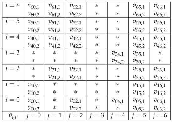
is a vector in ${\mathbb{F}}^{\frac{(\gamma +1)(\gamma +2)}{2}n}$, and $\mathbf{H}$ is a $\frac{(\gamma +\nu +1)(\gamma +\nu +2)}{2}(n-k)\times \frac{(\gamma +1)(\gamma +2)}{2}n$ matrix over $\mathbb{F}$. An example of this matrix correspondent to a parity-check matrix $\widehat{\mathbf{H}}(z_1,z_2)={\sum }_{0\le i+j\le 3}\mathbf{H}(i,j)z_1^i{z}_2^j$ is presented in Figure 1. Is easy to see that it does not follow the same pattern of construction as the partial parity-check matrix in the 1D case. Note that all the matrix coefficients $H(i,j)$ of $\widehat{\mathbf{H}}(z_1,z_2)$ appeared in all the columns following the previously established order ≺ with the particularity that, for $t=0,1,2,\dots$ in the block columns with indices $\frac{t(t+1)}{2}+1,\frac{t(t+1)}{2}+2,\dots ,\frac{t(t+1)}{2}+t+1$, the coefficients $H(i,j)$ with $i+j=d$ for $d=0,1,2,\dots ,\delta -1$ were separated from the matrices $H(i,j)$ with $i+j=d+1$ by t zero blocks.

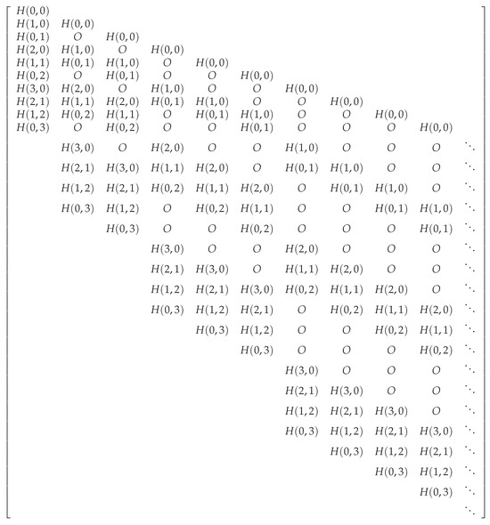
Figure 1. Matrix H.

Consider now that $\widehat{\mathbf{v}}(z_1,z_2)\in \mathbb{F}[z_1,z_2]$ has been transmitted over an erasure channel. We define the support of $\widehat{\mathbf{v}}(z_1,z_2)={\sum }_{(a,b)\in {\mathbb{N}}_0^2}v(a,b)z_1^a{z}_2^b$ as the set of indices of the coefficients of $\widehat{\mathbf{v}}(z_1,z_2)$ that are non-zero, i.e.,

$$\mathrm{supp}\left(\widehat{\mathbf{v}}(z_1,z_2)\right)=\{(a,b)\in {\mathbb{N}}_0^2:v(a,b)\ne 0\}.$$

Let $\mathcal{E}\left(\widehat{\mathbf{v}}(z_1,z_2)\right)$ be the set of indices of the support of $\widehat{\mathbf{v}}(z_1,z_2)$ in which there are erasures in the corresponding coefficients of $\widehat{\mathbf{v}}(z_1,z_2)$ and $\overline{\mathcal{E}}\left(\widehat{\mathbf{v}}(z_1,z_2)\right)=\mathrm{supp}\left(\widehat{\mathbf{v}}(z_1,z_2)\right)\backslash \mathcal{E}\left(\widehat{\mathbf{v}}(z_1,z_2)\right)$, i.e., the set of indices of the support of $\widehat{\mathbf{v}}(z_1,z_2)$ correspond to the coefficients that were correctly received. For the sake of simplicity, and if the context allows it, we will denote $\mathcal{E}\left(\widehat{\mathbf{v}}(z_1,z_2)\right)$ as $\mathcal{E}$. In Figure 2 an example of erasures distributed in the plane is presented.

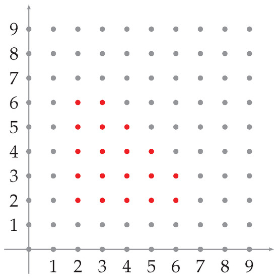
Figure 2. Erasures (red dots) distributed in ${\mathbb{N}}^2$.

Since we have the kernel representation (4) of the code in a block fashion, we can consider the equivalent linear system ${\mathbf{H}}_{\mathcal{E}}{\mathbf{v}}_{\mathcal{E}}=-{\mathbf{H}}_{\overline{\mathcal{E}}}{\mathbf{v}}_{\overline{\mathcal{E}}}$, where ${\mathbf{H}}_{\mathcal{E}}$ and ${\mathbf{H}}_{\overline{\mathcal{E}}}$ denote the submatrices of $\mathbf{H}$ where block columns are indexed by $\mathcal{E}$ and $\overline{\mathcal{E}}$, respectively. Correspondingly, ${\mathbf{v}}_{\mathcal{E}}$ and ${\mathbf{v}}_{\overline{\mathcal{E}}}$ refer to the subvectors of $\mathbf{v}$, whose block rows are indexed by $\mathcal{E}$ and $\overline{\mathcal{E}}$, respectively. In order to recover the erasures, we solved the linear system ${\mathbf{H}}_{\mathcal{E}}{\mathbf{v}}_{\mathcal{E}}=-{\mathbf{H}}_{\overline{\mathcal{E}}}{\mathbf{v}}_{\overline{\mathcal{E}}}$ by considering the erased components of ${\mathbf{v}}_{\mathcal{E}}$ as the unknowns. Note that ${\mathbf{H}}_{\overline{\mathcal{E}}}{\mathbf{v}}_{\overline{\mathcal{E}}}$ is known.

As pointed out in [9], this system is massive even when the parameters of the code are small. The authors in this paper developed an algorithm to deal with this situation in being able to recover the information more efficiently. They proposed to decode it by a set of lines, that is, to choose a set of erasures in a line ${\mathcal{E}}^l$ (i.e., horizontal (${\mathcal{E}}^h$), vertical (${\mathcal{E}}^v$), or diagonal (${\mathcal{E}}^d$)), as well as to define a neighborhood for this set of erasures and then use all the correct information within these related coefficients to construct and solve a linear system.

Next, we describe such a method for the correction of erasures in horizontal lines, wherein the method for vertical and diagonal will be analogous. Let us consider a subset of $\mathcal{E}$, ${\mathcal{E}}_s^h$, where its subindices lie in an horizontal line with the vertical coordinate s, that is,

$${\mathcal{E}}_s^h=\{(r,s)r\in {\mathbb{N}}_0\}\cap \mathcal{E}.$$

(5)

With this in mind we can “rewrite” (4) as

$${\mathbf{H}}_{{\mathcal{E}}^h}{\mathbf{v}}_{{\mathcal{E}}^h}=-{\mathbf{H}}_{\overline{{\mathcal{E}}^h}}{\mathbf{v}}_{\overline{{\mathcal{E}}^h}},$$

(6)

where—similar to the above—${\mathbf{H}}_{{\mathcal{E}}^h}$ and ${\mathbf{H}}_{\overline{{\mathcal{E}}^h}}$ indicate the submatrices of $\mathbf{H}$ that are indexed by ${\mathcal{E}}^h$ and $\overline{{\mathcal{E}}^h}=supp\left(\widehat{\mathbf{v}}(z_1,z_2)\right)\backslash {\mathcal{E}}^h$ block-wise, respectively, as well as where ${\mathbf{v}}_{{\mathcal{E}}^h}$ and ${\mathbf{v}}_{\overline{{\mathcal{E}}^h}}$ are defined analogously. (Note that ${\mathbf{v}}_{\overline{{\mathcal{E}}^h}}$ may contain erasures.)

Definition 8. 

Let $W_t$ be a horizontal window of length $t+1$. i.e.,

$$W_t=\{(r,s),(r+1,s),\dots ,(r+t,s)\},$$

for some $r\in {\mathbb{N}}_0$. We then define the following neighborhood of $W_t$ as

$$\begin{array}{ccc}{\mathrm{\Omega }}_{\nu }\left(W_t\right)& =& \left\{(a,b)|r-\nu \le a\le r+t+\nu ,s-\nu \le b\le s,\right.\\ & & \left.a+b\ge r+s-\nu ,r\ge \nu ,s\ge \nu \right\}\end{array}.$$

Example 3. 

Let $W_3=\{(3,4),(4,4),(5,4),(6,4)\}$, which is represented in Figure 3 as big red dots. In addition, ${\mathrm{\Omega }}_2\left(W_3\right)$ is depicted in Figure 3.

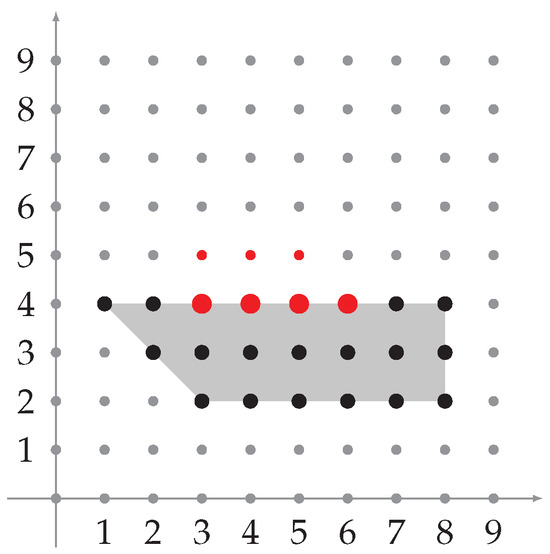
Figure 3. ${\mathrm{\Omega }}_2\left(W_3\right)$, neighborhood of $W_3$.

Note that the neighborhood is constituted of an aligned set of triangles. The main role of the above defined neighbors in the decoding process is described in the next set of results from [9].

Lemma 2 

([9]). Let $\mathcal{C}=Ke{r}_{\mathbb{F}[z_1,z_2]}\widehat{H}(z_1,z_2)$ with $\widehat{H}(z_1,z_2)={\sum }_{0\le i+j\le \nu }H(i,j)z_1^i{z}_2^j$. Suppose that $\widehat{\mathbf{v}}(z_1,z_2)\in \mathcal{C}$ is a transmitted codeword, then $\mathcal{E}$ is the support of its coefficients with erasures and ${\mathcal{E}}^h\subseteq \mathcal{E}$ is the support of the coefficients with erasures that are distributed on a horizontal line in ${\mathbb{N}}_0^2$ in a window W of length $t+1$ such that ${\mathcal{E}}^h\subset W$. Consider $\mathbf{H}$ and $\mathbf{v}$ as in (4), as well as ${\mathbf{H}}_W$ and ${\mathbf{v}}_W$ as in (6). Then, define the vector ${\mathbf{v}}_{\mathrm{\Omega }}$ by selecting the coefficients $v(c,d)$ of $\mathbf{v}$ with $(c,d)\in {\mathrm{\Omega }}_{\nu }\left(W\right)\backslash W$. Define ${\mathbf{H}}_{{\mathrm{\Omega }}_{\nu }}$ as a submatrix of $\mathbf{H}$ accordingly. Then, it holds that

$${\mathbf{H}}_W{\mathbf{v}}_W=-{\mathbf{H}}_{{\mathrm{\Omega }}_{\nu }}{\mathbf{v}}_{{\mathrm{\Omega }}_{\nu }},$$

(7)

where

$${\mathbf{H}}_W=\left[\begin{array}{ccccccc}H(0,0)& & & & & & \\ H(1,0)& H(0,0)& & & & & \\ H(2,0)& H(1,0)& H(0,0)& & & & \\ ⋮& ⋮& ⋮& \ddots & & & \\ H(\nu ,0)& H(\nu -1,0)& H(\nu -2,0)& & & & \\ & H(\nu ,0)& H(\nu -1,0)& \cdots & \cdots & H(0,0)& \\ & \ddots & & \ddots & & \ddots & \\ & & \ddots & & \ddots & & H(0,0)\\ & & & & \ddots & & ⋮\\ & & & & & H(\nu ,0)& H(\nu -1,0)\\ & & & & & & H(\nu ,0)\end{array}\right],$$

(8)

is an $(n-k)(t+1+\nu -j)\times n(t+1)$ matrix.

It is easy to see that the structure of the matrix in (8) is the same as the partial parity-check matrix of a 1D convolutional code. By taking into account this similarity we define the 1D convolutional code ${\mathcal{C}}^h$, which is associated with a 2D convolutional code $\mathcal{C}$ as follows:

$${\mathcal{C}}^h=Ke{r}_{\mathbb{F}\left[z\right]}{\widehat{H}}^{\left(h\right)}\left(z\right),$$

(9)

where

$${\widehat{H}}^{\left(h\right)}\left(z\right)=H(0,0)+H(1,0)z+\cdots +H(\nu ,0)z^{\nu }$$

(10)

with column distances $d_j^c(\ell )$, $\ell \ge 0$.

Lemma 3 

([9]). Let $\mathcal{C}=Ke{r}_{\mathbb{F}[z_1,z_2]}\widehat{H}(z_1,z_2)$ with $\widehat{H}(z_1,z_2)={\sum }_{0\le i+j\le \nu }H(i,j)z_1^i{z}_2^j$. Suppose that $\widehat{\mathbf{v}}(z_1,z_2)\in \mathcal{C}$ is a transmitted codeword, $\mathcal{E}$ is the support of its coefficients with erasures, and ${\mathcal{E}}^h\subseteq \mathcal{E}$ is the support of the coefficients with its erasures distributed on a horizontal line in ${\mathbb{N}}_0^2$ in a window W of length $t+1$ such that ${\mathcal{E}}^h\subset W$. If ${\mathrm{\Omega }}_{\nu }\left(W_t\right)$ contains only indices in ${\mathcal{E}}^h$ (and not in $\mathcal{E}\backslash \left({\mathcal{E}}^h\right)$), we have

$${\mathbf{H}}_W{\mathbf{v}}_W={\mathbf{a}}_{j_0},$$

(11)

where ${\mathbf{a}}_{j_0}=-{\mathbf{H}}_{{\mathrm{\Omega }}_{\nu }}{\mathbf{v}}_{{\mathrm{\Omega }}_{\nu }}$ is known and ${\mathbf{H}}_W$ is as in (8). Moreover, consider the 1D convolutional code ${\mathcal{C}}_h$ with a parity check as defined in (10) and with a column distance $d_{\ell },\ell \ge 0$. If there exists ${\ell }_0$ such that at most there are $d_{{\ell }_0}^c-1$ erasures that occur in any $({\ell }_0+1)n$ consecutive components of ${\mathbf{v}}_W$, then we can completely recover the vector ${\mathbf{v}}_W$.

The requirement for ${\mathrm{\Omega }}_W$ to contain just the erasures in ${\mathcal{E}}^h$ plays the role of the safe space for the 1D convolutional codes.

Example 4. 

Let $\mathcal{C}$ be a 2D convolutional code with a parity-check matrix as follows:

$$\widehat{H}(z_1,z_2)=H(0,0)+H(1,0)z_1+H(0,1)z_2+H(2,0)z^2+H(1,1)z_1{z}_2+H(0,2)z_2^2.$$

We define the 1D convolutional codes ${\mathcal{C}}^h=Ke{r}_{\mathbb{F}\left[z\right]}{\widehat{H}}^{\left(0\right)}$, where

$${\widehat{H}}^{\left(0\right)}=H(0,0)+H(1,0)z+H(2,0)z^2.$$

Let us assume that we receive the pattern of erasures that are shown in Figure 4 (red dots), and let us consider the erasures on the first line (big red dots), i.e.,

$${\mathcal{E}}_3^h=\{v(3,3),v(4,3),v(5,3)\}$$

and set $W={\mathcal{E}}_3^h$. To correct ${\mathcal{E}}_3^h$, we use the code $\mathcal{C}$ by Lemma 3. To do so, we build a system as in (3), where

$${\mathbf{H}}_{{\mathcal{E}}^h}^0=\left[\begin{array}{cccc}H(0,0)& & & \\ H(1,0)& H(0,0)& & \\ H(2,0)& H(1,0)& H(0,0)& \\ & H(2,0)& H(1,0)& H(0,0)\\ & & H(2,0)& H(1,0)\\ & & & H(2,0)\end{array}\right];{\mathbf{v}}_{{\mathcal{E}}^h}=\left[\begin{array}{c}v(3,4)\\ v(4,4)\\ v(5,4)\\ v(6,4)\end{array}\right]$$

and

$${\mathbf{a}}_0=-\left[\begin{array}{cccccccccccccc}H(0,2)& H(1,1)& H(2,0)& \mathbf{0}& H(0,1)& H(1,0)& & & & & & & & \\ & & & H(0,2)& H(1,1)& H(2,0)& \mathbf{0}& H(0,1)& & & & & & \\ & & & & & & H(0,2)& H(1,1)& \mathbf{0}& H(0,1)& & & & \\ & & & & & & & & H(0,2)& H(1,1)& \mathbf{0}& H(0,1)& & \\ & & & & & & & & & & H(0,2)& H(1,1)& \mathbf{0}& H(0,1)\\ & & & & & & & & & & & & H(0,2)& H(1,1)\end{array}\right]\left[\begin{array}{c}v(3,2)\\ v(2,3)\\ v(1,4)\\ v(4,2)\\ v(3,3)\\ v(2,4)\\ v(5,2)\\ v(4,3)\\ v(6,2)\\ v(5,3)\\ v(7,2)\\ v(6,3)\\ v(8,2)\\ v(7,3)\end{array}\right]$$

Figure 4. Erasures (red dots) distributed in ${\mathbb{N}}^2$.

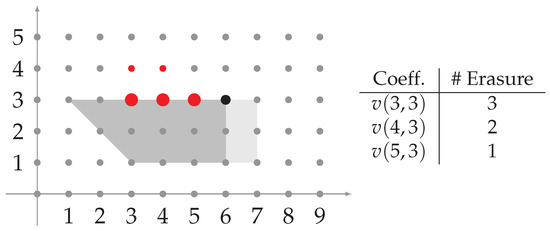
In Lemma 3, it is said that one can conduct a partial correction in line by using the column distances of the used convolutional code. In Example 5, we can see how this partial recovery is performed.

Example 5. 

Let $\mathcal{C}$ be a $(3,1,2)$ 2D convolutional code with a parity-check matrix $H(z_1,z_2)=H(0,0)+H(1,0)z_1+H(0,1)z_2+H(2,0)z_1^2+H(1,1)z_1{z}_2+H(0,2)z_2^2$. Let us assume that we receive the pattern of erasures that are shown in Figure 4 (red dots). As mentioned above, we will try to recover the horizontal lines from below to above; therefore, we will try to recover the erasures on the first line (big red dots), i.e., ${\mathcal{E}}^h=\{v(3,3),v(4,3),v(5,3)\}$. Since we have some erasures on the top line, we will consider the code ${\mathcal{C}}^h$ associated with the neighbor ${\mathrm{\Omega }}_2\left({\mathcal{E}}^h\right)$ (i.e., the whole gray area).

We assumed that the 1D convolutional code ${\mathcal{C}}_0$ has the column distances $d_0=2$, $d_1=4$, $d_2=5$, and $d_3=6$. Note that the total amount of erasures holds that $6\le d_3-1=6$; therefore, we have to consider a window of a $(L+1)n=(3+1)3=12$ size (the big red dots and black dot). By following the proof of Lemma 3 in [9], we picked the first $(L+1)(n-k)=32$ equations from the system ${\tilde{\mathbf{H}}}_{{\mathcal{E}}^h}^0{\tilde{\mathbf{v}}}_{{\mathcal{E}}^h}={\tilde{a}}_0$ and obtained the following system:

$$\left[\begin{array}{cccc}H(0,0)& & & \\ H(1,0)& H(0,0)& & \\ H(2,0)& H(1,0)& H(0,0)& \\ & H(2,0)& H(1,0)& H(0,0)\end{array}\right]\left[\begin{array}{c}v(3,3)\\ v(4,3)\\ v(5,3)\\ v(6,3)\end{array}\right]={\tilde{\mathbf{a}}}_0.$$

As proven in [13], once we solved this system we were able to successfully recover the erasures in $v(3,3)$. We then shifted the window and repeated the process until the recovery was fully completed.

As we mentioned at the beginning of this section, analogous methods can be described by taking lines of erasures in a vertical or diagonal fashion. In [9], it was said that, to decode a set of erasures in the grid ${\mathbb{N}}^2$, one can carry out the horizontal decoding as was explicitly conducted above in the “from below to above” direction until is not possible to correct anymore. Afterward, execute the algorithm by taking the vertical lines of the erasures and correcting them in the “from left to right” direction until no more corrections can be made. Finally, we followed the same procedure with diagonal lines of erasures, and we then repeated this cycle until any of them were able to recover further information.

3. Construction of 2D Convolutional Codes from 1D Convolutional Codes

In this section, we propose a construction of 2D convolutional codes from a 1D convolutional code.

Let $\widehat{\mathcal{C}}$ be an $(n,k)$ non-catastrophic 1D convolutional code with a parity-check matrix $\widehat{H}\left(z\right)={\sum }_{i=0}^{2\nu }{H}_i{z}^i\in {\mathbb{F}}_q{\left[z\right]}^{(n-k)\times n}$. Consider the 2D convolutional code $\mathcal{C}$, which is defined by the parity-check matrix

$$\begin{array}{l}H(z_1,z_2)={\displaystyle \sum _{i=0}^{\nu }}{\displaystyle \sum _{j=i}^{2i}}{H}_j{z}_1^{2i-j}{z}_2^{j-i}\\ \hspace{1em}\hspace{1em}\hspace{1em}\hspace{1em}\hspace{1em}\hspace{1em}\hspace{1em}\hspace{1em}\hspace{1em}\hspace{1em}=H_0+H_1{z}_1+H_2{z}_2+H_2{z}_1^2+H_3{z}_1{z}_2\\ \hspace{1em}\hspace{1em}\hspace{1em}\hspace{1em}\hspace{1em}\hspace{1em}\hspace{1em}\hspace{1em}\hspace{1em}\hspace{1em}\hspace{1em}\hspace{1em}\hspace{1em}\hspace{1em}\hspace{1em}\hspace{1em}\hspace{1em}\hspace{1em}\hspace{1em}\hspace{1em}+H_4{z}_2^2+\cdots +H_{\nu }{z}_1^{\nu }+\cdots +H_{2\nu }{z}_2^{\nu }.\end{array}$$

(12)

We consider the 1D convolutional codes associated with $\mathcal{C}$ (named horizontal, vertical, and diagonal), which are constructed by its line positions as follows:

• Horizontal: ${\mathcal{C}}^h=Ker{H}^h\left(z\right)$;
• Vertical: ${\mathcal{C}}^v=Ker{H}^v\left(z\right)$;
• Diagonal: ${\mathcal{C}}^d=Ker{H}^d\left(z\right)$,

where the matrices $H^h,H^v,$and$H^d\in {\mathbb{F}}_q{\left[z\right]}^{(n-k)\times n}$ are defined by

$$\begin{array}{cc}\hfill H^h\left(z\right)& =\sum _{i=0}^{\nu }{H}_i{z}^i\hfill \\ \hfill & =H_0+H_{1}z+H_2{z}^2+\cdots +H_{\nu }{z}^{\nu }.\hfill \\ \hfill H^v\left(z\right)& =\sum _{i=0}^{\nu }{H}_{2i}{z}^i\hfill \\ \hfill & =H_0+H_{2}z+H_4{z}^2+\cdots +H_{2\nu }{z}^{\nu }.\hfill \\ \hfill H^d\left(z\right)& =\sum _{i=0}^{\nu }{H}_{\nu +i}{z}^i\hfill \\ \hfill & =H_{\nu }+H_{\nu +1}z+H_{\nu +2}{z}^2+\cdots +H_{2\nu }{z}^{\nu }.\hfill \end{array}$$

Naturally, at this point, one wants to know if the optimal properties of $\widehat{\mathcal{C}}$ are inherited by the line associated codes ${\mathcal{C}}^h$, ${\mathcal{C}}^v$, and ${\mathcal{C}}^d$. In particular, we were interested in the complete-MDP property. In general, these codes did not inherit this property as the next examples show.

Example 6. 

In [28], Almeida and Lieb presented a description of all $(2,1,2)$ complete-MDP convolutional codes over the smallest possible fields. Let $\widehat{\mathcal{C}}$ be the one of these $(2,1,2)$ convolutional code over ${\mathbb{F}}_{13}$, which is defined by the parity-check matrix $\widehat{H}\left(z\right)=H_o+H_{1}z+H_2{z}^2$, where $H_2=[1,1],H_1=[2,9] and H_0=[8,8]$, which is a complete-MDP (as stated in Theorem 13 [28]). Note that the partial parity-check matrices for the vertical, horizontal, and diagonal associated codes are

$${\mathfrak{H}}^v=\left(\begin{array}{cccc}{H}_2& H_0& & \\ & H_2& H_0& \\ & & H_2& H_0\end{array}\right){\mathfrak{H}}^h=\left(\begin{array}{cccc}{H}_1& H_0& & \\ & H_1& H_0& \\ & & H_1& H_0\end{array}\right){\mathfrak{H}}^d=\left(\begin{array}{cccc}{H}_2& H_1& & \\ & H_2& H_1& \\ & & H_2& H_1\end{array}\right),$$

respectively, and the parameters of these codes are $(2,1,1)$. For ${\mathfrak{H}}^v$, the non-trivial zero minor, which is zero, can be obtained by considering columns 1, 5, and 6:

$$\left|\begin{array}{ccc}1& 0& 0\\ 0& 8& 8\\ 0& 1& 1\end{array}\right|,$$

which means that ${\mathcal{C}}^v$ is not a complete-MDP. With a similar reasoning, we see that ${\mathcal{C}}^h$ and ${\mathcal{C}}^d$ are also not complete-MDPs. As such, in this case, no associated code maintained the complete-MDP property.

Next, we considered a 1D complete-MDP, which is defined in [17], as follows:

Lemma 4 

([17]). For $a,b\in \mathbb{N}$, with $b<a$, let

$$X=\left[\begin{array}{cccc}1& & & 0\\ 1& \ddots & & \\ & \ddots & \ddots & \\ 0& & 1& 1\end{array}\right]\in {\mathbb{Z}}^{a\times a}$$

and let $\widehat{X}:={\left(X^b\right)}_{i_1,...,i_r}^{j_1,...,j_r}$ be constructed out of rows $1\le i_1\le \cdots i_r\le a$ and columns $1\le j_1\le \cdots \le j_r\le a$ of

$$X^b=\left[\begin{array}{ccccccc}1& & & & & & 0\\ \left(\genfrac{}{}{0pt}{}{b}{1}\right)& \ddots & & & & & \\ ⋮& \ddots & \ddots & & & & \\ \left(\genfrac{}{}{0pt}{}{b}{b-1}\right)& & \ddots & \ddots & & & \\ 1& \ddots & & \ddots & \ddots & & \\ & \ddots & \ddots & & \ddots & \ddots & \\ 0& & 1& \left(\genfrac{}{}{0pt}{}{b}{b-1}\right)& \cdots & \left(\genfrac{}{}{0pt}{}{b}{1}\right)& 1\end{array}\right].$$

Then, we have $det\left(\widehat{X}\right)\ge 0$ and $det\left(\widehat{X}\right)>0\iff j_l\in \{i_l-b,\dots ,i_l\}$ for $l=1,\dots ,r.$

Theorem 5 

([17]). With the notation from the preceding lemma, choose $X\in {\mathbb{F}}^{(\nu +L+1)n\times (\nu +L+1)n},$ i.e., $a:=(\nu +L+1)n,$ as well as $b:=\nu n+k.$

For $j=0,...,L$, set $I_j=\{(\nu +j)n+k+1,...,(\nu +j+1)n\}$ and $I={\cup }_{j=0}^L{I}_j.$ Then, those rows of $X^b$, whose indices lie in I, form the partial parity-check matrix of an ($n,k,\delta$) complete-MDP convolutional code if the characteristic of the field is greater than ${\left(\genfrac{}{}{0pt}{}{\nu n+k}{\lfloor 1/2(\nu n+k)\rfloor }\right)}^{(n-k)(L+1)}·{\left((n-k)(L+1)\right)}^{1/2(n-k)(L+1)}.$

Let $\widehat{\mathcal{C}}$ be the 1D complete-MDP convolutional code defined in Theorem 5 with the degree $2\delta$. In the construction, it was assumed that $2\delta =2\nu (n-k).$ The associated line codes defined from $\widehat{\mathcal{C}}$ had the parameters $(n,k,\delta )$.

The next theorem shows that the associated vertical 1D convolutional code was also a complete-MDP.

Theorem 6. 

Let $\mathcal{C}$ be a 2D convolutional code that was constructed as in (12) by using a $(n,k,2\delta )$ 1D complete-MDP convolutional code $\widehat{\mathcal{C}}$, as shown in Theorem 5 with the parity-check matrix $H\left(z\right)={\sum }_{i=0}^{2\nu }{H}_i{z}^i$, where $2\nu =\frac{2\delta }{n-k}$. Then, the associated line code ${\mathcal{C}}^v$ with the parity-check matrix

$$\begin{array}{cc}\hfill H^v\left(z\right)& =\sum _{i=0}^{\nu }{H}_{2i}{z}^i\hfill \end{array}$$

is an $(n,k,\delta )$ 1D complete-MDP convolutional code.

Proof. 

The proof follows since every full-size minor of ${\mathfrak{H}}^v$ that is not trivially zero is a non-trivial minor of $X^b$, which is a super-regular matrix by Lemma 4. In fact, Lieb showed Theorem 5 [17]. This proof involves demonstrating that the conditions of the indices of the columns in the partial parity-check matrix $\mathfrak{H}$, which describes non-trivial zero full-size minors, are equivalent to the conditions outlined in Lemma 4. Moreover, both sets of conditions were found to be mutually equivalent to $j_l\in \{l+kx,\dots ,l+kx+\nu n+k\},$ where $x\in \{0,\dots ,L\}$ is chosen such that $l\in \left\{x\right(n-k)+1,\dots ,(x+1\left)\right(n-k\left)\right\}.$ Now, to prove the theorem, it is sufficient to observe that the columns of ${\mathfrak{H}}^v$ still satisfy $j_l\in \{l+2kx,\dots ,l+2kx+2\nu n+k\}\backslash \{(x+1)n+1,\dots (x+2)n\},$ where $x\in \{0,\dots ,L/2\}$ is chosen such that $l\in \left\{2x\right(n-k)+1,\dots ,(2x+1\left)\right(n-k\left)\right\}.$ It is worth remembering that ${\mathfrak{H}}^v$ is obtained from $\mathfrak{H}$ by removing all the block-rows (of size $n-k$) and block-columns (of size n) with odd indices. □

Although the horizontal and diagonal associated line codes do not maintain the optimality as is the case in the vertical one, these codes still satisfy a weaker optimality property.

Theorem 7. 

Let $\mathcal{C}$ be a 2D convolutional code, constructed as in (12), by using a $(n,k,2\delta )$ 1D complete-MDP convolutional code $\widehat{\mathcal{C}}$, as represented in Theorem 5 with the parity-check matrix $H\left(z\right)={\sum }_{i=0}^{2\nu }{H}_i{z}^i$, where $2\nu =\frac{2\delta }{n-k}$. Then, the horizontal ${\mathcal{C}}^h$ and the reverse diagonal $\overline{{\mathcal{C}}^d}$ associated line codes are expressed with the parity-check matrices

$$\begin{array}{cc}\hfill H^h\left(z\right)& =\sum _{i=0}^{\nu }{H}_i{z}^i\hfill \\ \hfill & =H_0+H_{1}z+H_2{z}^2+\cdots +H_{\nu }{z}^{\nu }.\hfill \\ \hfill \overline{H^d}\left(z\right)& =\sum _{i=0}^{\nu }{H}_{2\nu -i}{z}^i\hfill \\ \hfill & =H_{\nu }+H_{\nu +1}z+H_{\nu +2}{z}^2+\cdots +H_{2\nu }{z}^{\nu }.\hfill \end{array}$$

respectively, which are $(n,k,\delta )$ 1D convolutional codes with the column distance $d_{\nu }^c=(n-k)(\nu +1)+1.$

Proof. 

By ([15], Prop 2.1), we need to show that the matrices

$${\mathcal{H}}^h≔\left[\begin{array}{cc}{H}_0& \\ ⋮& \ddots & \\ H_{\nu }& \cdots & H_0\end{array}\right]\overline{{\mathcal{H}}^d}≔\left[\begin{array}{cc}{H}_{2\nu }& \\ ⋮& \ddots & \\ H_{\nu }& \cdots & H_{2\nu }\end{array}\right]$$

have the property that every full-size minor that is non-trivially zero is non-zero. Note that $\overline{{\mathcal{H}}^d}$ can be viewed as the submatrix of the partial parity-check matrix of $\widehat{\mathcal{C}}$, $\mathfrak{H}$ by considering it as the first $(\nu +1)(n-k)$ rows and $(\nu +1)n$ columns. In this context, considering that $\mathfrak{H}$ is superregular, we can deduce that, within $\overline{{\mathcal{H}}^d}$, every non-trivial full-size minor is non-zero.

For ${\mathcal{H}}^h$, note that it is exactly the submatrix of $\mathfrak{H}$ that considers the first $(\nu +1)(n-k)$ rows and the columns with indices in the set $\{2\nu n+1,\dots ,(3\nu +1)n+1\}$, as well as the conditions over the columns of the nontrivial minors that imply the condition of Lemma 4. □

While it is demonstrated in this section that the associated line 1D convolutional codes do not necessarily inherit the complete-MDP property of the 1D convolutional code $\widehat{\mathcal{C}}$, there exist codes in which this phenomenon occurs. The next section presents a construction of a 2D convolutional code from a complete-MDP 1D convolutional code, whose associated line of 1D convolutional codes are also complete-MDPs. These types of codes are the ones that perform better with the decoding procedure that we are considering, which we will also see later in Section 5.

4. An Optimal Construction

In this section, we present the construction of an optimal 2D convolutional code in the sense that all its associated line codes hold the complete-MDP property. In this case, we will use a complete-MDP 1D convolutional code that was introduced in [17].

Theorem 8 

([17]). Let $n,k,\delta \in \mathbb{N}$ with $k<n$ and $(n-k)|\delta$, and let α be a primitive element of a finite field ${\mathbb{F}}_{p^N}$ with $N>(L+1)2^{(\nu +2)n-k-1}$. Then, $H\left(z\right)={\sum }_{i=0}^{\nu }{H}_i{z}^i$ with

$$H_i=\left[\begin{array}{ccc}{\alpha }^{2^{in}}& \cdots & {\alpha }^{2^{(i+1)n}-1}\\ ⋮& & ⋮\\ {\alpha }^{2^{(i+1)n-k-1}}& \cdots & {\alpha }^{2^{(i+2)n}-k-2}\end{array}\right]$$

for $i=0,\dots ,\nu =\frac{\delta }{n-k}$ is the parity-check matrix of an $(n,k,\delta )$ complete-MDP convolutional code.

In order to prove the optimality of our constructions, we will need the next result, which states that the matrices considered in Theorem 8 are superregular.

Proposition 2 

([16]). Let α be a primitive element of a finite field $\mathbb{F}={\mathbb{F}}_{p^N}$, and let $B=\left[b_{i\ell }\right]$ be a matrix over $\mathbb{F}$ with the following properties:

1. 

If $b_{i\ell }\ne 0$, then $b_{i\ell }={\alpha }^{{\beta }_{i\ell }}$ for a positive integer ${\beta }_{i\ell }$;

2. 

If $b_{i\ell }=0$, then $b_{i^{\prime }\ell }=0$ for any $i^{\prime }>i$, or $b_{i{\ell }^{\prime }}=0$ for any ${\ell }^{\prime }<\ell$;

3. 

If $\ell <{\ell }^{\prime }$, $b_{i\ell }\ne 0$, and $b_{i{\ell }^{\prime }}\ne 0$, then $2{\beta }_{i\ell }\le {\beta }_{i{\ell }^{\prime }}$;

4. 

If $i<i^{\prime }$, $b_{i\ell }\ne 0$, and $b_{i^{\prime }\ell }\ne 0$, then $2{\beta }_{i\ell }\le {\beta }_{i^{\prime }\ell }$.

Suppose N is greater than any exponent of α appearing as a non-trivial term of any minor of B, then B is superregular.

It is worth mentioning that if we have two matrices A and B that are equivalent (i.e., that we can obtain A from B by using row and column linear transformations), and if one of them holds the hypothesis of the theorem, then both of them are superregular.

Theorem 9. 

Let $\mathcal{C}$ be a 2D convolutional code, which was constructed as in (12) by using a $(n,k,2\delta )$ 1D complete-MDP convolutional code $\widehat{\mathcal{C}}$, as expressed in Theorem 8, with the parity-check matrix $H\left(z\right)={\sum }_{i=0}^{2\nu }{H}_i{z}^i$, where $\nu =\frac{\delta }{n-k}$. Then, the associated line codes, ${\mathcal{C}}^h$, ${\mathcal{C}}^v$, and ${\mathcal{C}}^d$ are $(n,k,\delta )$ 1D complete-MDP convolutional codes.

Proof. 

Recall that the associated line 1D convolutional codes ${\mathcal{C}}^h$, ${\mathcal{C}}^v$, and ${\mathcal{C}}^d$ have the parity-check matrices

$$\begin{array}{cc}\hfill H^h\left(z\right)& =\sum _{i=0}^{\nu }{H}_i{z}^i\hfill \\ \hfill & =H_0+H_{1}z+H_2{z}^2+\cdots +H_{\nu }{z}^{\nu }.\hfill \\ \hfill H^v\left(z\right)& =\sum _{i=0}^{\nu }{H}_{2i}{z}^i\hfill \\ \hfill & =H_0+H_{2}z+H_4{z}^2+\cdots +H_{2\nu }{z}^{\nu }.\hfill \\ \hfill H^d\left(z\right)& =\sum _{i=0}^{\nu }{H}_{\nu +i}{z}^i\hfill \\ \hfill & =H_{\nu }+H_{\nu +1}z+H_{\nu +2}{z}^2+\cdots +H_{2\nu }{z}^{\nu }.\hfill \end{array}$$

To see that ${\mathcal{C}}^h$, ${\mathcal{C}}^v$, and ${\mathcal{C}}^d$ are 1D complete-MDP codes, we need to prove that the non-trivial zero full-size minors of the matrices

$$\begin{array}{c}{\mathfrak{H}}^h=\left[\begin{array}{ccccccc}{H}_{\nu }& H_{\nu -1}& \dots & H_0& & & \\ & H_{\nu }& & H_1& H_0& & \\ & & \ddots & & \ddots & \ddots & \\ & & & H_{\nu }& \dots & H_1& H_0\end{array}\right]\in {\mathbb{F}}^{(L^{\prime }+1)(n-k)\times (\nu +L^{\prime }+1)n},\hfill \\ {\mathfrak{H}}^v=\left[\begin{array}{ccccccc}{H}_{2\nu }& H_{2\nu -2}& \dots & H_0& & & \\ & H_{2\nu }& & H_2& H_0& & \\ & & \ddots & & \ddots & \ddots & \\ & & & H_{2\nu }& \dots & H_2& H_0\end{array}\right]\in {\mathbb{F}}^{(L^{\prime }+1)(n-k)\times (\nu +L^{\prime }+1)n},\\ \hfill {\mathfrak{H}}^d=\left[\begin{array}{ccccccc}{H}_{2\nu }& H_{\nu -1}& \dots & H_{\nu }& & & \\ & H_{2\nu }& & H_{\nu +1}& H_{\nu }& & \\ & & \ddots & & \ddots & \ddots & \\ & & & H_{2\nu }& \dots & H_{\nu +1}& H_{\nu }\end{array}\right]\in {\mathbb{F}}^{(L^{\prime }+1)(n-k)\times (\nu +L^{\prime }+1)n}.\end{array}$$

(13)

are non-zero, where $L^{\prime }=\frac{L}{2}$. To this end, we will see that they satisfy the conditions of Proposition 2, i.e., that they are superregular.

First, since $\widehat{\mathcal{C}}$ is a complete-MDP code, we have

$$\mathfrak{H}=\left[\begin{array}{ccccccc}{H}_{2\nu }& H_{\nu -1}& \dots & H_0& & & \\ & H_{2\nu }& & H_1& H_0& & \\ & & \ddots & & \ddots & \ddots & \\ & & & H_{2\nu }& \dots & H_1& H_0\end{array}\right],$$

which has the property that all its full-size minors that are not trivially zero are non-zero. Note that we can see ${\mathfrak{H}}^{\mathfrak{v}}$ as a submatrix of $\mathfrak{H}$ when removing all the block-rows and block-columns with odd indices. Now, is easy to see that if all of the non-trivial zero full-size minors of ${\mathfrak{H}}^v$ are not trivially minors of $\mathfrak{H}$, then they are non-zero.

Finally, through following the same argument as in the proof of Theorem 8 in [17], if we permute the columns of ${\mathfrak{H}}^h$ and ${\mathfrak{H}}^d$ in such a way that they have reverse order, then we have

$$\left[\begin{array}{ccccccc}& & & H_0& \dots & H_{\nu -1}& H_{\nu }\\ & & ⋰& & ⋰& ⋰& \\ & H_0& & H_{\nu -1}& H_{\nu }& & \\ H_0& H_1& \dots & H_{\nu }& & \end{array}\right]\mathrm{and}\left[\begin{array}{ccccccc}& & & H_{\nu }& \dots & H_{2\nu -1}& H_{2\nu }\\ & & ⋰& & ⋰& ⋰& \\ & H_{\nu }& & H_{2\nu -1}& H_{2\nu }& & \\ H_{\nu }& H_{\nu +1}& \dots & H_{2\nu }& & & \end{array}\right],$$

which keeps the same terms for the non-trivial zero full-size minors. It is easy to see that these matrices fulfill the conditions of Proposition 2, thus making them superregular matrices. □

Example 7. 

Consider the $(3,1,4)$ 1D convolutional code ${\mathcal{C}}^{\prime }$ over ${\mathbb{F}}_{p^N}$, which was constructed as in Theorem 8, having the parity-check matrix $H\left(z\right)=H_0+H_{1}z+H_2{z}^2$ with $H_0=\left[\begin{array}{ccc}\alpha & {\alpha }^2& {\alpha }^4\\ {\alpha }^2& {\alpha }^4& {\alpha }^8\end{array}\right]$, $H_1=\left[\begin{array}{ccc}{\alpha }^8& {\alpha }^{16}& {\alpha }^{32}\\ {\alpha }^{16}& {\alpha }^{32}& {\alpha }^{64}\end{array}\right]$, and $H_2=\left[\begin{array}{ccc}{\alpha }^{64}& {\alpha }^{128}& {\alpha }^{256}\\ {\alpha }^{128}& {\alpha }^{256}& {\alpha }^{512}\end{array}\right]$. Note that in order to obtain a complete-MDP code, $N>7168$. The 2D convolutional code obtained by following the proposed construction was a $(3,1,1)$ 2D convolutional code with the parity-check matrix

$$H(z_1,z_2)=H_0+H_1{z}_1+H_2{z}_2,$$

and its line associated codes had the following parity-check matrices:

$$\begin{array}{c}\hfill H^h\left(z\right)=H_0+H_{1}z;H^v\left(z\right)=H_0+H_{2}z;H^d\left(z\right)=H_1+H_{2}z.\end{array}$$

Note that for ${\mathcal{C}}^{\prime }$ and $L=6$, its line associated codes are therefore $L^{\prime }=3$. Now, it is clear that ${\mathfrak{H}}^v$ is a submatrix of $\mathfrak{H}$ when looking at (14); on the other hand, ${\mathfrak{H}}^h$ and ${\mathfrak{H}}^d$ cannot be seen as submatrices of $\mathfrak{H}$.

$$\mathfrak{H}=\left[\begin{array}{ccccccccc}{H}_2& H_1& H_0& & & & & & \\ & H_2& H_1& H_0& & & & & \\ & & H_2& H_1& H_0& & & & \\ & & & H_2& H_1& H_0& & & \\ & & & & H_2& H_1& H_0& & \\ & & & & & H_2& H_1& H_0& \\ & & & & & & H_2& H_1& H_0\end{array}\right];{\mathfrak{H}}^v=\left[\begin{array}{ccccc}{H}_2& H_0& & & \\ & H_2& H_0& & \\ & & H_2& H_0& \\ & & & H_2& H_0\end{array}\right].$$

(14)

5. Decoding Algorithm

In this section, we provide a decoding algorithm for the 2D convolutional codes whose associated line 1D convolutional codes were complete-MDPs. We will use Algorithm 1, which was introduced in the previous section, to perform the corrections over the lines (i.e., horizontal, vertical, and diagonal).

First, we present the construction of a sort algorithm to obtain the lines for which we will perform the correction of erasures. This procedure will provide the set of coefficients of the received codeword $v(z_1,z_2)$ for the line decoding that was presented in the previous section depending on the orientation of the line we need to correct. The mergesort$\left(\mathcal{E}\right)$ function will sort the set $\mathcal{E}\in {\mathbb{N}}^2$ by using the above order ≺.

This algorithm chooses the first horizontal line that has some erasure (i.e., the line ${\mathcal{E}}_s^h$ where s is the minimum integer such that ${\mathcal{E}}_s^h\ne \varnothing$), as well as the first vertical line that has some erasure or the last diagonal lien with erasures. By doing this, we can correct the lines as explained above. Algorithm 2 depicts the procedure explained in [9] and above in a pseudo-code fashion.

In the proposed routine, we start by extracting the coordinates with erasures $\mathcal{E}$, and we later use Algorithm 3 to obtain the sequence of vectors to be corrected by Algorithm 1. In this case, Algorithm 1 can perform analogously but by building the linear systems as in Lemma 3. After performing the decoding, depending on the amount of erasures that are recovered, it changes orientation or returns back to horizontal decoding. When it cannot correct more erasures in any orientation ($fail=3$), it stops.

Algorithm 2 Decoding 2D convolutional codes

Input:  $\mathbf{v}(z_1,z_2)$, received codeword Output:  $\mathbf{v}(z_1,z_2)$, corrected codeword   1: $fail=0$   2: $med=0$   3: $ori=0$   4: $\mathcal{E}=\left\{v(a,b)\right|v(a,b)\in \mathbf{v}(z_1,z_2)\mathrm{and}v(a,b)=0\}$   5: while  $fail<3$  do   6:      if $med=0$ then {Decides orientation depending on $med$}   7:             $ori=h$   8:             $ext=(0,L)$   9:      else if $med=1$ then 10:             $ori=v$ 11:             $ext=(L,0)$ 12:      else if $med=2$ then 13:             $ori=d$ 14:             $ext=(L,-L)$ 15:      ${\mathcal{E}}^{ori}=Algorithm2(\mathcal{E},ori)$ 16:      $e_{min}={min}_{\prec }(a,b)\in {\mathcal{E}}^{ori}$ 17:      $e_{max}={max}_{\prec }(a,b)\in {\mathcal{E}}^{ori}$ 18:      $[v_0,\dots ,v_{\ell }]≔[v\left(e_{min}\right),\dots ,v(e_{max}+ext)]$ 19:      $[v_0,\dots ,v_{\ell }]≔Algorithm1({\mathcal{C}}_{j_0},[v_0,\dots ,v_{\ell }])$ 20:      ${\mathcal{R}}^{ori}=\left\{(a,b)\right|v_i=v(a,b)\mathbf{and}{v}_i=1\}${correct coordinates} 21:      $\mathcal{E}=\mathcal{E}\backslash {\mathcal{R}}^{ori}$ 22:      if length$\left({\mathcal{R}}^{ori}\right)=\ell +1$ then {All corrected} 23:             $fail=0$ 24:             $med=0$ 25:      else if length$\left({\mathcal{R}}^{ori}\right)>\ell +1-\mathtt{length}\left({\mathcal{E}}^{ori}\right)$ then {Some corrected} 26:             $fail=0$ 27:             $med=med+1$ 28:      else if length$\left({\mathcal{R}}^{ori}\right)=\ell +1-\mathtt{length}\left({\mathcal{E}}^{ori}\right)$ then {None corrected} 29:             $fail=fail+1$ 30:             $med=med+1$

Algorithm 3 Choosing the set of coefficients ${\mathcal{E}}^i$ to be corrected

Input:  $v(z_1,z_2)$, $\mathcal{E}$ and an orientation $h,v$ or d Output:  ${\mathcal{E}}^i$ with $i\in \{h,v,d\}$.   1: if i=h then   2:    $c^h={min}_{(a,b)\in \mathcal{E}}\left\{b\right\}$                                            {We pick the index of the first row}   3:    ${\mathcal{E}}^h≔\mathtt{mergesort}\left(\left\{(a,b)\right|(a,b)\in \mathcal{E}\mathrm{and}b=c^h\}\right)$   4: else if i=v then   5:    $c^v={min}_{(a,b)\in \mathcal{E}}\left\{a\right\}$                                            {We pick the index of the first row}   6:    ${\mathcal{E}}^v≔\mathtt{mergesort}\left(\left\{(a,b)\right|(a,b)\in \mathcal{E}\mathrm{and}a=c^v\}\right)$   7: else if i=d then   8:    $c^d={max}_{(a,b)\in \mathcal{E}}\{a+b\}$                               {We pick the index of the last diagonal}   9:    ${\mathcal{E}}^d≔\mathtt{mergesort}\left(\left\{(a,b)\right|(a,b)\in \mathcal{E}\mathrm{and}a+b=c^d\}\right)$

Very recently, in [10], an alternative decoding algorithm for 2D convolutional codes was presented. The proposed method also follows the idea of decoding in two directions: horizontal and vertical. Although the main guideline is similar, the performance and the algebraic properties used are very different. Let $G(z_1,z_2)$ be the generator matrix of a 2D convolutional code, which can be expressed as follows:

$$G(z_1,z_2)=\sum _{i=0}^{{\mu }_1}{G}_i^{\left(2\right)}\left(z_2\right)z_1^i,$$

where ${\mu }_1={deg}_{z_1}\left(G(z_1,z_2)\right)$, and $G_i^{\left(2\right)}\left(z_2\right)={\sum }_i{G}_{ij}{z}_2^i$. Then, we can encode the message

$$u(z_1,z_2)=\sum _{j=0}^{m_2}{u}_j^{\left(2\right)}\left(z_2\right)z_1^j$$

to the codeword

$$v(z_1,z_2)=\sum _{j=0}^{m_2+{\mu }_2}{v}_j^{\left(2\right)}\left(z_2\right)z_1^j$$

with

$$v_j^{\left(2\right)}\left(z_2\right)=\sum _{l+k=j}{G}_l^{\left(2\right)}\left(z_2\right)u_k^{\left(2\right)}\left(z_2\right).$$

Note that, for this description, the coefficients of $v_j^{\left(2\right)}\left(z_2\right)$ form the j-th horizontal line, and the analogously coefficient $v_j^{\left(1\right)}\left(z_1\right)$ determine the j-th vertical line.

There are two main differences with respect to the algorithm described in this paper, the first of which is the decoding performance in a given line. While Algorithm 1 tries forward, backward, and complete-MDP (if possible) decoding for a given line, the method from [10] performs partial corrections that may leave gaps of erasures, whereby when it later it tries to fill those gaps it is always in the forward direction. This last-mentioned process of “filling the gaps” was performed by correcting one point at a time; however, this may make this algorithm less efficient in terms of time.

The second difference was the requirement of a neighborhood. Whereas our algorithm needs a safe neighborhood to perform a correction, this new approach does not require it. This allows it to have more plasticity, that is, it can correct a line when the adjacent ones still have erasures. This feature makes this new approach more flexible against different erasure patterns.

Example 8. 

Let us consider Example 3 in [10]. In Figure 5, the pattern of erasures (∗) considered in that example is shown. We will use this example to understand how different the behavior of the algorithms is. We assumed that we received a codeword (with erasures) $\widehat{v}(z_1,z_2)={\sum }_{0\le i,j\le 6}{\widehat{v}}_{ij}{z}_1^i{z}_2^j$, where ∗ denotes an erasure and $v_{ij}=\left(\begin{array}{c}{v}_{ij,1}\\ v_{ij,2}\end{array}\right)$ for $i,j=1,\dots ,6$. By applying the algorithm in [10], the order of decoding was as follows: First—by horizontal decoding—$v_{01},v_{03}$, and $v_{04}$ were recovered. Then—by vertical decoding—$v_{20},v_{30},v_{11},v_{31},v_{12},$ and $v_{32}$ were recovered. By horizontal decoding, we then obtained the rest of $v_{13},v_{14},v_{23},v_{24},v_{33},$ and $v_{36}\dots$.

Figure 5. Pattern of the erasures proposed in [10], Example 3.

If our decoding method is employed, it can be observed that we also can take back the information but in the following different order:

1. 

We started with horizontal decoding and found $v_{01},v_{03}$, and $v_{04}$.

2. 

Since we could not decode the second line due to an excessive accumulation of erasures, we changed to vertical decoding. Here, we could compute $v_{20},v_{30},v_{11},v_{31},v_{12},$ and $v_{32}$.

3. 

Again, we could not continue due to the amount of erasures; as such, we moved to diagonal decoding, and—through this approach—we recovered $v_{46}$.

4. 

Finally, we switched to horizontal decoding. Through this approach, we could decode the rest of the erasures one line at a time.

In this particular example, in which neither the partial decoding of [10] nor the complete-MDP property of our algorithm were used, it is easy to see that both of them produced similar behavior. When the more complex pattern of erasures happens and these features are needed, then the performance for these two algorithms may differ. With this in mind, we conjectured that whenever a correction is possible from both routines, then the efficiency differs whether this “special feature” is needed for each of the cases. That is, if one algorithm needs its own special property and the other does not, then the second one will be more efficient when establishing the time computation. To decide which of these algorithms works more efficiently and under which circumstances, a deeper and more complex analysis is required that is beyond the aim of this paper.

6. Conclusions and Further Research

Throughout this paper, we introduced a general construction of 2D convolutional codes by using 1D convolutional codes. By following this scheme, we proposed two constructions based on 1D complete-MDP convolutional codes from which one is optimal for the decoding procedure defined in [9]. We also described and complemented the decoding algorithm proposed in [9] by providing its pseudo-code, as well as by adding the possibility of performing the decoding by using the complete-MDP property.

Further research is possible in different directions. Through proposing a general construction of 2D convolutional codes based on 1D convolutional codes, we have a starting point to see if an n dimensional (n-D) convolutional code can be constructed by using $n-1$ dimensional convolutional codes. In the same direction, we could address the problem of decoding such n-D codes by using lower dimensional decoding methods. Moreover, constructions of decoding algorithms for 2D convolutional codes over an erasure channel is still an interesting topic for future research since there currently exist only two of these algorithms in the literature.

References

- Fornasini, E.; Valcher, M.E. Algebraic aspects of two-dimensional convolutional codes. IEEE Trans. Inf. Theory 1994, 40, 1068–1082. [Google Scholar] [CrossRef]
- Valcher, M.E.; Fornasini, E. On 2D finite support convolutional codes: An algebraic approach. Multidim. Syst. Signal Proc. 1994, 5, 231–243. [Google Scholar] [CrossRef]
- Climent, J.-J.; Napp, D.; Perea, C.; Pinto, R. Maximum Distance Separable 2D Convolutional Codes. IEEE Trans. Inf. Theory 2016, 62, 669–680. [Google Scholar] [CrossRef]
- Gluesing-Luerssen, H.; Rosenthal, J.; Weiner, P. Duality between multidimensional convolutional codes and systems. In Advances in Mathematical Systems Theory; Colonius, F., Helmke, U., Wirth, F., Praetzel-Wolters, D., Eds.; Birkhäuser: Boston, MA, USA, 2000; pp. 135–150. [Google Scholar]
- Weiner, P.A. Multidimensional Convolutional Codes. Ph.D. Thesis, University of Notre Dame, Notre Dame, IN, USA, 1998. [Google Scholar]
- Charoenlarpnopparut, C. Applications of Grobner bases to the structural description and realization of multidimensional convolutional code. Sci. Asia 2009, 35, 95–105. [Google Scholar] [CrossRef]
- Charoenlarpnopparut, C.; Tantaratana, S. Algebraic approach to reduce the number of delay elements in the realization of multidimensional convolutional code. In Proceedings of the 47th IEEE International Midwest Symposium Circuits and Systems (MWSCAS 2004), Hiroshima, Japan, 25–28 July 2004; pp. 529–532. [Google Scholar]
- Kitchens, B. Multidimensional convolutional codes. SIAM J. Discret. Math. 2002, 15, 367–381. [Google Scholar] [CrossRef]
- Climent, J.-J.; Napp, D.; Pinto, R.; Simões, R. Decoding of 2D convolutional codes over an erasure channel. Adv. Math. Commun. 2016, 10, 179–193. [Google Scholar] [CrossRef][Green Version]
- Lieb, J.; Pinto, R. A decoding algorithm for 2D convolutional codes over the erasure channel. Adv. Math. Commun. 2023, 17, 935–959. [Google Scholar] [CrossRef]
- York, E.V. Algebraic Description and Construction of Error Correcting Codes: A Linear Systems Point of View. Ph.D. Thesis, University of Notre Dame, Notre Dame, IN, USA, 1997. [Google Scholar]
- Lieb, J.; Pinto, R.; Rosenthal, J. Convolutional Codes. In A Concise Encyclopedia of Coding Theory; Huffman, W.C., Kim, J.-L., Solé, P., Eds.; CRC Press: Boca Raton, FL, USA, 2021; pp. 197–225. [Google Scholar]
- Tomas, V.; Rosenthal, R.; Smarandache, R. Decoding of Convolutional Codes over the Erasure Channel. IEEE Trans. Inf. Theory 2012, 58, 90–108. [Google Scholar] [CrossRef]
- Rosenthal, J.; Smarandache, R. Maximum distance separable convolutional codes. Appl. Algebra Eng. Commun. Comput. 1999, 10, 15–32. [Google Scholar] [CrossRef]
- Gluesing-Luerssen, H.; Rosenthal, J.; Smarandache, R. Strongly-MDS convolutional codes. IEEE Trans. Inf. Theory 2006, 52, 584–598. [Google Scholar] [CrossRef]
- Almeida, P.J.; Napp, D.; Pinto, R. Superregular matrices and applications to convolutional codes. Linear Algebra Its Appl. 2016, 499, 1–25. [Google Scholar] [CrossRef]
- Lieb, J. Complete MDP convolutional codes. J. Algebra Its Appl. 2019, 18, 1950105. [Google Scholar] [CrossRef]
- Alfarano, G.N.; Napp, D.; Neri, A.; Requena, V. Weighted Reed-Solomon codes. Linear Multilinear Algebra 2023, 72, 841–874. [Google Scholar] [CrossRef]
- Chen, Z. Convolutional Codes with a Maximum Distance Profile Based on Skew Polynomials. IEEE Trans. Inf. Theory 2023, 68, 5178–5184. [Google Scholar] [CrossRef]
- Luo, G.; Cao, X.; Ezerman, M.F.; Ling, S. A Construction of Maximum Distance Profile Convolutional Codes with Small Alphabet Sizes. IEEE Trans. Inf. Theory 2023, 69, 2983–2990. [Google Scholar] [CrossRef]
- Napp, D.; Smarandache, R. Constructing strongly-MDS convolutional codes with maximum distance profile. Adv. Math. Commun. 2016, 10, 275–290. [Google Scholar] [CrossRef]
- Lieb, J. Necessary field size and probability for MDP and complete MDP convolutional codes. Des. Codes Cryptogr. 2019, 87, 3019–3043. [Google Scholar] [CrossRef]
- Chen, Z. A lower bound on the field size of convolutional codes with a maximum distance profile and an improved construction. IEEE Trans. Inf. Theory 2023. [Google Scholar] [CrossRef]
- Alfarano, G.N.; Gruica, A.; Lieb, J.; Rosenthal, R. Convolutional codes over finite chain rings, MDP codes and their characterization. Adv. Math. Commun. 2022, 17, 1–22. [Google Scholar] [CrossRef]
- Tomás, V.; Rosenthal, J.; Smarandache, R. Reverse-maximum distance profile convolutional codes over the erasure channel. In Proceedings of the 19th International Symposium on Mathematical Theory of Networks and Systems, MTNS 2010, Budapest, Hungary, 5–9 July 2010; pp. 1212–2127. [Google Scholar]
- Hutchinson, R. The existence of strongly MDS convolutional codes. SIAM J. Control Optim. 2008, 47, 2812–2826. [Google Scholar] [CrossRef][Green Version]
- Massey, J.L. Reversible codes. Inf. Control 1964, 77, 369–380. [Google Scholar] [CrossRef]
- Almeida, P.J.; Lieb, J. Complete j-MDP Convolutional Codes. IEEE Trans. Inf. Theory 2020, 66, 7348–7359. [Google Scholar] [CrossRef]
Disclaimer/Publisher’s Note: The statements, opinions and data contained in all publications are solely those of the individual author(s) and contributor(s) and not of MDPI and/or the editor(s). MDPI and/or the editor(s) disclaim responsibility for any injury to people or property resulting from any ideas, methods, instructions or products referred to in the content. |
© 2024 by the authors. Licensee MDPI, Basel, Switzerland. This article is an open access article distributed under the terms and conditions of the Creative Commons Attribution (CC BY) license (https://creativecommons.org/licenses/by/4.0/).