Effect of Salt Solution Tracer Dosage on the Transport and Mixing of Tracer in a Water Model of Asymmetrical Gas-Stirred Ladle with a Moderate Gas Flowrate

Abstract

In previous research simulating steelmaking ladles using cold water models, the dosage/volume of the salt tracer solution is one of the factors that has been overlooked by researchers to a certain extent. Previous studies have demonstrated that salt tracers may influence the flow and measured mixing time of fluids in water models. Based on a water model scaled down from an industrial 130-ton ladle by a ratio of 1:3, this study investigates the impact of salt tracer dosage on the transport and mixing of tracers in the water model of gas-stirred ladle with a moderate gas flow rate. A preliminary uncertainty analysis of the experimental mixing time is performed, and the standard deviations were found to be less than 15%. It was observed in the experiments that the transport paths of tracers in the ladle can be classified into two trends. A common trend is that the injected salt solution tracer is asymmetrically transported towards the left sidewall of the ladle by the main circulation. In another trend, the injected salt solution tracer is transported both by the main circulation to the left side wall and by downward flow towards the gas column. The downward flow may be accelerated and become a major flow pattern when the tracer volume increases. For the dimensionless concentration curve, the sinusoidal type, which represents a rapid mixing, is observed at the top surface monitoring points, while the parabolic type is observed at the bottom monitoring points. An exception is the monitoring point at the right-side bottom (close to the asymmetric gas nozzle area), where both sinusoidal-type and parabolic-type curves are observed. Regarding the effect of tracer volume on the curve and mixing time, the curves at the top surface monitoring points are less influenced but curves at the bottom monitoring points are noticeably influenced by the tracer volume. A trend of decreasing and then increasing as the tracer volume increases was found at the top surface monitoring points, while the mixing times at the bottom monitoring points decrease with the increase in the tracer volume.

1. Introduction

The ladle, serving as an intermediary vessel between the steelmaking and casting processes, is not only utilized for the transportation and pouring of molten steel but also serves as a crucial container for implementing external refining. Presently, argon stirring ladles are widely employed in secondary refining [1,2,3,4,5], where they facilitate the uniform temperature and composition of molten steel [3,6], accelerate metallurgical reactions [7,8,9,10,11], promote alloy and scrap melting [12,13,14,15,16], eliminate non-metallic inclusions in the steel [16,17,18,19,20,21], effectively enhance steel product quality [22,23,24], improve ladle refining efficiency [3], and reduce production costs. Over the past several decades, numerous physical models [2,4,7,25,26,27,28,29,30,31,32] and numerical models [33,34,35,36,37,38,39,40] have been established to investigate fluid flow [41,42], mixing phenomena [43,44], and inclusion removal in gas-stirred ladles.

Considering the difficulty in directly observing internal flow variations within molten steel in actual ladles and taking into account safety considerations, as well as the similarity in kinematic viscosity between water and molten steel, water models have been consistently employed for the study of the flow and mixing phenomena of molten steel. Regarding gas injection location, center stirring can cause many problems, for example, a non-uniform composition and a weak stirring efficiency [12,13,45,46]. Asymmetrical stirring is widely used in small-weight ladles. The effects of the gas flow rate, location, number, size, and separation angle of stirring plugs on the fluid flow and mixing process in gas-stirred ladles have been studied via water models [25,26,27,28].

In water models, the mixing time is used to evaluate the mixing performance and operational efficiency of a metallurgical ladle. In 1989, Taylor et al. [47] evaluated a method for measuring mixing time using different types of tracers. Fluoride ion solution tracers have been found to be successful over recent decades. Typically, electrical conductivity probes/sensors located at different positions have been utilized to monitor the variation in the tracer concentration in the bath [38]. However, the influence of tracer injection/adding location and salt solution tracer injection/adding volume on the measured mixing time is usually ignored. The most widely used tracers, i.e., KCl and NaCl solution tracers, are 16.6% and 19.9% denser than water at room temperature. This density difference may affect the fluid flow and measured mixing time data in experiments.

Table 1. Summary of the amount of tracer added to ladle water model.

Researchers	Year	Tracer			Water Volume [L]	Tracer/Water
		Kind	Concentration	Amount [mL]
Pan et al. [48]	1997	NaCl	-	15	395.9	0.038 × 10−3
Wen et al. [49]	2007	KCl	Saturated	200	360.3	0.56 × 10−3
Ek et al. [50]	2010	NaCl	-	400	90.47	4.42 × 10−3
Liu et al. [51]	2019	NaCl	Saturated	50	46	1.09 × 10−3
Tan et al. [52]	2020	NaCl	Saturated	150	156	0.96 × 10−3
Aguilar et al. [53]	2021	KCl	3.35 mol/L	20	49.3	0.41 × 10−3
Conejo et al. [54]	2021	KCl	Saturated	100/20/10	333/66.7/33.3	0.3× 10−3
Shi et al. [55]	2021	NaCl	Saturated	500	519	0.96 × 10−3
Ortega et al. [56]	2021	KCl	Saturated	35	85.4	0.41 × 10−3
Cheng et al. [57]	2021	KCl	Saturated	500	428.7	1.17 × 10−3
Wang et al. [58]	2021	NaCl	Saturated	24	217	0.11 × 10−3
Wu et al. [59]	2022	KCl	Saturated	100	374	0.267 × 10−3
Zhou et al. [38]	2022	NaCl	Saturated	200	930	0.215 × 10−3
Li et al. [60]	2023	KCl	Saturated	200	384	0.52 × 10−3
Shan et al. [61]	2023	KCl	Saturated	100	366	0.27 × 10−3
Li et al. [62]	2024	NaCl	Saturated	20	90.8	0.22 × 10−3

presents the types and volumes of tracers injected by different researchers into water models of ladles [48,49,50,51,52,53,54,55,56,57,58,59,60,61,62]. It can be observed that the ratio of the tracer-to-water volume varies between 0.038 × 10⁻³ and 4.42 × 10⁻³. The table shows that Pan et al. [48], Wen et al. [49], Wu et al. [59], and others employed similar volumes of water within the ladle in their studies. However, the amount of tracer injected per liter of water differs significantly, with values of 0.038 mL, 0.556 mL, and 0.267 mL, respectively. The ratio of the tracer-to-water volume varies by approximately 15 times between these researchers, which could potentially impact the experimental results.

Concerning the effect of salt solution tracers on fluid flow, this effect in a continuous flow reactor tundish was investigated in-depth by Chen et al. [63,64,65] and Ding et al. [66,67]. Chen et al. [63,64,65] evaluated the downward flow of salt tracers in tundishes using both a water model and numerical simulations. Ding et al. [66,67] employed water modeling and numerical simulations within the tundish to investigate the effect of varying tracer quantities on the residence time distribution (RTD) curve and the tracer accumulation at the bottom.

The effect of salt solution tracers on fluid flow in batch reactors, for example, vacuum refining ladle furnaces [68,69,70] and gas-stirred ladles [71,72,73], have also been studied. For gas-stirred ladles, Chen et al. [71] demonstrated that increasing the quantity of the tracer reduces the mixing time. Additionally, Zhang et al. [73] demonstrated through numerical simulations that the mixing process of a saturated KCl solution is faster than that of pure water tracers. Gómez et al. [72] found that the tracer concentration affects the mixing time, which is obvious only at low gas flow rates. However, the available data on ladles [71,72] were collected using intensively stirred ladles (i.e., a high gas flow rate). The effect of salt tracer volume on mixing in a moderate gas flow rate case is the focus of this study.

In this study, the transport process, dimensionless concentration evolution, and mixing time of saturated NaCl tracers of different volumes in a gas-stirred ladle water model are investigated. The aim is to elucidate the influence of tracer volume on the mixing and flow field in the ladle water model.

2. Method of Experiment

2.1. Principle of Experiment

The experimental model utilized is based on a 130-ton ladle from a certain factory. It is constructed using acrylic, scaled down to a ratio of 1:3, ensuring geometric similarity. The specific model parameters are listed in

Table 2. Dimensions of prototype and physical model of ladle.

Parameters	Industrial Prototype	Water Model
Inner diameter of ladle top (mm)	2925	975
Inner diameter of ladle bottom (mm)	2690	897
Ladle height (mm)	3150	1050
Liquid level height (mm)	3000	1000
Number of nozzles	1	1
Bottom injection gas flow rate (L·min−1)	730	8.3
Nozzle radial position (r/R)	0.2	0.2

.

In order to ensure that the dimensionless numbers of the two-phase systems are equal, the dimensionless group number G proposed by Krishnapisharody and Irons [74] is set as equal. The number G is a combination of the density ratios and the modified Froude number and can be expressed as follows:

$$G=F{\mathrm{r}}_{\mathrm{m}}\left(\frac{{\rho }_{\mathrm{g}}}{{\rho }_{\mathrm{l}}}\right)\left(\frac{d}{H}\right)=\frac{{\rho }_{\mathrm{g}}^2}{{\rho }_{\mathrm{l}}^2}\frac{U^2}{gH}$$

(1)

where U is the gas characteristic velocity in m·s⁻¹, and U = Q/A, where Q is the gas flow rate in m³·h⁻¹ and A is the plug area in m². ${\rho }_{\mathrm{g}}$ and ${\rho }_l$ are the density of gas and liquid, kg·m⁻³; g is the acceleration of gravity, m·s⁻²; H is the height of the liquid in the ladle, m; and d is the diameter of the injection nozzle, m.

Therefore, the relation between the model (m) and prototype (p) should satisfy [75]:

$$\frac{{\rho }_{\mathrm{Air}}^2{Q}_{\mathrm{Air}}^2}{{\rho }_W^2{H}_{\mathrm{m}}{d}_{\mathrm{m}}^4}=\frac{{\rho }_{Ar}^2{Q}_{Ar}^2}{{\rho }_{st}^2{H}_p{d}_p^4}$$

(2)

where ${\rho }_{\mathrm{Air}}$ and ${\rho }_W$ are the density of air and water at room temperature, kg·m⁻³; ${\rho }_{A\mathrm{r}}$ and ${\rho }_{\mathrm{st}}$ are the density of argon gas and liquid steel at steelmaking temperature, kg·m⁻³; $Q_{A\mathrm{r}}$ is the flowrate of argon gas at steelmaking temperature, m³·h⁻¹; $Q_{\mathrm{Air}}$ is the experimental air flowrate at room temperature, m³·h⁻¹; and d is the diameter of the plug, m.

In the steelmaking process, when the argon gas enters the high-temperature liquid steel in the ladle, the gas will expand due to the changes in temperature and pressure, so the temperature and pressure need to be corrected:

$$Q_{A\mathrm{r}}^{’}=\frac{T_0}{T_P}\frac{p_P}{p_0}{Q}_{Ar}$$

(3)

where $T_P$ and $T_0$ are the liquid steel temperature and room temperature, K; $p_0$ and $p_P$ are the standard atmospheric pressure and gas pressure of the nozzle at the bottom of the ladle, Pa, and $p_P=p_0+{\rho }_{\mathrm{st}}g{H}_p$. $Q_{A\mathrm{r}}^{’}$ is the argon flow rate under standard conditions, m³·h⁻¹.

After calculation, the experimental gas flowrate is 8.3 L·min⁻¹ when the prototype gas flowrate is 700 L·min⁻¹.

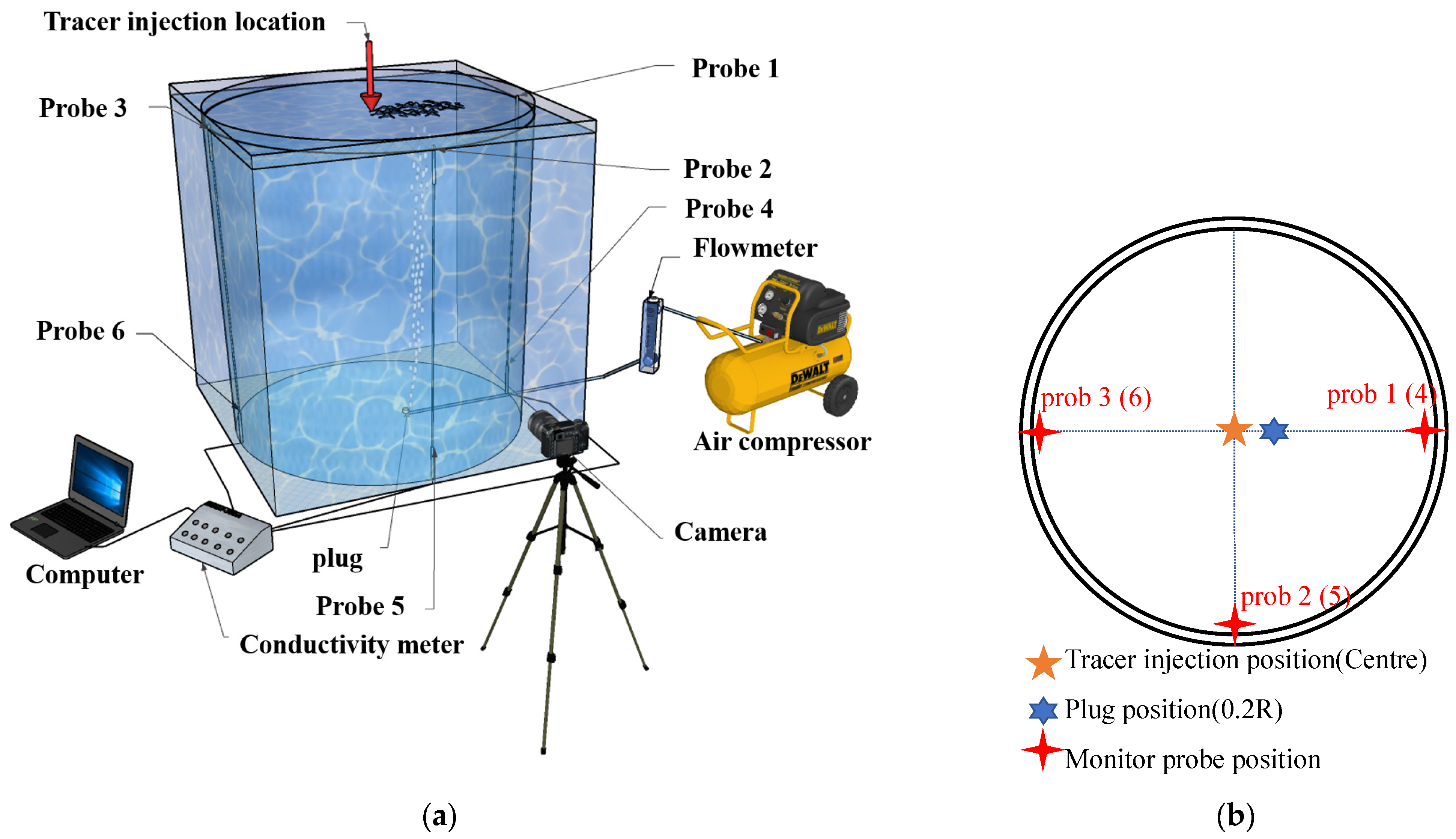
2.2. Experimental Facility

The experimental setup is illustrated in Figure 1. During the experiment, the liquid level of the ladle is kept at 1000 mm, and the porous plug is positioned at a distance of 0.2 R from the center of the ladle’s bottom. Stirring is carried out using single-hole blowing, and the tracer is introduced from the center of the liquid surface. Six monitoring points are designated for the experiment, namely, top monitoring points 1, 2, and 3, located 25 cm below the liquid’s surface, and bottom monitoring points 4, 5, and 6, situated near the bottom wall of the ladle. The mixing time of each monitoring point was determined by using the “stimulus-response” method in the experiment. Upon the addition of the salt solution tracer, electric conductivity data from the six monitoring positions within the ladle were simultaneously collected by using the DDSJ-308A conductivity meter (equipment accuracy: ±0.5% FS). Conductivity data at each monitoring point were obtained for each experimental scheme, further post-processed to the dimensionless concentration curves, and used to calculate mixing times (with a 5% standard for determining the mixing time of each group). Repeated experiments of more than ten trials were performed for each scheme. The mixing times of each trial were obtained, and the averaged mixing time value of the repeated experiments were used for the specific monitoring points. A detailed evaluation of the errors of the averaging mixing time will be discussed in Section 3.1.

2.3. Experimental Scheme

To investigate the influence of tracer dosage on the flow field and mixing time of the ladle, six dosages were designed in the experiment, covering a range of tracer volume-to-water volume ratios from 0.13 × 10⁻³ to 0.97 × 10⁻³, which essentially covers all ranges of tracer-to-water proportions in Table 1. Under these conditions, the variations in electric conductivity (concentration) at each monitoring point were recorded. The studied scheme and dosage of the tracer is presented in

Table 3. Table of dosage range for tracers.

Dosage of Saturated NaCl Solution (mL)	92	185	277	370	463	695
Volume ratio of saturated NaCl solution to water	0.13 × 10−3	0.26 × 10−3	0.39 × 10−3	0.52 × 10−3	0.65 × 10−3	0.97 × 10−3

.

3. Results

3.1. Experimental Error Analysis

Before the experiments, the uncertainty analysis for experimental data is carried out. The error analysis of the experiment primarily includes two aspects: (1) error analysis of dimensionless concentration curves and (2) error analysis of mixing time.

Firstly, to verify the repeatability of the dimensionless concentration curves in multiple trials, the scheme with an injection dosage of 92 mL saturated NaCl solution is taken as an example. In addition, the conductivity values as a function of time at six monitoring points inside the ladle were recorded. The data collected from the repeated trials were post-processed individually, and dimensionless concentration curves were obtained. The maximum and minimum dimensionless concentration data from the repeated trials at each time step interval were recorded as a function of time and plotted as the shaded regions in Figure 2. This method of plotting can be found in a previous paper [65]. In addition, the averaged concentration of repeated trials at each time step interval was processed, and those sets of value are plotted as a function of time as shown in the solid lines in Figure 2. Among them, Figure 2 a–c,e,f correspond to dimensionless concentration curves at monitoring points 1, 2, 3, 5, and 6, respectively. The figures indicate that the fluctuation ranges of the data from the repeated trials at these monitoring points are relatively small compared to the average curves. In Figure 2e, regarding monitoring point 4, the fluctuation range of the dimensionless concentration curves in the repeated trials is relatively large, and two significantly different trends are observed among the trials. The two different curves are of the sinusoidal and parabolic types [43], which represent two types of tracer transport. This will be further explored in Section 3.3.

The average mixing time value obtained from every repeated trial was utilized in this study as the mixing time for a certain monitoring point. To validate the repeatability of the method for calculating mixing time, an error analysis of the method was conducted. Similarly, the scheme using an injection dosage of 92 mL saturated NaCl solution was taken as an example: the mixing time calculated from ten repeated trials was statistically analyzed, and the average values and standard deviations of ten sets of data were calculated.

Table 4. Statistics of mixing time from multiple trials and the averaged mixing time.

Order	1	2	3	4	5	6	7	8	9	10	AVG	S.D.
Time(s)
Monitor
1	44	50	65	45	76	73	62	47	58	76	59.60	12.75
2	65	72	44	56	44	73	68	54	54	50	58.00	10.86
3	103	87	85	102	93	82	91	72	87	87	88.90	9.13
4	84	108	116	89	92	89	102	92	92	93	95.70	9.88
5	103	80	113	86	85	109	107	92	75	116	96.60	14.75
6	87	87	105	98	68	110	72	86	82	66	86.10	14.98

AVG: The average mixing time of ten trials. S.D.: The standard deviation of the mixing time of ten trials.

presents a summary of the mixing times, with statistics conducted for the top monitoring points 1, 2, and 3 as well as the bottom monitoring points 4, 5, and 6. It can be inferred from the table that after averaging the ten sets of data, the average mixing times for the top monitoring points were 59.6 s, 58.0 s, and 88.9 s, with standard deviations of 12.75 s, 10.86 s, and 9.13 s, respectively. The average mixing times for the bottom monitoring points were 95.7 s, 96.6 s, and 86.1 s, with standard deviations of 9.88 s, 14.75 s, and 14.98 s, respectively. By comparing the average mixing times of the six monitoring points with the mixing times obtained from each repeated trial, it was found that the standard deviations all ranged within 15%, indicating acceptable differences between individual mixing times and average mixing times. Therefore, the average mixing time value obtained from ten repeated trials will be utilized as the mixing time in this study.

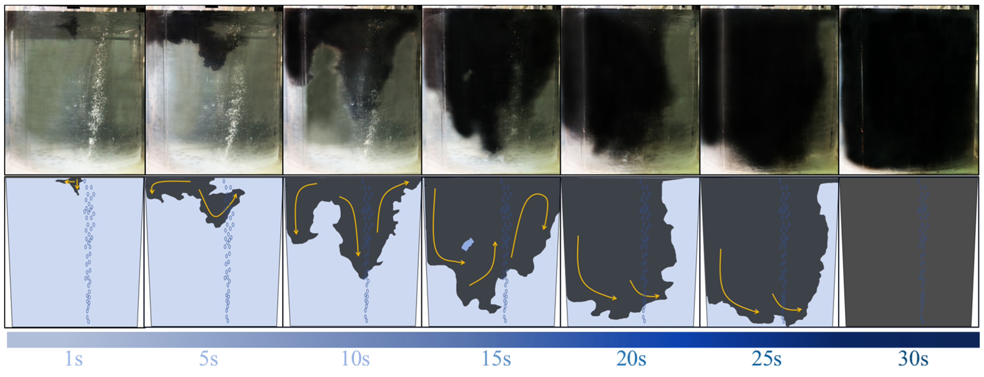
3.2. Transport Path of Tracer

Figure 3 depicts the typical transport process of 100 mL of ink tracer. The tracer is injected from the central position of the ladle’s liquid surface and rapidly diffuses across the surface. Subsequently, the majority of the tracer diffuses from the left side of the ladle to the bottom, then circulates rapidly on the left side. Concurrently, a small portion of the tracer diffuses to the right side of the ladle and spreads downward at a slower rate along the right wall. The tracer on the left side reaches the bottom of the ladle first, then gradually spreads from left to right at the bottom until achieving uniform distribution.

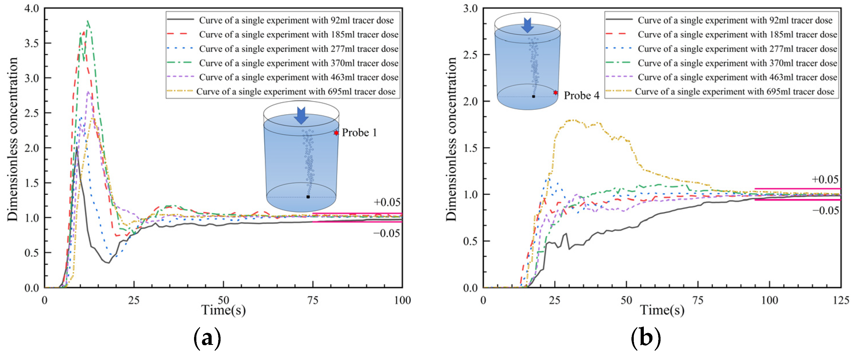
3.3. Analysis of Dimensionless Concentration Curves at Monitoring Points 1 and 4

The dimensionless concentration curves at monitoring point 1 in the ladle water model after the addition of different volumes of saturated NaCl solution is presented in Figure 4a. All of the curves show a sinusoidal tendency. The initial response time of monitoring point 1 falls within the range of 5 s to 6 s with the addition of different volumes of saturated NaCl solution, indicating that the volume of the tracer has no influence on the response time of conductivity at monitoring point 1. In addition, as the volume of the tracer increases, the peak dimensionless concentrations are 2.1, 3.7, 2.5, 3.8, 2.8, and 2.4, with corresponding peak arrival times of 10 s, 12 s, 10 s, 13 s, 13 s, and 14 s, respectively. Therefore, it is concluded that with the increasing tracer volume, the time at which the dimensionless concentration peak occurs at monitoring point 1 is also delayed. Furthermore, the peak values exhibit a first increase followed by a decrease as the volume of the tracer increases. The occurrence of this phenomenon is attributed to the increase in tracer volume, leading to a corresponding rise in salt concentration at monitoring point 1. However, when the volume exceeds a certain threshold, the deposition rate of soluble salt solution is accelerated, leading to its rapid settling at the bottom of the ladle, without sufficient diffusion time to monitoring point 1, thereby causing a delay in the peak time and decrease in peak values. The time interval between the two peak values can be utilized to estimate the approximate duration of one cycle of the tracer’s movement within the ladle water model, which is approximately 20 s. However, given that the dimensionless concentration peak values range between 2 and 4, with minor differences, it can be inferred that monitoring point 1 exhibits insensitivity to changes in tracer volume.

For monitoring point 4, located at the bottom right corner of the ladle, as shown in Figure 4b, the curves show both sinusoidal and parabolic types, as described in Section 3.1. The schemes with a larger tracer volume tend to show a sinusoidal curve while the smaller tracer volume schemes show parabolic curves. For the variation in the dimensionless concentration curves with respect to the volume of salt solution tracer, the tracer is dispersed to monitoring point 4 between 13 and 16 s. The peak value of the dimensionless concentration curve is relatively low, with a maximum value less than 1.8. However, there is a significant difference in the concentration peak values corresponding to different tracer volumes.

Below is an in-depth analysis of the sinusoidal- and parabolic-type curves and their corresponding tracer transport processes. As described in Section 3.2, for the dimensionless concentration curves at monitoring point 4, there are two distinct trends that could be identified under the same experimental conditions: (1) Trend 1 (sinusoidal type) is characterized by a rapid increase in concentration shortly after the onset of the response, followed by a sharp decrease after the emergence of a prominent peak, with a subsequent rise in concentration leading to a second smaller peak. (2) Trend 2 (parabolic type) is characterized by a slower variation in the dimensionless concentration, with no distinct peaks observed in the dimensionless concentration curve.

To investigate the reasons behind the two different trends observed in the dimensionless concentration curves at monitoring point 4, a visualization experiment was designed via injection of a tracer mixture. Specifically, in the water model, the injected tracer is 102 mL of mixed tracer solution (composed of 92 mL of saturated NaCl solution and 10 mL of black ink). The total soluble NaCl concentration is identical to that of the 92 mL saturated NaCl solution. The typical photo and schematic diagrams of ink tracer transport of both trend 1 and trend 2 are shown in Figure 5 and Figure 6, respectively.

In Figure 5, upon the injection of the tracer into the ladle, asymmetrical transport of tracer is observed in two directions: firstly, movement towards the left direction along the main circulation area, and secondly, a vertical downward motion followed by a shift towards the gas column side. At 10 s, the tracer is moved downward along the left sidewall with the main circulation flow, and the tracer’s downward flow towards the gas column side is pushed upward towards the liquid surface due to the gas stirring. Between 15 and 20 s, the tracer following the main circulation intersects with the downward-flow tracer, subsequently gradually settling at the bottom until the ink tracer is mixed in the left side of the ladle. However, the tracer on the right side of the gas column is in a relatively low concentration.

Figure 6 shows trend 2, which differs significantly from Figure 5. Upon injection of tracer, the tracer is transported asymmetrically; i.e., it moves downward along the left side of the ladle following the main circulation flow, predominantly circulating on the left side of the ladle until about 20 s. At 20 s, a portion of the tracer begins to flow upward towards the liquid surface with the gas column. Subsequently, a small portion of the tracer flows downward along the right sidewall following the weak circulation flow on the right side and ultimately reaching the bottom, resulting in thorough mixing in the whole ladle.

The dimensionless concentration curves of trend 1 and trend 2 are shown in Figure 7 and Figure 8, respectively. In trend 1 (corresponding to the sinusoidal-type curve at monitoring point 4), the tracer being injected is subsequently transported in two directions, resulting in a lower peak value (about 20) at monitoring point 3 compared to that in trend 2 (peak value of about 60). At 12 s, due to the effect of gas plumes, the tracer is transported to the right side of the liquid surface, initiating changes in the dimensionless concentration curve at monitoring point 1. Since this point is located closest to the top of the gas plume on the liquid surface, the dimensionless concentration curve exhibits significant fluctuations. This is due to the rapid downward transport of tracers along the right sidewall. At 30 s, the dimensionless concentration at monitoring point 4 begins to rapidly rise, reaching its peak 4 s later. This is due to the large portion of tracer transported to the bottom right side.

In trend 2 (corresponding to parabolic-type curve at monitoring point 4), in contrast to trend 1, a majority of the tracer is transported along the left sidewall without flowing downward or to the right. Consequently, the peak concentration at monitoring point 3 increases rapidly to 60 (significantly higher than that in trend 1). Due to the intensive circulation of the tracer on the left side of the ladle during the initial 20 s, the arrival time of the tracer at monitoring point 1 is delayed compared to that in trend 1. At 33 s, the tracer is transported along the right sidewall to monitoring point 4. Due to the small portion of the tracer being transported to the right side, the dimensionless concentration curve at this monitoring point increases slowly without distinct peaks.

However, the scheme with a tracer volume of 695 mL, as seen in Figure 4b, is an exception since the curve at monitoring point 4 tends to be of the sinusoidal type. In this case, the dimensionless concentration starts to rise at 15 s, with a relatively rapid rise, and reaches a peak concentration of 1.8 at 33 s. After 33 s, the concentration begins to decrease slowly with fluctuations attributed to the salt reaching this position not being quickly transported away but diffusing slowly to other locations until mixing is complete.

The reason why this scheme shows only trend 1 is that the tracer volume is too large, causing it to rapidly move downward after injection into the ladle. A significant portion of the salt solution is deposited at the bottom, gradually diffusing from the bottom center to various positions in the ladle, resulting in a sinusoidal type of concentration curve at monitoring point 4. Furthermore, regardless of the studied schemes, the peak value of the dimensionless concentration curve at monitoring point 4 in Figure 4b does not exceed 2 (compared to the value of 20–60 at point 3), indicating that weak mixing occurs at this point. This also demonstrates that the salt concentration directly transported to this point is not substantial, and it is mainly transported to point 4 by circulating flow streams or slow diffusion from the bottom.

In all studied tracer volume schemes, the response time of monitoring point 4 is around 1 s to 15 s. The occurrence of the two trends is exclusive to monitoring point 4 because it is located on the bottom side of the plug. It is pointed out that this area is an inactive or dead zone [73]. In summary, the main pathway for the tracer to be transported to this area is not singular, resulting in a much more complex mixing process and mixing time compared to other positions.

3.4. Analysis of Dimensionless Concentration Curves at Monitoring Points 2 and 5

Figure 9a shows the dimensionless concentration curves at monitoring point 2 after the injection of saturated NaCl solutions of different volumes. Similar to the results at monitoring point 1, all of the curves at monitoring point 2 show a sinusoidal tendency. The response time at monitoring point 2 is around 5 s. Furthermore, except for the scheme with the largest volume of 695 mL solution, the dimensionless concentration reaches its maximum value at approximately 13 s. The concentration peak for this scheme is delayed for only 2 s. This situation may be attributed to the rapid settling of the salt solution due to the excessively large tracer volume, ultimately resulting in a delay in the arrival time of the salt solution at monitoring point 2. With increased tracer volume, the peak values of the dimensionless concentration curves are 3.7, 3.2, 5.1, 4.5, 3.9, and 2.6, respectively. The peak values of the concentration curves showed a trend of increasing first and then decreasing. This trend is also attributed to the settling of the salt solution caused by the increased tracer volume. Overall, the influence of tracer volume variations on the dimensionless concentration curves at this point is insignificant, and this tendency is similar to that observed at monitoring point 1. By observing the dimensionless concentration curves of six sets of schemes, it was found that the second peak occurs between 26 and 34 s, and the time interval between the two peaks varies between 16 and 20 s. Hence, it can be inferred that the circulation passing through monitoring point 2 in the ladle takes approximately 16 to 20 s to complete one cycle, indicating a slightly shorter circulation time than that observed at monitoring point 1 (20 s).

Figure 9b shows the dimensionless concentration curves at monitoring point 5. When the tracer volume is 695 mL, the curve shows a sinusoidal tendency, while in the other schemes, the curves are of the parabolic type. For the scheme with a tracer volume of 695 mL, a rapidly rising trend is exhibited. The response time is 15 s, and the peak time is 26 s. The peak value is 1.96. Subsequently, fluctuations are observed in the dimensionless concentration curve instead of a rapid decrease, with a second peak with a value of 1.58 observed at 40 s and a third peak with a value of 1.17 at 66 s. The dimensionless concentration gradually decreases to unity thereafter. For the six different schemes, the response times for the dimensionless concentration curves are 18 s, 18 s, 21 s, 18 s, 14 s, and 15 s, respectively. The response time at monitoring point 5 is shortened by the increase in tracer volume. This phenomenon can be attributed to the accelerated downward transport of the tracer caused by the increased volume, resulting in faster settling and an earlier response time at the bottom monitoring point 5. However, when the tracer volume is 695 mL, a significant deviation from the other schemes’ curves is observed. This difference mainly arises from the excessive tracer volume, which hinders the transport of the tracer within the ladle, resulting in substantial deposition of tracer at the bottom before gradually diffusing to that location. Consequently, the dimensionless concentration curve is not observed to decrease rapidly after reaching its peak; instead, it gradually decreases while still displaying several smaller peaks.

3.5. Analysis of Dimensionless Concentration Curves at Monitoring Points 3 and 6

Figure 10a shows the dimensionless concentration curve at monitoring point 3. All of the curves show a sinusoidal tendency, which is similar to the results at point 1 and point 2. It is obvious that the curve of the scheme with the largest tracer volume shows a strong tendency to shift to the right side compared to the curves of the other schemes. Apart from this scheme, the curves of the other schemes are similar. It is noted that the response time of conductivity at monitoring point 3 remains around 5 s. Moreover, the curve of the scheme with the smallest tracer volume shows a very sharp peak compared to the other schemes. It is observed that the first peak value of the concentration curve generally decreases with the increase in tracer volume. For the small tracer volume scheme, the tracer follows the main circulation, and a large portion of the tracer is rapidly transported to monitoring point 3. However, as the tracer volume increases, the tracer first moves downward for a certain distance (as shown in Figure 5). During this period, the flow field in the water model of the ladle is temporarily disturbed, leading to the salt solution’s deposition at the bottom of the ladle. For this scheme, only a limited portion of the tracer is transported to point 3, and a smaller peak value in the concentration curve is observed. The time interval between the two peak values for different schemes ranges from 12 to 15 s, which is slightly shorter than that at monitoring point 2 and point 1. The time interval between the two peaks decreases as the tracer volume increases.

In Figure 10a, as noted, the curve in the scheme with a tracer volume of 695 mL showed a shifting tendency with a response time of 15 s. The curve does not display a distinct peak and exhibits slow changes in dimensionless concentration before 20 s, followed by a rapid increase after that time, reaching its maximum value at 28 s. Furthermore, unlike the other five curves at this monitoring point, this curve does not exhibit a rapid decrease after reaching its peak value; instead, it slowly decreases with some fluctuations. This situation can also be attributed to the accelerated downward transport of the tracer caused by the increased volume of the salt solution tracer.

Figure 10b shows the dimensionless concentration curve at monitoring point 6. All of the curves show a smooth sinusoidal tendency, and some are close to the parabolic type. Unlike the results at monitoring points 4 and 5, the consistency of the curves between different schemes is very good. A slight difference is that the scheme with the smallest tracer injection volume showed a slower increase in concentration and a fluctuating curve.

3.6. Mixing Time

The scatter plots in Figure 11a,b depict the average mixing time at every monitoring point of various tracer volume schemes. The mixing times in the figure are determined by using the 95% criterion. It is noted that shorter mixing times are observed at most of the top monitoring points compared to the bottom monitoring points. Additionally, a decreasing tendency with increasing tracer volume is observed for the top monitoring points, followed by a slight increase in the mixing time at higher tracer volumes. The transition from decreasing to increasing occurs at the x-axis of the 370 mL tracer volume. In addition, the mixing times at the bottom monitoring points decrease with the increase in the tracer volume.

The maximum mixing time, which represents the longest recorded mixing time across the six monitoring points, is displayed in Figure 12. The maximum or ultimate mixing times corresponding to tracer volumes ranging from 92 mL to 695 mL are 97.1 s, 96.7 s, 84.6 s, 80.6 s, 80.95 s, and 80.5 s, respectively. It is clear that the ultimate mixing time decreases with the increase in tracer volume.

The variations in average mixing times at various monitoring points with the volume of the injected salt solution tracer were summarized and re-plotted into a three-dimensional graph, as shown in Figure 13. From the graph, it is visually evident that the range of mixing times spans from 54 s to 97 s. Among all experimental schemes, the mixing time at monitoring point 3 exhibits the longest value when the volume of the tracer is 92 mL. In the same scheme, the mixing time is also relatively long, approximately 90 s, at monitoring points 4, 5, and 6. When the tracer volume is 370 mL, the mixing time at the upper monitoring points showed the shortest value compared to the other schemes. The mixing time at the three bottom monitoring points are similar, and are approximately 78 s.

It is evident that the mixing times at the top monitoring points are shorter than those at the bottom monitoring points. When comparing the results of different monitoring points, the mixing time at monitoring point 1 is the shortest. Additionally, in the three-dimensional graph, it can be observed that the surrounding areas are higher than the central area, indicating a trend of decreasing and then increasing mixing times for each monitoring point as the tracer volume increases. This tendency is more obvious for top monitoring points, as described in previous sections. The transition of mixing time at the top monitoring points from decrease to increase occurs when the volume of the tracer reaches 370 mL. Furthermore, regardless of the tracer volume used, the mixing times at the bottom monitoring points are consistently higher than those at the top monitoring points.

4. Discussions

(1) Based on the analysis of tracer transport paths in Section 3.2, it was observed that after the injection of 100 mL of black ink tracer at the exact center of the liquid’s surface, under the influence of bottom-blowing gas, the majority of the tracer is asymmetrically transported towards the left sidewall of the ladle, with diffusion towards the center of the ladle occurring during the circulation process. Note that this is a black ink tracer whose density is very close to that of water. For the denser NaCl solution tracer, as presented in Section 3.3, there are two distinct trends that could be identified under the same experimental conditions. Trend 2 is similar to the asymmetric tracer transport observed in the black ink tracer schemes. However, in trend 1, in which the gas plume oscillates, the injected tracer is transported both by the main circulation to the left sidewall and by a downward flow towards the gas column. This downward flow is beneficial for quick mixing in the whole ladle. Thereafter, the tracer disperses to the monitor 4 on the bottom right side at a rapid pace. This is the reason why sinusoidal-type concentration curves are observed at monitoring point 4 in trend 1. In contrast, the slow diffusion of the tracer from the left side results in the parabolic-type concentration curves of trend 2. The above results indicate that differences in tracer density/concentration significantly influence the tracer’s transport path within the ladle. Furthermore, as the tracer volume increases, it further impacts the original flow field within the ladle by accelerating the downward flow.

(2) The mixing performance at different monitoring points was widely studied in 1980s by Oeters and co-workers [76,77,78,79,80,81]. In 1988, Krishna-Murthy et al. [82] concluded that the mixing time did not depend on the variations in the amount of tracer used. However, the effect of a salt solution tracer on the mixing in a ladle was possibly first observed by Chen et al. [71] in 2013. The conclusion of this study is that the mixing time decreased with the increase in the saturated salt solution tracer volume. However, unfortunately, the results of [71] are merely based on the monitoring points at the top surface of the ladle. Moreover, the transport of salt solution tracers was not visualized in this study. In the present study, the mixture of ink and salt solution tracers was used to visualize the transport of tracers, and two distinct trends were discovered possibly for the first time. In addition, in this study, the mixing time at the upper monitoring points exhibited a trend of initially decreasing followed by increasing with the increase in tracer volume. The reasons underlying the disparities between the results of this study and those of Chen et al. [71] warrant further investigation.

(3) The stirring gas flow rates vary in different ladle operations. In 2018, Gómez et al. [72] explored the impact of salt solution tracer concentration (equivalent to the volume change) and gas flow rate on the measured mixing time, affirming that tracer concentration indeed exerts a direct influence on mixing time, particularly at lower gas flow rates. They found that, at higher gas flow rates, this influence may be negligible. However, when converted to normal operating conditions, the lower gas flow rate mentioned in Gómez et al. [72] is 610 NL·min⁻¹. This flow rate is relatively large compared to most experiments and production processes. Consequently, the so-called low gas flow rate used by Gómez et al. [72] is not that low and, in fact, represents a moderate or moderately high gas flow rate. Further research is needed to better understand the effects of density/concentration variations on flow fields and mixing times at low gas flow rates.

(4) Regarding the results for water model studies, Chen et al. [71] proposed an optimized dimensionless tracer amount (dosage) of 0.2692 × 10⁻³ when a 5% mixing criterion was used. In the study of Chen et al. [71], they referred to the results from [83] and addressed the fluctuation in concentration when an extremely small dosage of salt solution tracer was injected. The fluctuation in concentration (following small input tracer dosage) makes identifying the mixing time value tough. Distinguishing the difference between fluctuations in concentrations and the concentration evaluation range by either 5% or 1% is challenging. In the present study, the mixing times of the schemes with 92 mL and 185 mL tracer volumes were relatively longer than those of the other schemes. The corresponding dimensionless tracer volumes (dosage) are 0.13 × 10⁻³ and 0.26 × 10⁻³, respectively. So far, we cannot conclude that the use of a sufficiently low dosage (concentration) of salt solution tracer is the optimal operation. It can be understood from this study that when the dimensionless tracer dosage is as large as 0.39 × 10⁻³, the measured mixing time values vary in a limited range. However, knowing what we are measuring and the fluid mechanics behind the data were our motivations in this paper. When setting up water modeling of ladles and using these data for validation of computational fluid dynamics simulations, researchers should be aware of this phenomenon.

5. Concluding Remarks

The following conclusions can be summarized:

• An uncertainty analysis for the experimental data was carried out. The ratio of the standard deviations of the repeated trials to the averaged mixing times ranged within 15%.
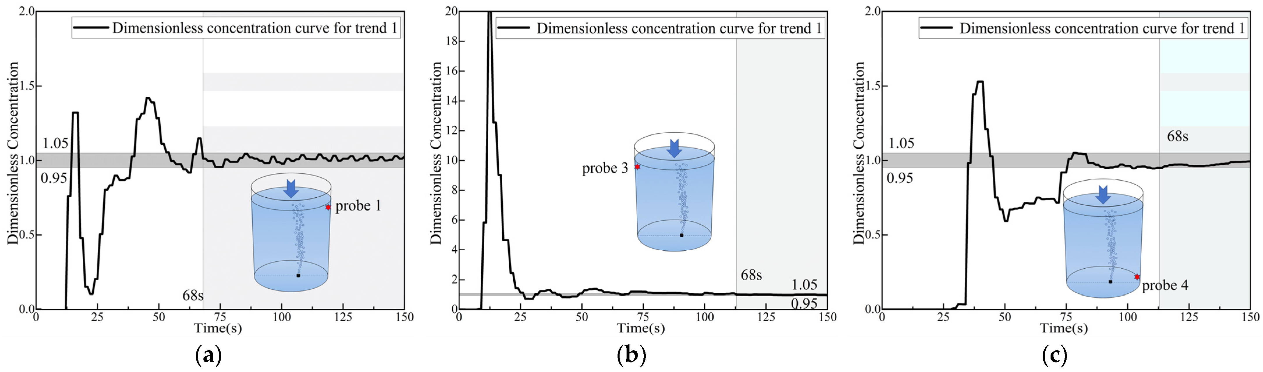
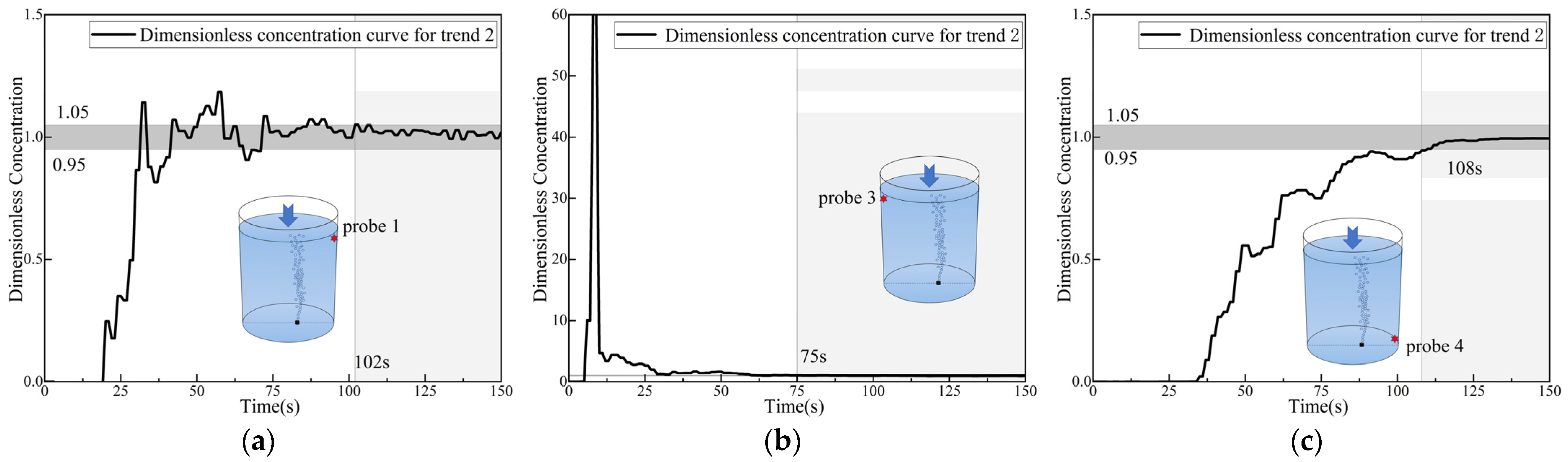
• For the dimensionless concentration curves, sinusoidal-type curves, which represent rapid mixing, are observed at the top monitoring points. Meanwhile, parabolic-type curves, which represent slow mixing by diffusion, are observed at the bottom monitoring points. An exception is the monitoring point at the bottom right side (close to the asymmetric gas nozzle area), where two distinct trends, both sinusoidal and parabolic, were observed at this point.
• After a well-designed visualization experiment involving the mixture of salt solution and ink tracers, two trends of asymmetrical transport of the tracer were observed. In the first trend, the injection of the tracer occurred during the oscillation of the gas plume. The injected salt solution tracer was transported both by the main circulation to the left sidewall and by downward flow towards the gas column. The downward flow was accelerated and became a major flow pattern when the tracer volume increased. For the second trend, which can also be observed in the lighter-density ink tracer scheme, the injected salt solution tracer was asymmetrically transported towards the left sidewall of the ladle by the main circulation.
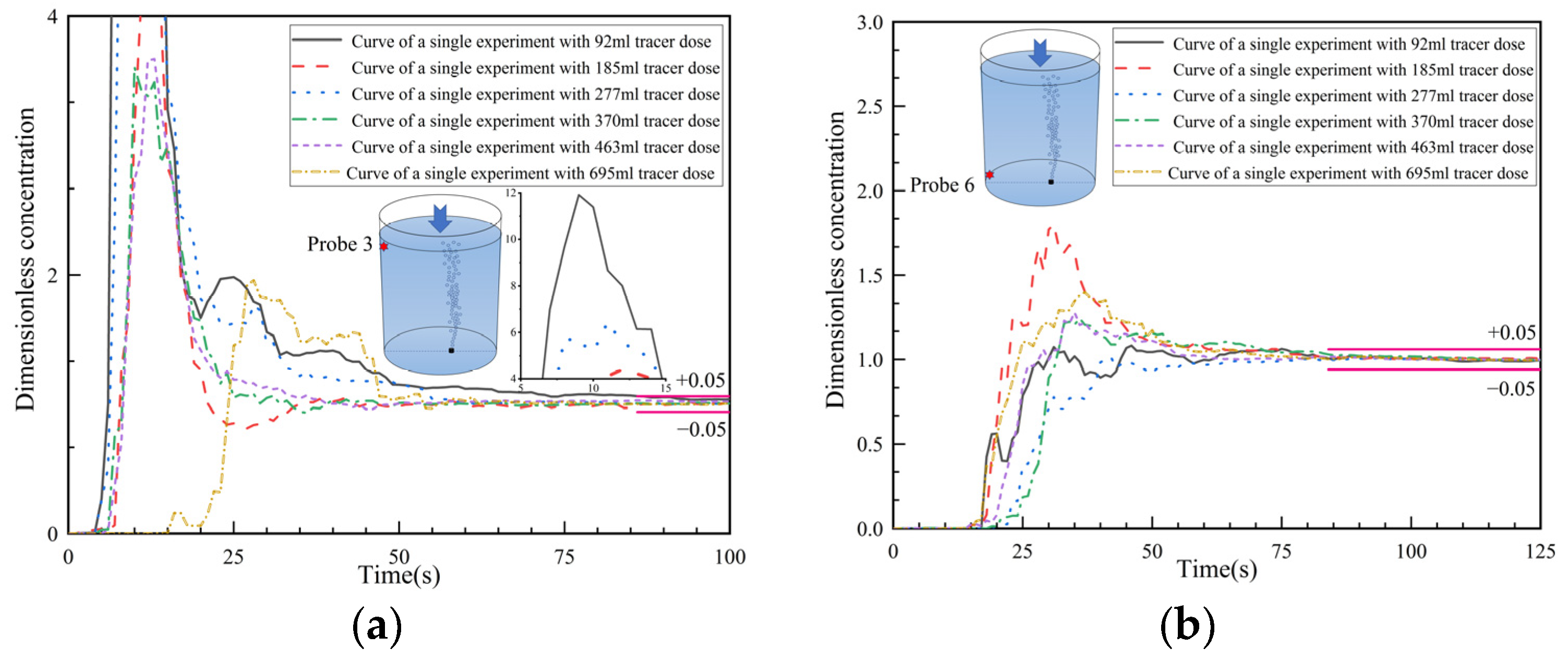
• The response time, peak time, peak concentrations, second/third peaks, and the overall concentration curve types are described in the text. The details of the curves and the ink visualizations can be used to illustrate the transport of salt solution tracers with different dosages/volume. Overall, the curves at the top surface monitoring points are less influenced by the tracer volume, except for the monitoring point at the upper left side. In this area, the portion of the transported salt solution varies in the two trends, i.e., the transported tracer portion is significant in trend 1 but minor in trend 2. The curves at the bottom monitoring points are notably influenced by the tracer volume, since the downward flow intensity varied across different schemes. As a result, the salt concentration is deposited at the bottom with a slow subsequent diffusion.
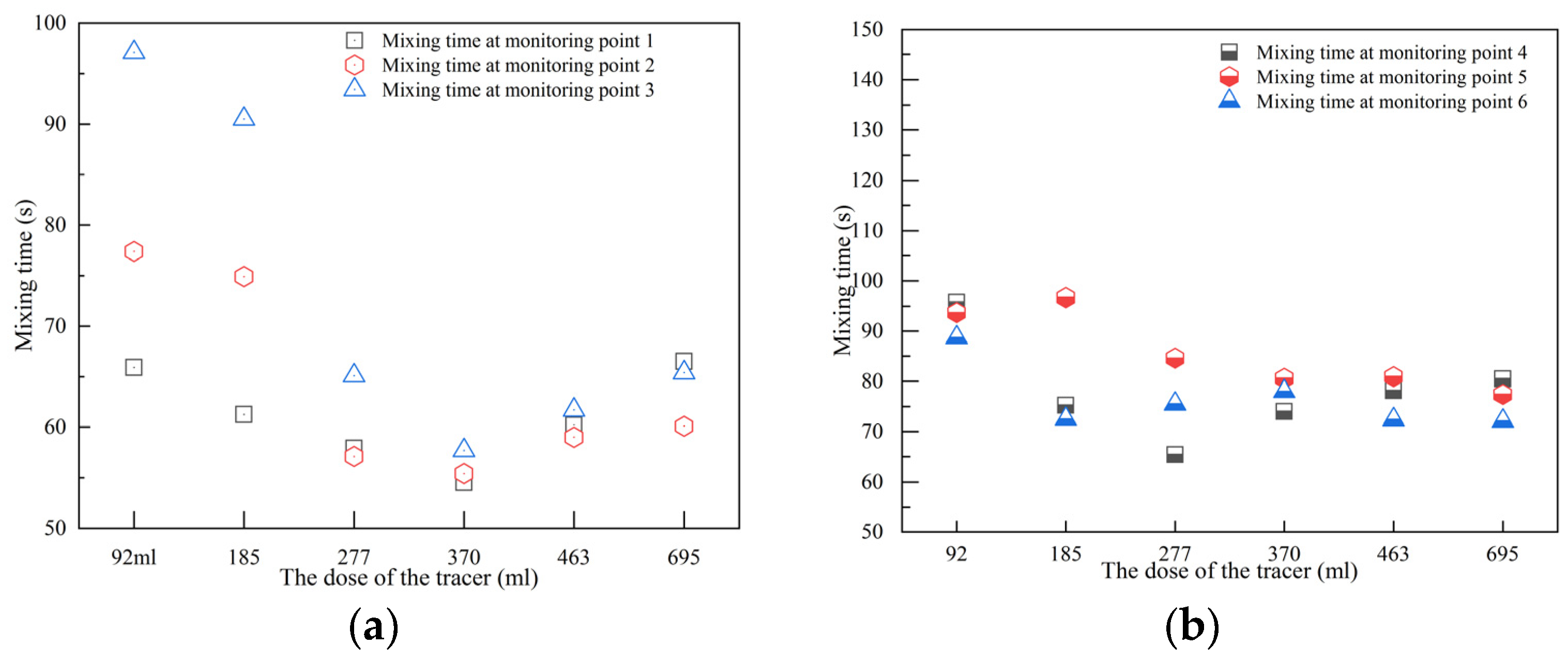
• For the overall mixing time, a trend of decreasing and then increasing as the tracer volume increases was found at the top monitoring points. The transition tracer volume is 370 mL. Meanwhile, the mixing times at the bottom monitoring points decrease with the increase in tracer volume.
• It is noted that the results are based on moderate gas flow rate conditions. Further studies on the gas flow rate conditions are required, which we have completed and our results will be available soon.

References

1. Szekely, J.; Carlsson, G.; Helle, L. Ladle Metallurgy; Springer: Berlin/Heidelberg, Germany, 1989; pp. 27–71. [Google Scholar]
2. Mazumdar, D.; Guthrie, R.L. The physical and mathematical modelling of gas stirred ladle systems. ISIJ Int. 1995, 35, 1–20. [Google Scholar] [CrossRef]
3. Jönsson, P.; Jonsson, L.I. The Use of Fundamental Process Models in Studying Ladle Refining Operations. ISIJ Int. 2001, 41, 1289–1302. [Google Scholar] [CrossRef]
4. Mazumdar, D.; Evans, J.W. Macroscopic Models for Gas Stirred Ladles. ISIJ Int. 2004, 44, 447–461. [Google Scholar] [CrossRef]
5. Xin, Z.; Zhang, J.; Peng, K.; Zhang, J.; Zhang, C.; Liu, Q. Modeling of LF refining process: A review. J. Iron Steel Res. Int. 2024, 31, 289–317. [Google Scholar] [CrossRef]
6. Niu, K.; Feng, W.; Conejo, A.N.; Ramírez-Argáez, M.A.; Yan, H. 3D CFD Model of Ladle Heat Transfer with Gas Injection. Metall. Mater. Trans. B 2023, 54, 2066–2079. [Google Scholar] [CrossRef]
7. Conejo, A.N. Physical and Mathematical Modelling of Mass Transfer in Ladles due to Bottom Gas Stirring: A Review. Processes 2020, 8, 750. [Google Scholar] [CrossRef]
8. Niu, K.; Feng, W.; Conejo, A.N. Effect of the Nozzle Radial Position and Gas Flow Rate on Mass Transfer during Bottom Gas Injection in Ladles with One Nozzle. Metall. Mater. Trans. B 2022, 53, 1344–1350. [Google Scholar] [CrossRef]
9. Ji, S.; Niu, K.; Conejo, A.N. Multiphase modeling of steel-slag mass transfer through distorted interface in bottom-stirred ladle. ISIJ Int. 2024, 64, 52–58. [Google Scholar] [CrossRef]
10. Podder, A.; Coley, K.S.; Phillion, A.B. Modeling Study of Steel–Slag–Inclusion Reactions During the Refining of Si–Mn Killed Steel. Steel Res. Int. 2022, 94, 2100831. [Google Scholar] [CrossRef]
11. Podder, A.; Coley, K.S.; Phillion, A.B. Simulation of Ladle Refining Reactions in Si–Mn-Killed Steel. Steel Res. Int. 2024. Available online: https://onlinelibrary.wiley.com/doi/full/10.1002/srin.202300330 (accessed on 26 March 2024). [CrossRef]
12. Duan, H.; Zhang, L.; Thomas, B.; Conejo, A.N. Fluid Flow, Dissolution, and Mixing Phenomena in Argon-Stirred Steel Ladles. Metall. Mater. Trans. B 2018, 49, 2722–2743. [Google Scholar] [CrossRef]
13. Duan, H.; Zhang, L.; Thomas, B.G. Effect of melt superheat and alloy size on the mixing phenomena in argon-stirred steel ladles. Steel Res. Int. 2019, 90, 1800288. [Google Scholar] [CrossRef]
14. Liu, C.; Peng, K.Y.; Wang, Q.; Li, G.Q.; Wang, J.J.; Zhang, L.F. CFD Investigation of Melting Behaviors of Two Alloy Particles During Multiphase Vacuum Refining Process. Metall. Mater. Trans. B 2023, 54, 2174–2187. [Google Scholar] [CrossRef]
15. Yang, R.; Chen, C.; Lin, Y.; Zhao, Y.; Zhao, J.; Zhu, J.; Yang, S. Water model experiment on motion and melting of scarp in gas stirred reactors. Chin. J. Process Eng. 2022, 22, 954–962. [Google Scholar] [CrossRef]
16. Li, X.; Wang, H.; Tian, J.; Wang, D.; Qu, T.; Hou, D.; Hu, S.; Wu, G. Investigation on the Alloy Mixing and Inclusion Removement through Using a New Slot-Porous Matched Tuyeres. Metals 2023, 13, 667. [Google Scholar] [CrossRef]
17. Wen, X.; Ren, Y.; Zhang, L. Effect of CaF2 Contents in Slag on Inclusion Absorption in a Bearing Steel. Steel Res. Int. 2022, 94, 2200218. [Google Scholar] [CrossRef]
18. Kim, T.S.; Yang, J.; Park, J.H. Effect of Physicochemical Properties of Slag on the Removal Rate of Alumina Inclusions in the Ruhrstahl–Heraeus (RH) Refining Conditions. Metall. Mater. Trans. B 2022, 53, 2523–2533. [Google Scholar]
19. Li, X.; Hu, S.; Wang, D.; Qu, T.; Wu, G.; Zhang, P.; Quan, Q.; Zhou, X.; Zhang, Z. Inclusion Removements in a Bottom-Stirring Ladle with Novel Slot-Porous Matched Dual Plugs. Metals 2022, 12, 162. [Google Scholar] [CrossRef]
20. Sun, Y.; Duan, H.; Zhang, L. A boundary layer model for capture of inclusions by steel–slag interface in a turbulent flow. J. Iron Steel Res. Int. 2023, 30, 1101–1108. [Google Scholar] [CrossRef]
21. Huang, C.; Duan, H.; Zhang, L. Modeling of Motion of Inclusions in Argon-Stirred Steel Ladles. Steel Res. Int. 2024, 96, 2300537. Available online: https://onlinelibrary.wiley.com/doi/full/10.1002/srin.202300537 (accessed on 26 March 2024). [CrossRef]
22. Qiao, T.; Cheng, G.; Huang, Y.; Li, Y.; Zhang, Y.; Li, Z. Formation and Removal Mechanism of Nonmetallic Inclusions in 42CrMo4 Steel during the Steelmaking Process. Metals 2022, 12, 1505. [Google Scholar] [CrossRef]
23. Zhong, H.; Jiang, M.; Wang, Z.; Zhen, X.; Zhao, H.; Li, T.; Wang, X. Formation and Evolution of Inclusions in AH36 Steel During LF–RH–CC Process: The Influences of Ca-Treatment, Reoxidation, and Solidification. Metall. Mater. Trans. B 2023, 54, 593–601. [Google Scholar] [CrossRef]
24. Ocampo Vaca, F.A.; Hernández Bocanegra, C.A.; Ramos Banderas, J.Á.; Herrera-Ortega, M.; López Granados, N.M.; Solorio Díaz, G. Effect of Ladle Shroud Blockage on Flow Dynamics and Cleanliness of Steel in Coupled Ladle–Shroud–Tundish System. Steel Res. Int. 2024. Available online: https://onlinelibrary.wiley.com/doi/full/10.1002/srin.202300616 (accessed on 13 March 2024). [CrossRef]
25. Conejo, A.N.; Kitamura, S.; Maruoka, N.; Kim, S.J. Effects of Top Layer, Nozzle Arrangement, and Gas Flow Rate on Mixing Time in Agitated Ladles by Bottom Gas Injection. Metall. Mater. Trans. B 2013, 44, 914–923. [Google Scholar] [CrossRef]
26. Terrazas, M.S.C.; Conejo, A.N. Effect of Nozzle Diameter on Mixing Time During Bottom-Gas Injection in Metallurgical Ladles. Metall. Mater. Trans. B 2014, 45, 711–718. [Google Scholar] [CrossRef]
27. Feng, W.; Conejo, A.N. Physical and Numerical Simulation of the Optimum Nozzle Radial Position in Ladles with One Nozzle and Bottom Gas Injection. ISIJ Int. 2022, 62, 1211–1221. [Google Scholar] [CrossRef]
28. Conejo, A.N.; Feng, W. Ladle Eye Formation Due to Bottom Gas Injection: A Reassessment of Experimental Data. Metall. Mater. Trans. B 2022, 53, 999–1017. [Google Scholar] [CrossRef]
29. Wondrak, T.; Timmel, K.; Bruch, C.; Gardin, P.; Hackl, G.; Lachmund, H.; Lüngen, H.B.; Odenthal, H.J.; Eckert, S. Large-Scale Test Facility for Modeling Bubble Behavior and Liquid Metal Two-Phase Flows in a Steel Ladle. Metall. Mater. Trans. B 2022, 53, 1703–1720. [Google Scholar] [CrossRef]
30. Wang, R.; Jin, Y.; Cui, H. The Flow Behavior of Molten Steel in an RH Degasser Under Different Ladle Bottom Stirring Processes. Metall. Mater. Trans. B 2022, 53, 342–351. [Google Scholar] [CrossRef]
31. Jojo-Cunningham, Y.; Guo, X.; Zhou, C.; Liu, Y. Volumetric Flow Field inside a Gas Stirred Cylindrical Water Tank. Fluids 2024, 9, 11. [Google Scholar] [CrossRef]
32. Chen, C.; Cheng, G.G.; Yang, H.K.; Hou, Z.B. Physical Modeling of Fluid Flow Characteristics in a Delta Shaped, Four-Strand Continuous Casting Tundish with Different Flow Control Devices. Adv. Mater. Res. 2011, 284, 1071–1079. [Google Scholar]
33. Schwarz, M.P.; Koh, P.T.L. Numerical Modelling of Bath Mixing by Swirled Gas Injection. In Proceedings of the SCANINJECT IV-4th International Conference on Injection Metallurgy, MEFOS, Luleå, Sweden, 11–13 July 1986. Part I, paper 6. [Google Scholar]
34. Schwarz, M.P.; Turner, W.J. Applicability of the standard k-ϵ turbulence model to gas-stirred baths. Appl. Math. Model. 1988, 12, 273–279. [Google Scholar] [CrossRef]
35. Nick, R.S.; Teng, L.; Yang, H.; Tilliander, A.; Glaser, B.; Sheng, D.Y.; Jönsson, P.G.; Björkvall, J. Mathematical modelling of novel combined stirring method during the final stage of ladle refining. Ironmak. Steelmak. 2023, 50, 721–733. [Google Scholar] [CrossRef]
36. Wang, J.; Ni, P.; Chen, C.; Ersson, M.; Li, Y. Effect of gas blowing nozzle angle on multiphase flow and mass transfer during RH refining process. Int. J. Miner. Metall. Mater. 2023, 30, 844–856. [Google Scholar] [CrossRef]
37. Li, X.; Wang, D.; Tian, J.; Wang, H.; Qu, T.; Hou, D.; Hu, S.; Zhang, Z.; Zhou, X.; Wu, G. Modeling of Bubble Transportation, Expansion, as Well as Adhesion of Inclusions in a Ladle With Different Tuyeres. Metall. Mater. Trans. B 2024, 55, 14–31. [Google Scholar] [CrossRef]
38. Zhou, X.; Zhang, Y.; He, Q.; Ni, P.; Yue, Q.; Ersson, M. Novel Evaluation Method to Determine the Mixing Time in a Ladle Refining Process. Metall. Mater. Trans. B 2022, 53, 4114–4123. [Google Scholar] [CrossRef]
39. Hua, C.; Bao, Y.; Wang, M. Multiphysics numerical simulation model and hydraulic model experiments in the argon-stirred ladle. Processes 2022, 10, 1563. [Google Scholar] [CrossRef]
40. Tiwari, R.; Girard, B.; Labrecque, C.; Isac, M.M.; Guthrie, R.I.L. CFD Predictions for Mixing Times in an Elliptical Ladle Using Single- and Dual-Plug Configurations. Processes 2023, 11, 1665. [Google Scholar] [CrossRef]
41. Schwarz, M.P. Buoyancy and expansion power in gas-agitated baths. ISIJ Int. 1991, 31, 947–951. [Google Scholar] [CrossRef]
42. Schwarz, M.P.; Dang, P. Simulation of Blowthrough in Smelting Baths with Bottom Gas Injection. In Proceedings of the 13th Process Technology Conference Proceedings, ISS, Nashville, TN, USA, 2–5 April 1995; pp. 415–421. [Google Scholar]
43. Ramírez-López, A. Analysis of Mixing Efficiency in a Stirred Reactor Using Computational Fluid Dynamics. Symmetry 2024, 16, 237. [Google Scholar] [CrossRef]
44. Ramírez-López, A.A. Analysis of the Hydrodynamics Behavior Inside a Stirred Reactor for Lead Recycling. Fluids 2023, 8, 268. [Google Scholar] [CrossRef]
45. Jauhiainen, A.; Jonsson, L.; Sheng, D. Modelling of alloy mixing into steel: The influence of porous plug placement in the ladle bottom on the mixing of alloys into steel in a gas-stirred ladle. A comparison made by numerical simulation. Scand. J. Metall. 2001, 30, 242–253. [Google Scholar] [CrossRef]
46. Ganguly, S.; Chakraborty, S. Numerical modelling studies of flow and mixing phenomena in gas stirred steel ladles. Ironmak. Steelmak. 2008, 35, 524–530. [Google Scholar] [CrossRef]
47. Taylor, I.F.; Dang, P.; Schwarz, M.P.; Wright, J.K. An Improved Method for the Experimental Validation of Numerical Mixing Time Predictions. In Proceedings of the 72nd Steelmaking Proceedings, ISS, Chicago, IL, USA, 2–5 April 1989; pp. 505–516. [Google Scholar]
48. Pan, S.; Chiang, J.D.; Hwang, W.S. Effects of gas injection condition on mixing efficiency in the ladle refining process. J. Mater. Eng. Perform 1997, 6, 113–117. [Google Scholar] [CrossRef]
49. Wen, D.; Li, J.; Xie, C.; Tang, H.; Zhang, L.; Wang, Z. Physical model of 150 t ladle refining process. J. Univ. Sci. Technol. Beijing 2007, 29, 101–104. [Google Scholar] [CrossRef]
50. Ek, M.; Wu, L.; Valentin, P.; Sichen, D. Effect of Inert Gas Flow Rate on Homogenization and Inclusion Removal in a Gas Stirred Ladle. ISIJ Int. 2010, 81, 1056–1063. [Google Scholar] [CrossRef]
51. Liu, Y.; Bai, H.; Liu, H.; Ersson, M.; Jönsson, P.G.; Gan, Y. Physical and Numerical Modelling on the Mixing Condition in a 50 t Ladle. Metals 2019, 9, 1136. [Google Scholar] [CrossRef]
52. Tan, F.; He, Z.; Jin, S.; Pan, L.; Li, Y.; Li, B. Physical Modeling Evaluation on Refining Effects of Ladle with Different Purging Plug Designs. Steel Res. Int. 2020, 91, 1900606. [Google Scholar] [CrossRef]
53. Aguilar, G.; Solorio-Diaz, G.; Aguilar-Corona, A.; Ramos-Banderas, J.A.; Hernández, C.A.; Saldaña, F. Study of the Effect of a Plug with Torsion Channels on the Mixing Time in a Continuous Casting Ladle Water Model. Metals 2021, 11, 1942. [Google Scholar] [CrossRef]
54. Conejo, A.N.; Zhao, G.; Zhang, L. On the Limits of the Geometric Scale Ratio Using Water Modeling in Ladles. Metall. Mater. Trans. B 2021, 52, 2263–2274. [Google Scholar] [CrossRef]
55. Shi, P.; Tian, Y.; Xu, L.; Guo, W.; Qiu, S. Physical simulation of 120 t ladle bottom blown argon gas. China Metall. 2021, 31, 30–36. [Google Scholar] [CrossRef]
56. Herrera-Ortega, M.; Ramos-Banderas, J.Á.; Hernández-Bocanegra, C.A.; Montes-Rodríguez, J.J. Effect of the location of tracer addition in a ladle on the mixing time through physical and numerical modeling. ISIJ Int. 2021, 61, 2185–2192. [Google Scholar] [CrossRef]
57. Cheng, R.; Zhang, L.; Yin, Y.; Zhang, J. Effect of side blowing on fluid flow and mixing phenomenon in gas-stirred ladle. Metals 2021, 11, 369. [Google Scholar] [CrossRef]
58. Wang, X.; Zheng, S.; Zhu, M. Optimization of the Structure and Injection Position of Top Submerged Lance in Hot Metal Ladle. ISIJ Int. 2021, 61, 792–801. [Google Scholar] [CrossRef]
59. Wu, W.; Dong, J.; Wei, G. Physical Simulation of Bottom Blowing Argon in 150t Ladle. Contin. Cast. 2022, 2, 45–48. [Google Scholar] [CrossRef]
60. Li, Z.; Ouyang, W.; Wang, Z.; Zheng, R.; Bao, Y.; Gu, C. Physical Simulation Study on Flow Field Characteristics of Molten Steel in 70t Ladle Bottom Argon Blowing Process. Metals 2023, 13, 639. [Google Scholar] [CrossRef]
61. Shan, Q.; Sun, Y.; Duan, H.; Li, Z.; Jia, N.; Chen, W. Water modeling on the transport phenomenon during bottom gas injection of a 210 t ladle. Steelmaking 2023, 39, 35–43. [Google Scholar]
62. Li, L.; Chen, C.; Wang, J.; Tao, X.; Liu, T.; Zhao, Y.; Rong, Z. Flow field optimization and analysis on inclusion removal in elliptical ladle. China Metall. 2024. Available online: https://link.cnki.net/urlid/11.3729.TF.20240407.1139.001 (accessed on 12 April 2024). [CrossRef]
63. Chen, C.; Cheng, G.; Sun, H.; Hou, Z.; Wang, X.; Zhang, J. Effects of Salt Tracer Amount, Concentration and Kind on the Fluid Flow Behavior in a Hydrodynamic Model of Continuous Casting Tundish. Steel Res. Int. 2012, 83, 1141–1151. [Google Scholar] [CrossRef]
64. Chen, C.; Jonsson, L.I.; Tilliander, A.; Cheng, G.; Jönsson, P. A Mathematical Modeling Study of Tracer Mixing in a Continuous Casting Tundish. Metall. Mater. Trans. B 2015, 46, 169–190. [Google Scholar] [CrossRef]
65. Chen, C.; Jonsson, L.I.; Tilliander, A.; Cheng, G.; Jönsson, P. A mathematical modeling study of the influence of small amounts of KCl solution tracers on mixing in water and residence time distribution of tracers in a continuous flow reactor-metallurgical tundishc. Chem. Eng. Sci. 2015, 137, 914–937. [Google Scholar] [CrossRef]
66. Ding, C.; Lei, H.; Niu, H.; Zhang, H.; Yang, B.; Li, Q. Effects of Tracer Solute Buoyancy on Flow Behavior in a Single-Strand Tundish. Metall. Mater. Trans. B 2021, 52, 3788–3804. [Google Scholar] [CrossRef]
67. Ding, C.; Lei, H.; Niu, H.; Zhang, H.; Yang, B.; Zhao, Y. Effects of Salt Tracer Volume and Concentration on Residence Time Distribution Curves for Characterization of Liquid Steel Behavior in Metallurgical Tundish. Metals 2021, 11, 430. [Google Scholar] [CrossRef]
68. Zhang, Y.; Chen, C.; Lin, W.; Yu, Y.; Dianyu, E.; Wang, S. Numerical Simulation of Tracers Transport Process in Water Model of a Vacuum Refining Unit: Single Snorkel Refining Furnace. Steel Res. Int. 2020, 91, 202000022. [Google Scholar] [CrossRef]
69. Ouyang, X.; Lin, W.; Luo, Y.; Zhang, Y.; Fan, J.; Chen, C.; Cheng, G. Effect of Salt Tracer Dosages on the Mixing Process in the Water Model of a Single Snorkel Refining Furnace. Metals 2022, 12, 1948. [Google Scholar] [CrossRef]
70. Xu, Z.; Ouyang, X.; Chen, C.; Li, Y.; Wang, T.; Ren, R.; Yang, M.; Zhao, Y.; Xue, L.; Wang, J. Numerical Simulation of the Density Effect on the Macroscopic Transport Process of Tracer in the Ruhrstahl–Heraeus (RH) Vacuum Degasser. Sustainability 2024, 16, 3923. [Google Scholar] [CrossRef]
71. Chen, C.; Rui, Q.; Cheng, G. Effect of Salt Tracer Amount on the Mixing Time Measurement in a Hydrodynamic Model of Gas-Stirred Ladle System. Steel Res. Int. 2013, 84, 900–907. [Google Scholar] [CrossRef]
72. Gómez, A.S.; Conejo, A.N.; Zenit, V.R. Effect of Separation Angle and Nozzle Radial Position on Mixing Time in Ladles with Two Nozzles. J. Appl. Fluid Mec. 2018, 11, 11–20. [Google Scholar] [CrossRef]
73. Zhang, D.; Chen, C.; Zhang, Y.; Wang, S. Numerical Simulation of Tracer Transport Process in Water Model of Gas-stirred Ladle. J. Taiyuan Univ. Technol. 2020, 51, 50–58. [Google Scholar] [CrossRef]
74. Krishnapisharody, K.; Irons, G.A. A critical review of the modified Froude number in Ladle Metallurgy. Metall. Mater. Trans. B 2013, 44, 1486–1498. [Google Scholar] [CrossRef]
75. Zhan, Z.; Qiu, S.; Yin, S. Study on Water model for 135t LF ladle bottom blowing argon process. Hot Work. Technol. 2017, 46, 98–101. [Google Scholar] [CrossRef]
76. Oeters, F. Metallurgy of Steelmaking; Verlag Stahleisen GmbH: Düsseldorf, Germany, 1994. [Google Scholar]
77. Mietz, J.; Oeters, F. Mixing Theories for Gas-Stirred Melts. Steel Res. 1987, 58, 446–453. [Google Scholar] [CrossRef]
78. Mietz, J.; Oeters, F. Model Experiments on Mixing Phenomena in Gas-stirred Melts. Steel Res. 1988, 59, 52–59. [Google Scholar] [CrossRef]
79. Mietz, J.; Oeters, F. Flow Field and Mixing with Eccentric Gas Stirring. Steel Res. 1989, 60, 387–394. [Google Scholar] [CrossRef]
80. Mietz, J.; Oeters, F. Model Studies of Mixing Phenomena in Stirred Melts. Can. Metall. Quart. 1989, 28, 19–27. [Google Scholar] [CrossRef]
81. Becker, J.; Oeters, F. Model Experiments of Mixing in Steel Ladles with Continuous Addition of The Substance to be Mixed. Steel Res. 1998, 69, 8–16. [Google Scholar] [CrossRef]
82. Krishna-Murthy, G.G.; Mehrotra, S.P.; Ghosh, A. Experimental investigation of mixing phenomena in a gas stirred liquid bath. Metall. Trans. B 1988, 19, 839–850. [Google Scholar] [CrossRef]
83. Oymo, D.; Guthrie, R.I.L. Mixing Times in Combination Blowing Processes. In Proceedings of the 4th Process Technology Conference Proceedings, ISS, Chicago, IL, USA, 3–4 April 1984; pp. 45–52. [Google Scholar]
Figure 1. Experimental setup: (a) Experimental equipment; (b) top view of ladle model.
Symmetry 16 00619 g001
Figure 2. The dimensionless curve variation range diagram of multiple repeated trials: (a) monitoring point 1; (b) monitoring point 2; (c) monitoring point 3; (d) monitoring point 4; (e) monitoring point 5; (f) monitoring point 6.
Symmetry 16 00619 g002
Figure 3. A typical photo and schematic diagram of ink tracer transport.
Symmetry 16 00619 g003
Figure 4. Dimensionless concentration curves at monitoring points 1 and 4: (a) monitoring point 1; (b) monitoring point 4.
Symmetry 16 00619 g004
Figure 5. A typical photo and schematic diagram of ink tracer transport of trend 1 (corresponds to the sinusoidal-type curve at monitoring point 4).
Symmetry 16 00619 g005
Figure 6. A typical photo and schematic diagram of ink tracer transport of trend 2 (corresponds to the parabolic-type curve at monitoring point 4).
Symmetry 16 00619 g006
Figure 7. Dimensionless concentration curves for trend 1: (a) monitoring point 1; (b) monitoring point 3; (c) monitoring point 4.
Symmetry 16 00619 g007
Figure 8. Dimensionless concentration curves for trend 2: (a) monitoring point 1; (b) monitoring point 3; (c) monitoring point 4.
Symmetry 16 00619 g008
Figure 9. Dimensionless concentration curves at monitoring points 2 and 5: (a) monitoring point 2; (b) monitoring point 5.
Symmetry 16 00619 g009
Figure 10. Dimensionless concentration curves at monitoring points 3 and 6: (a) monitoring point 3; (b) monitoring point 6.
Symmetry 16 00619 g010
Figure 11. Top and bottom mixing times: (a) mixing times at upper monitoring points; (b) mixing times at bottom monitoring points.
Symmetry 16 00619 g011
Figure 12. Maximum mixing time.
Symmetry 16 00619 g012
Figure 13. Three-dimensional mixing time diagram.
Symmetry 16 00619 g013