
A Nonlinear Programming Approach to Solving Interval-Valued Intuitionistic Hesitant Noncooperative Fuzzy Matrix Games


Department of Mathematics, Kazi Nazrul University, Asansol 713340, India
*
Author to whom correspondence should be addressed.
†
These authors contributed equally to this work.
Symmetry 2024, 16(5), 573; https://doi.org/10.3390/sym16050573
Submission received: 14 April 2024
/
Revised: 27 April 2024
/
Accepted: 29 April 2024
/
Published: 7 May 2024
(This article belongs to the Special Issue Recent Developments on Fuzzy Sets Extensions)
Abstract
:Initially, fuzzy sets and intuitionistic fuzzy sets were used to address real-world problems with imprecise data. Eventually, the notion of the hesitant fuzzy set was formulated to handle decision makers’ reluctance to accept asymmetric information. However, in certain scenarios, asymmetric information is gathered in terms of a possible range of acceptance and nonacceptance by players rather than specific values. Furthermore, decision makers exhibit some hesitancy regarding this information. In such a situation, all the aforementioned expansions of fuzzy sets are unable to accurately represent the scenario. The purpose of this article is to present asymmetric information situations in which the range of choices takes into account the hesitancy of players in accepting or not accepting information. To illustrate these problems, we develop matrix games that consider the payoffs of interval-valued intuitionistic hesitant fuzzy elements (IIHFEs). Dealing with these types of fuzzy programming problems requires a significant amount of effort. To solve these matrix games, we formulate two interval-valued intuitionistic hesitant fuzzy programming problems. Preserving the hesitant nature of the payoffs to determine the optimal strategies, these two problems are transformed into two nonlinear programming problems. This transformation involves using mathematical operations for IIHFEs. Here, we construct a novel aggregation operator of IIHFEs, viz., min-max operators of IIHFEs. This operator is suitable for applying the developed methodology. The cogency and applicability of the proposed methodology are verified through a numerical example based on the situation of conflict between hackers and defenders to prevent damage to cybersecurity. To validate the superiority of the proposed model along with the computed results, we provide comparisons with the existing models.
1. Introduction
Neumann and Morgenstern [1] introduced a mathematical tool that can conceive a conflicting situation that arises in reality. This mathematical tool is termed game theory. It deals with mathematical models of strategic interaction between two players. However, due to the ambiguity of decision makers and inadequate information, it becomes difficult to formulate real game situations. To capture this inadequate information, Dubois and Prade [2] used the notion of fuzzy sets in game theory. Several researchers [3,4] addressed and extended this topic through their own opinions.
In 1986, Atanassov [5] brought a little change in the mode of description of a fuzzy set by introducing it in the literature as an intuitionistic fuzzy (I-fuzzy) set. I-fuzzy sets are described by the degree of membership and nonmembership values such that the sum of these values must be bound by 1. Li [6] addressed matrix games with I-fuzzy payoffs by rendering a nonlinear programming approach. Li [7] analyzed management problems in the context of game theory using I-fuzzy sets. Xia [8] implemented Archimedean triangular norms and triangular conorms for solving matrix games with payoffs of interval-valued I-fuzzy numbers. Brikaa et al. [9] explored an indeterminacy approach for solving zero-sum matrix games having intuitionistic fuzzy goals. Verma and Kumar [10] developed the Ambika method to deal with matrix games in an intuitionistic fuzzy scenario. Verma and Aggarwal [11] developed a generalized method to solve matrix games with payoffs of linguistic intuitionistic fuzzy sets. Dong and Wan [12] developed a solution methodology for solving matrix games with type-2 interval-valued intuitionistic fuzzy payoffs and applied it to energy vehicle industry development. Moreover, in the recent past, numerous researchers explored their views to develop matrix games under several fuzzy environments, such as type-2 fuzzy [13], q-rung orthopair fuzzy [14], and neutrosophic [15,16,17,18] environments.
It was observed that the I-fuzzy set was not always sufficient to portray all types of inadequacies in the supplied information. So, aiming to consider hesitation among decision makers, Torra [19] introduced the notion of a hesitant fuzzy set (HFS). The belongingness of elements in such an HFS is assigned by a set of possible membership degrees, which lie in the interval [0, 1]. Later, Xia and Xu [20] presented an HFS as the envelope of Atanassov’s I-fuzzy set. Xu and Xia [21] developed distance, similarity, and correlation measures for HFSs. Zeng et al. [22] applied the notion of interval-valued hesitant fuzzy sets (IVHFSs) to group decision making. In the recent past, Jana and Roy [23] explored the linguistic Pythagorean hesitant fuzzy matrix game and applied it to multicriteria decision making. Utilizing the lexicographic approach, Seikh et al. [24] designed the solution methodology of a matrix game with hesitant fuzzy payoffs. Yang and Song [25] rendered the solution procedure for matrix games with triangular dual hesitant fuzzy payoffs. Naqvi et al. [26] developed matrix games with payoffs represented by interval-valued hesitant fuzzy linguistic sets.
In 2013, Zhang [27] introduced the notion of IIHFSs, aiming to model a sufficient mathematical tool. It permits hesitancy in terms of both membership and nonmembership degrees. He introduced a series of aggregation operators for IIHFSs and used them to develop group decision-making problems. Broumi and Smarandache [28] proposed some operators for IIHFSs along with their properties. Joshi and Kumar [29] designed multicriteria group decision making in an interval-valued intuitionistic hesitant fuzzy (IIHF) environment by defining the Choquet integral operator. Yuan et al. [30] also studied group decision-making problems in the IIHF environment with a confidence level. Later, Joshi and Kumar [31] explored the entropy of IIHFEs to make the solution to group decision-making problems. Naryanmoorthy et al. [32] developed the VIKOR method in the IIHF environment for ranking the prescribed alternatives in industrial robot selection. De et al. [33] extended the TOPSIS method to solve multiattribute decision-making problems with probabilistic IIHF decisions. Du et al. [34] rendered a data-driven group decision-making method under the IIHF environment. Bhaumik et al. [35] discussed a bimatrix game problem with hesitant interval-valued intuitionistic linguistic payoffs in the light of the prisoner’s dilemmatic approach and applied it to portray the human trafficking problem. Apart from these, the notion of IIHFSs is used in different directions of decision-making theory by several authors [36,37,38].
As IIHFS is a significant extension of the fuzzy set in the literature by its character, it is, therefore, very reasonable and relevant to use IIHFS in game theory. In the literature, it is found that Bhaumik and Roy [39] developed matrix games with IIHFEs for solving management problems. In that discussion, two interval-valued intuitionistic hesitant fuzzy programming models were derived. Later, they followed the usual method for solving the interval-valued linear programming problem. However, the objective functions of the derived problems were in the form of some intervals, which are part of an IIHFE. However, the mathematical operations on IIHFEs do not follow the operational rule of classical intervals. Rather, if we follow the existing operational rule of IIHFEs, the aforementioned bi-objective programming problems should be transformed into two nonlinear programming problems. So, there is a major drawback in the approach of Bhaumik and Roy [39]. This paper aims to obviate such drawbacks and proposes a new methodology for solving matrix games in the IIHF environment.
Although there exist different aggregation operators for IIHFEs, for convenient calculation, we define a novel aggregation operator, viz., the min-max enclosure operator. Then we derive two interval-valued intuitionistic hesitant fuzzy programming problems for solving the proposed game. These are converted into two nonlinear programming models by following a few steps. Finally, to obtain the optimal solutions, the nonlinear programming problems are solved by using Wolfram MATHEMATICA 9.0 software.
The contributions of this paper are listed here:
- A novel aggregation operator is introduced in this study, which is referred to as the min-max enclosure operator. This operator is specifically designed for the aggregation of IIHF information. One of the advantages of the proposed operator is its simplicity, which makes it easy to implement and use. Additionally, the operator has the capability to preserve the characteristics of IIHFEs, ensuring that the important features of the information are not lost during the aggregation process.
- A nonlinear programming approach is delineated in this paper to handle interval-valued intuitionistic hesitant fuzzy programming problems to solve IIHF matrix games. In order to achieve the best possible outcomes, these problems are converted into two distinct crisp nonlinear programming problems.
- Like in classical game theory, it is established that the gain floor of the winning player is less than or equal to the loss ceiling of the defeated player.
- The proposed methodology is illustrated through the problem of cybercrime. The superiority of the proposed method is checked and verified by analyzing a comparative study with two existing models.
The rest of this article is delineated as follows: Some basic definitions associated with IIHFEs along with mathematical operations are recalled in Section 2. In Section 3, a novel aggregation operator for IIHFEs, viz., the min-max enclosure operator, is defined. In Section 4, a matrix game with payoffs of IIHFEs is amplified. A practical example of the conflict between hackers and defenders to stop cybercrime is demonstrated in Section 5. A comparison analysis along with a discussion of results is briefed in Section 6. Finally, the conclusion is drawn in Section 7.
2. Preliminaries
In this section, some primary definitions related to IIHFEs are recalled, which helps us to develop the succeeding discussions.
Definition 1
(IIFS ([40])). A set can be defined as an IIFS on a universe of discourse Υ if is defined as Here, and , and also,
Definition 2
((HFS [19])). A set can be defined as an HFS on a universe of discourse Υ in terms of a function. The function gives few possible values when applied on the universal set Υ. Xia and Xu [20] symbolized an HFS as where each takes some values from the closed interval These values are termed as hesitant fuzzy elements (HFEs).
Definition 3
((IVHFS [41])). An interval-valued hesitant fuzzy set (IVHFS) on Υ is defined symbolically as where represents some set of intervals in , i.e., The intervals are termed as interval-valued hesitant fuzzy elements (IVHFEs), where stands for the lower limit and stands for the upper limit of the interval
Definition 4
((IIHFS [39])). An interval-valued intuitionistic hesitant fuzzy set (IIHFS) on Υ is defined symbolically as where represents the set of intervals in terms of degree of membership and nonmembership values. Each is termed as the interval-valued intuitionistic hesitant fuzzy elements (IIHFEs). The interval takes the value from for the membership degree, whereas the interval takes the value from for the nonmembership degree of the IIHFE , and denotes the union of all intervals.
Definition 5
((Mathematical operations on IIHFEs [39])). Let be three IIHFEs, having the form and Then the mathematical operations on IIHFEs are performed as
- for any positive scalar
Definition 6
((Extension principle of IIHFEs [39])). Let Ω be the collection of m numbers of IIHFEs, i.e., , and ϝ be considered as a function on such that ϝ: then ϝ must satisfies the equality ϝ {ϝ}.
Definition 7 (Score function and accuracy function of IIHFEs).
Let be an IIHFE. Then the score function and accuracy function of IIHFE are defined as follows:
For example, consider an IIHFE, then the score function and accuracy function of are calculated as and .
It is worth noting that if the lower element and the upper element of the intervals of IIHFE take the same value, then the accuracy function and the score function of an IIHFE transforms into the same value of an intuitionistic fuzzy number. Furthermore, the accuracy function and score function of that intuitionistic fuzzy number are the same, as shown by Xu [42].
Definition 8 (Ranking of IIHFEs).
Let be two IIHFEs. Then, based on Definition 7, we may define the ranking of the IIHFEs as
- (i)
- If then
- (ii)
- If then
- (iii)
- If then
- (a)
- If then
- (b)
- If then
- (c)
- If then
Here, ‘’, ‘’, and ‘’ are used in the sense of the usual ‘greater than’, ‘less than’, and ‘equal to’ in an IIHF environment.
Let us take two examples here to show the ranking of IIHFEs:
- (i)
- Consider two IIFHEs, and Then and which concludes that
- (ii)
- Suppose and Then and which So, in this case, we cannot assign the ranking based on the score function, and we have to calculate the accuracy function of these two IIHFEs. Now and , which concludes
In various decision-making problems, often we need to aggregate the information. There are plenty of aggregation operators for IIHFEs available in the literature. To preserve the hesitant character, the following section introduces a novel aggregation operator for IIHFEs.
3. New Aggregation Operator
In order to aggregate the IIHFEs here, we define a new aggregation operator of IIHFEs. The new aggregation operator is set up based on the notion of the extension principle of IIHFEs and the mathematical operations on IIHFEs, depicted in Definitions 5 and 6, respectively. This novel aggregation operator is termed as an interval-valued intuitionistic hesitant fuzzy weighted min-max enclosure aggregation operator (IIHFWMEAO), or min-max enclosure aggregation operator in short.
Definition 9 (Min-max enclosure of IIHFEs).
Let us consider an IIHFE It is worth noting that m and n are two integers that may or may not exert the same values. Let us construct an IIHFE as where and This is termed as the min-max enclosure of the IIHFE
Based on Definition 9, we can define the min-max enclosure operator of IIHFEs.
Definition 10 (Min-max enclosure operator).
Suppose are three IIHFEs having the forms , and Then the min-max enclosure operators of IIHFEs are defined as follows:
Min-max enclosure sum:
Min-max enclosure product:
Min-max enclosure scalar product: For any scalar
Min-max enclosure index: For any scalar
Let us take two IIHFEs , and a scalar Hence, the min-max enclosure sum, min-max enclosure product, min-max enclosure scalar product, and min-max enclosure index of these two IIHFEs are calculated as follows:
Definition 11 (Min-max enclosure aggregation operator).
Let be a collection of m number of IIHFEs and be the set of weight vectors, such that each is associated with each with Hence, interval-valued intuitionistic hesitant fuzzy weighted min-max enclosure aggregation operator (IIHFWMEAO) is defined as a mapping from to such that
Theorem 1.
Let be a collection of m number of IIHFEs and be the set of weight vectors. Suppose each is associated with each for with Then the aggregation operator IIHFWMEAO is calculated as
where and
Proof.
Let be two IIHFEs. and are the assigned weights associated with these two IIHFEs, respectively. Then by Definition 10,
which shows that the statement assigned in Equation (1) holds for .
We now assume that the statement holds for (let t be a natural number less than m), i.e.,
Now, for ,
Thus, we conclude that the statement holds for all natural numbers m, using the principle of mathematical induction. Consequently, we have
where , and which completes the proof. □
Consider three IIHFEs , , and Furthermore, we assign three weights and corresponding to and respectively. Hence, these three IIHFEs can be aggregated as
Let us suppose that , and are three sets of IIHFEs. Furthermore, for It can be easily verified that the proposed aggregation operator satisfies the following properties:
- (i)
- Monotonicity: If for then
- (ii)
- Idempotency:
- (iii)
- Boundedness:
In light of Definition 7, we may define a new score function and an accuracy function of the aggregated IIHFEs as follows.
Definition 12.
The score function and accuracy function based on the min-max enclosure operator of the aggregated IIHFEs are defined as
4. Matrix Games with IIHFE Payoffs
Suppose two players, viz., and , are involved in a matrix game. Let us assume that the pure strategies for Player are denoted by . represents the same for Player . Furthermore, assume two sets Y and Z with the representations
Here, Y and Z are considered as the set of mixed strategies for Players and . represents the m-dimensional Euclidean space, while denotes n-dimensional Euclidean space. It is customary to assume that Player is the maximizing player and Player is the minimizing player. In this game, if Player chooses pure strategy to maximize their gain and simultaneously, Player takes as their pure strategy to minimize their loss, then the outcome of the game will be the entry of the payoff matrix . The payoff matrix is considered as the outcome of Player . gathers asymmetric information in a possible range of players’ hesitancy in terms of their acceptance and nonacceptance. Hence, is in the form of an IIHFE, where Consequently, the payoff matrix can be symbolized as
Thus, we can express the game with IIHFE payoffs as
If Player takes and Player takes as their mixed strategies, then the expected payoff of the maximizing player will be
Using Theorem 1, the aggregated expected payoff can be obtained as
Motivated by the work of Li [6], we may conceptualize the solution of the matrix game with payoffs of IIHFEs as follows.
Definition 13.
Suppose and are two IIHFEs. If there are some and such that for any other and they satisfy the requirements and then is said to be the reasonable solution of the matrix game with payoffs of IIHFEs.
Here, and are termed as the reasonable strategies for Player and Player respectively, whereas are said to be the reasonable values of the players.
Definition 14.
Let us consider two sets, and , as the collection of all reasonable solutions of Player and Player , respectively. Suppose and are two IIHFEs such that and If there exist no such satisfying and then the set is called the optimal solution of the matrix game
The strategy is called the maximin strategy for Player , and similarly, is termed as the minimax strategy for Player . Furthermore, these and are called the values of the game for Players and , respectively.
Let Player choose a pure strategy and Player pick up the mixed strategy then Player ’s expected payoff reduces to
The minimum of is calculated as
From the aforementioned expression, it is seen that is a function of Now Player should opt to maximize this , i.e., to obtain
By the knowledge of the definition of IIHFE (4) and its mathematical operations (5), we can say that is an IIHFE. Such is termed as the maximin strategy for Player and is said to be the gain floor for Player
Similarly, if Player takes pure strategy and Player chooses as a mixed strategy, then Player ’s expected payoff is transformed into
The maximum of is calculated as
Obviously, the function depends only on In this scenario, Player should choose to minimize this , i.e., to obtain
Clearly, is an IIHFE. This is termed as the minimax strategy for Player , and is said to be the loss ceiling for Player
Theorem 2.
If is the gain of Player and is the loss of Player then
Proof.
It is obvious that
This implies
Furthermore, we have
This implies
Combining Equations (8) and (9), we have
Similarly, we can show that
implies
implies
Combining Equations (12) and (13), we have
By an similar argument, we show the following:
Thus, from Equations (10), (11), (14), and (15), we may write
This relation implies (by Definition 12). Thus, by the ranking property of IIHFEs, we have which completes the theorem. □
Now, according to Equation (5) and Definitions 13 and 14, to obtain the maximin strategy and the gain floor we have to solve the following bi-objective interval-valued intuitionistic hesitant fuzzy programming model (BOIIHFPM):
Again, according to Equation (7) and Definitions 13 and 14, to calculate the minimax strategy and the loss ceiling for Player we have to solve the following BOIIHFPM:
It is not a facile task to evaluate the optimal solutions of the BOIIHFPMs, as depicted in Problems (16) and (17). Thus, we have to find a way out so that it becomes easier to calculate the expected result of the problem. Keeping all these in mind, we extend the methodology proposed by Li [6] for intuitionistic payoffs in hesitant fuzzy scenarios.
For it is clear that is equivalent to Thus, by the weighted average method, the objective function of Problem (16) transforms into As each interval assigned here is some IIHFE, this addition must follow the rule of addition of IIHFEs (as defined by Chen and Xu [41]). Hence, the objective function will be
where is a weight, which takes values from This stands for the perception parameters of the player’s choice, which is completely assigned by the players.
Again, implies for as Furthermore, we have for Thus, utilizing the weights, we can aggregate the constraints of Problem (16) as
Upon calculation, this gives
From this, we can say that
Combining the objective function (18) with the constraint (19), Problem (16) may be transformed into the following interval-valued mathematical programming problem:
Let us take and Clearly, . Then, rewriting Problem (20), we have
Clearly, Problem (21) is a nonlinear programming problem having an interval objective function. According to Ishibuchi and Tanaka [43], the objective function of the aforementioned problem can be resolved as
For the sake of the computation of Problem (22), we make use of the following lemma.
Lemma 1
Using Equation (23) of Lemma 1, we may say that the objective function (22) is equivalent to the following:
which is equivalent to
Thus, utilizing the objective function (26), Problem (21) can be rewritten as
Motivated by the work of Li [6], we can aggregate this problem as follows:
Substituting in place of in Problem (28), we obtain
Now, by solving the NLPP (29), we find out the maximin strategy and the crisp equivalent of for the maximizing Player .
Next, we consider the BOIIHFPM (17). As so we may say that is equivalent to Hence by the weighted average method, the objective function of the fuzzy programming problem (17) can be transformed into
Again, implies for as Furthermore, here we have for Thus, utilizing the weights, we can aggregate the constraints of Problem (17) as
After simplification, we have
From this, we can say
Thus, combining the objective function, depicted in Equation (30), with the constraints given in (31), Problem (17) can be transformed into Problem (32) as
Let us denote as and as , respectively. It is clear that Thus, rewriting Problem (32), we have
Problem (33) is a nonlinear programming problem having an interval-valued objective function. By a similar argument of the maximization Problem (21), the objective function of (33) can be written as
Utilizing Equation (24) of Lemma 1, the objective function (34) can be rewritten as
which is also equivalent to
Thus, utilizing the objective function (36), Problem (33) can be rewritten as
This is also a bi-objective programming problem, which can be aggregated as
Taking in place of in Problem (38), we obtain
Solving Problem (39), we can derive the minimax strategy and the crisp equivalent of for the minimizing Player .
These solutions and are called the optimal solutions of the NLPPs (29) and (39), respectively.
In order to make the solution of the matrix games with payoffs of IIHFEs, we converted the BOIIHFPMs into two NLPPs, utilizing the mathematical operations of IIHFEs. Here an inevitable question arises as to the acceptability of the optimal values, obtained by solving these two NLPPs for the proposed problem. The following theorem is stated to answer such a query.
Theorem 3.
and are the noninferior solutions of the interval-valued intuitionistic hesitant fuzzy programming problems (16) and (17), respectively, for if and are the optimal solutions of the NLPPs (29) and (39), respectively, where and satisfying the following relations:
Proof.
Let us assume that (16). Then there must exist a feasible solution where and such that
Furthermore,
As so from Problem (40), it is derived that
and
Let us take Thus, Problem (42) can be written as
Now, Problem (40) shows that is a feasible solution of Problem (29). Furthermore, from Equation (41), we have which makes a contradiction to the fact that is the optimal solution of (29). Thus, our assumption was wrong and thereafter, we may conclude that if is the optimal solution of the NLPP (29), then is the noninferior solution of the interval-valued hesitant fuzzy programming problem (16) for
Similarly, assume that is not a noninferior solution of the BOIIHFPM (17). Then there exists a feasible solution where and such that
Furthermore,
Since from Problem (45), it is therefore derived that
and
Let us take Thus, Problem (47) can be written as
Hence, we can infer that is a feasible solution of Problem (39). Furthermore, from Equation (46), we have which contradicts the fact that is the optimal solution of Problem (39). Thus, our assumption is wrong, and hence, we may conclude that if is the optimal solution of the NLPP (39), then is the noninferior solution of the interval-valued hesitant fuzzy programming problem (17) for □
Now, we can summarize the rendered methodology for solving matrix games with payoffs of IIHFEs in the form of a solution algorithm in the subsequent subsection.
Algorithm
- Step 1:
- Consider a matrix game whose payoffs are taken as IIHFEs, say, where and
- Step 2:
- To solve the game, we have to derive two BOIIHFPMs, as depicted in Problems (16) and (17).
- Step 3:
- To handle the situation, the fuzzy programming problems are converted into two nonlinear programming Problems (29) and (39), respectively, by using the mathematical operations of IIHFEs.
- Step 4:
- To obtain the optimal strategies for Player and for Player the NLPPs (29) and (39) are solved using WOLFRAM MATHEMATICA 9.0 software.
- Step 5:
- Utilizing the optimal strategies and in Equation (4), we can find the aggregated expected payoff of Player
To justify the proposed methodology we present the subsequent section.
5. Numerical Application
In reality, decision makers (DMs) have to rely on different sources of information. In most cases, DMs collect secondary data. So, DMs have to face several ambiguities about the accuracy of the information. In addition, occasionally DMs are provided with various asymmetric information in terms of some possible intervals. An IIHFE is the appropriate tool to assess these types of data sets. To validate the proposed methodology, this section discusses a real-life problem.
Application to Preventing Cybercrime
Nowadays, fraudulent email, theft of financial and corporate data, cyber-extortion, etc., are familiar words to everyone. These all are included in cybercrime. Cybercrime represents criminal activities that always target a networked device to hack information. In most cases, it is carried out by some well-managed organizations. They use highly advanced technologies to damage the network. According to the report of the NCRB [44], in the first half of the year 2020 only, almost 4.83 million cyber-attacks were reported globally. That means the number stands at 18 per minute. In India alone, the report of cybercrime in 2020 is nine times of the total from 2013. So, it has become a heightened threat to the safety of the citizen’s life. Figure 1 depicts the state-wise reported number of cybercrimes in the last three years in India.
Here, both the hackers and the defenders act intelligently and anticipate every move of the opponent. We can portray such a relationship of the hackers and the defenders in the context of the theory of matrix games. Suppose the defenders are chosen as Player and the hackers are chosen as Player The aim of the defenders, i.e., Player , is to maximize the protection of all kinds of networked devices. For that they take two strategies:
- :
- Installing a powerful firewall.
- :
- Using updated software.
Meanwhile, the hackers, or Player , use the following strategies:
- :
- Breaking the security password.
- :
- Sending suspicious links.
Suppose the crime control branch makes an annual report on cybercrime. For that, they recruit three persons (DMs) to gather asymmetric information. Studying the recent cases, the DMs assess their decisions (here, the payoff matrices) against the activities of the players (here, the defenders and the hackers). Since all of the activities are controlled by the human mind, the decisions are imprecise. So, capturing the hesitancy of the hackers’ and the defenders’ minds in terms of the degree of acceptance and rejection of a decision, we portray the matrix game under an IIHF environment. The payoff matrices assessed by three DMs are listed in Table 1, Table 2 and Table 3.
We can signify the decisions as follows. Suppose Player chooses strategy and Player chooses strategy Then according to the second DM, the initiative to prevent cybercrime is effective with a belief of 70–80% and with a disbelief of 50–60%. Here, the whole process is controlled by the human mind. So some circumstantial conditions may bring changes in the effectiveness of the strategies. Depending upon the situation, the second DM states that the strategies might be effective with a belief of 75–95% and disbelief of 50–70%. Therefore, the decision of the second DM can be assessed in the form of an IIHFE as Actually, measures the damage prevention in terms of uncertainty. We can describe the other payoffs in a similar manner.
Suppose, the weights of the DMs are assigned as , respectively. Thus, the aggregated payoff matrix with IIHFE entries can be written as
where is aggregated as
Applying the aggregation rule as defined in Definition 11, we can obtain each as an IIHFE. The expressions of are given in Table 4.
Now, our objective is to find the optimal strategies for both players, as well as the expected aggregated payoff of Player .
According to Problems (29) and (39), we construct Problems (50) and (51) to find the optimal strategies.
and
Here, is considered as the perception parameter of the players’ choice. We solve NLPPs (50) and (51) using MATHEMATICA 9.0 software and obtain optimal strategies the crisp equivalents of and for different values of the perception parameters. Furthermore, substituting the values of in Equation (4), the aggregated expected payoff for Player is obtained.
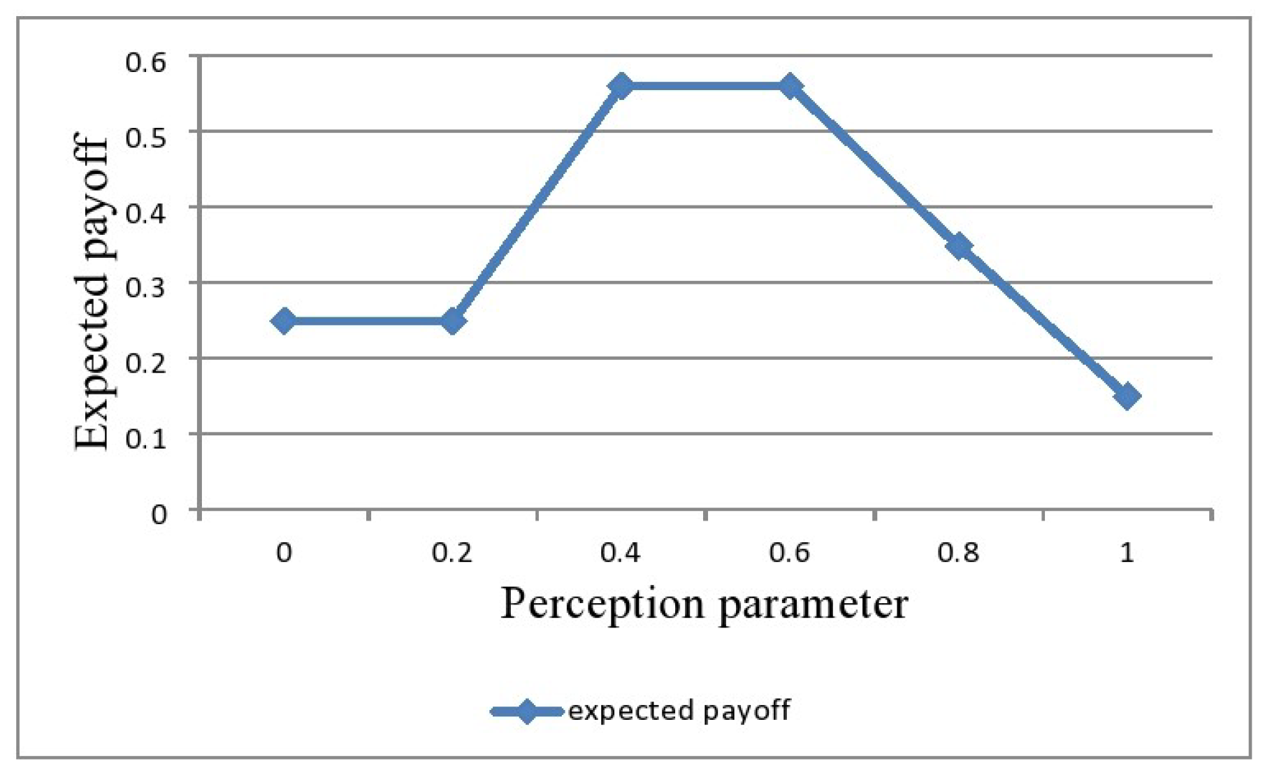
The results obtained for different values of the perception parameter are listed in Table 5.
The changes of score values of the expected payoffs for different values of the perception parameter for Player are depicted in Figure 2.
- Table 5 shows that for , we obtain the optimal strategies for the players as and . Furthermore, Player ’s aggregated expected payoff is obtained as ; . In other words, we may say that if Player ’s, i.e., the defenders’, control strategies are with a probability of 0.4518 and with a probability of 0.5482 while Player ’s, i.e., the hackers’, governing strategies are with a probability of 0.0096 and with a probability of 0.9904, and also, Player is very much optimistic toward the information, then the DMs come to an inference that the damage will be reduced with a surety from to and with a disbelief from to
- Table 5 shows that for all the values of the perception parameter This symbolizes that the crisp equivalent of the amount of gain of Player does not exceed the crisp equivalent amount of loss of Player
- Actually, the perception parameter captures the behavior of the players. From Table 5, we can see the crisp equivalent gain of Player and the crisp equivalent loss of Player both are gradually increased with the increment of the perception parameter chosen by the players. That indicates the gain value of Player is maximum when he/she is optimistic enough.
- The score values of expected payoff for Player are increased for and are decreased for This indicates that we can achieve the expected payoff for Player at the maximum level when the players are neutral in nature. This shows the importance of the role of the perception parameter in our proposed model.
- From Table 5, it is observed that the optimal strategies of the players change significantly with the changes in the perception parameter Both of the players use pure strategies only when the perception parameter lies in the interval Otherwise, the players use mixed strategies with some probabilities. For example, when Player uses strategies and with probabilities 0.4518 and 0.5482, respectively, while Player uses strategies and with probabilities 0.0096 and 0.9904, respectively. Therefore, the players have the freedom to change their strategies with the changes in to optimize their expected payoffs.
6. Comparative Analysis and Discussion
Section 6.1 and Section 6.2 justify the superiority of the rendered model in comparison with the presented methods of Bhaumik and Roy [39] and Xue et al. [45].
6.1. Comparison with Bhaumik and Roy [39]
In 2019, Bhaumik and Roy [39] introduced a special form of IIHFE in the literature along with a new aggregation operator. Aiming to consider the hesitancy of the players in terms of both their acceptance and rejection of the possible range of asymmetric information, they applied the notion of IIHFEs in matrix games. To make the solution to this problem, Bhaumik and Roy derived two interval-valued intuitionistic hesitant fuzzy programming models as follows:
and
where and are Player ’s gain floor and Player ’s loss ceiling, respectively.
Taking the defined ranking approach (assigned by Bhaumik and Roy [39]), these two problems are converted into the following linear programming models:
and
where , and are the aggregated form of the preassigned gain floor, loss ceiling, and payoffs, respectively.
Now, for the matrix the LP problems according to Problems (54) and (55) are constructed as
and
The computational results, obtained by solving Problems (56) and (57), are listed in Table 6.
Analyzing the computed results portrayed in Table 5 and Table 6, the following observations are made:
- (i)
- In our proposed method, the perception parameter plays a significant role. Table 5 shows that Player ’s gain-floor, Player ’s loss ceiling, and Player s expected payoff are changed with the changes in the perception parameter . It is observed that when the players are optimistic toward the information, i.e., when lies in players have better gain values. Hence, the players have the option to choose different parameter values to obtain better gains. However, in Bhaumik and Roy’s [39] methodology, there is no such parameter that can improve the gain of the player.
- (ii)
- In classical game theory, there is a most celebrated result that the gain floor of the winning player never exceeds the loss ceiling of the defeated player. In Theorem 2, we showed that this endures also in the IIHF environment. However, if we solve the same problem by Bhaumik and Roy’s [39] approach, we have . Table 6 shows that the gain floor is greater than the loss ceiling , which contradicts the statement of Theorem 2.
- (iii)
- (iv)
- Furthermore, it is worth noting that we need to preserve the hesitant character of IIHFEs. However, to preserve the character, if we apply mathematical operations for IIHFEs in the interval-valued intuitionistic hesitant fuzzy programming models, it yields two NLPP models instead of LP models. This phenomenon raises an essential question on the validation of Bhaumik and Roy’s [39] approach.
So, considering all these aspects, we can claim that our proposed model is superior to the existing model.
6.2. Comparison with Xue et al. [45]
This subsection provides a comparison with the celebrated methodology of matrix games discussed by Xue et al. [45]. Xue et al. [45] used hesitant fuzzy elements as the payoffs of a matrix game. To make a comparison, we promote the hesitant fuzzy payoffs assessed by Xue et al. [45] into suitable interval-valued hesitant fuzzy payoffs. The newly promoted payoff matrix is assigned in Table 7.
Now, to solve this matrix game, here, we use Problems (29) and (39). Problems (29) and (39) are two NLPPs that contain both membership and nonmembership values (i.e., the acceptance and nonacceptance of the players toward the information) of the aggregated payoffs. However, the payoffs described in Table 7 only contain the membership values. So, we switch off all nonmembership functions in Problems (29) and (39). Next, to reach the optimal values, we have to solve NLPPs (58) and (59).
and
By solving Problems (58) and (59), we obtain the optimal strategies for Players and along with their game values. In Table 8, we list both the results obtained by the proposed method and Xue et al.’s [45] method.
The following observations are recorded:
- (i)
- (ii)
- Using the optimal strategies and for Players and , respectively, if we calculate the expected payoff for Player we have The score function of this expected payoff is which gives a better value than the existing one [45].
- (iii)
- Moreover, Xue et al. [45] considered only the hesitancy of decision makers to portray the matrix game problem. However, occasionally in practical problems, DMs fail to judge the asymmetric information scenario properly. As a result, they cannot assign any precise value. Consequently, they have to choose some interval values to assign the payoffs. In that sense, delineating a matrix game problem in an intuitionistic interval-valued hesitant fuzzy environment is more realistic in the literature.
7. Conclusions
In reality, occasionally we fail to gather accurate information about an event, and we have to rely on a possible range of information. Consequently, decision makers have some hesitancy about the asymmetric information. To deal with such a situation, we actualize a matrix game problem with interval-valued intuitionistic hesitant fuzzy entries. To solve this, we derive two bi-objective interval-valued intuitionistic hesitant fuzzy programming models. It is difficult to handle such programming models traditionally. To establish the model, we define a new aggregation operator, viz., the min-max enclosure aggregation operator, for IIHFEs. Based on this operator, the ranking order of the IIHFEs is assigned. To obtain the optimal values, two interval-valued intuitionistic hesitant fuzzy programming problems are derived, which are converted into two nonlinear programming models with the perception parameters of the players.
In classical game theory, there is a most celebrated result that the gain floor of the maximizing player is always less than or equal to the loss ceiling of the minimizing player. In our discussion, we showed that this result is also valid in the IIHF environment. Here, we have explained that the perception parameter of the players plays an important role in this model. Depending on this parameter, the value of the game and the expected payoff of the conquering player are changed. To solve this problem, we have to change the fuzzy programming problem to a nonlinear programming problem. However, we were able to show that the solution obtained from the BOIIHFPMs is a noninferior solution to the solution obtained from the derived NLPPs. With a valid comparison, we showed that our executed model is superior to the existing methodologies proposed by Bhaumik and Roy [39] and Xue et al. [45].
To check the cogency of the proposed methodology, we presented an imprecise and asymmetric information scenario of hackers and of the defenders attempting to prevent cybercrime. Here, it is observed that both the gain of the winning player and the loss of the defeated player increase with the increment of the perception parameter of the player.
Besides several advantages, the proposed methodology has some limitations. One of the major limitations is that we failed to calculate the gains and losses of the players in terms of IIHFEs. Another limitation is that we generated the solution procedure by presuming the existence of a solution for matrix games in the IIHF environment. However, we cannot establish any theorems about it. Therefore, further investigation is needed in the future, which can be considered a future study of the rendered methodology.
This methodology can be applied to various decision-making problems in an IIHF environment. Moreover, in various conflicting situations, portraying the situation in terms of a possible range of acceptance and nonacceptance by the players, along with the degree of hesitancy of the players towards the information, such as various management issues, war science, psychological issues, etc., can be resolved by our proposed methodology.
Author Contributions
Conceptualization, S.K. and M.R.S.; methodology, S.K. and M.R.S.; software, S.K.; validation, S.K.; formal analysis, S.K.; investigation, M.R.S.; resources, S.K. and M.R.S.; data curation, S.K. and M.R.S.; writing—original draft preparation, S.K. and M.R.S.; writing—review and editing, M.R.S.; supervision, M.R.S. All authors have read and agreed to the published version of the manuscript.
Funding
This research received no external funding.
Data Availability Statement
Data are contained within the article.
Acknowledgments
The authors would like to acknowledge the anonymous reviewers whose invaluable comments and suggestions helped to improve the article.
Conflicts of Interest
The authors declare no conflicts of interest.
References
- Neumann, J.V.; Morgenstern, O. Theory of Games and Economic Behaviour; Princeton University Press: Princeton, NJ, USA, 1947. [Google Scholar]
- Dubois, D.; Prade, H. Fuzzy Sets and Systems: Theory and Applications; Academic Press: New York, NY, USA, 1980. [Google Scholar]
- Mi, X.; Liao, H.; Zeng, X.J.; Xu, Z. The two-person and zero-sum matrix game with probabilistic linguistic information. Inf. Sci. 2021, 570, 487–499. [Google Scholar] [CrossRef]
- Chandra, S.; Aggarwal, A. On solving matrix games with pay-offs of triangular fuzzy numbers: Certain observations and generalizations. Eur. J. Oper. Res. 2015, 246, 575–581. [Google Scholar] [CrossRef]
- Atanassov, K.T. Intuitionistic fuzzy sets. Fuzzy Sets Syst. 1986, 20, 87–96. [Google Scholar] [CrossRef]
- Li, D.F. Mathematical-programming approach to matrix games with payoffs represented by Atanassov’s interval-valued intuitionistic fuzzy sets. IEEE Trans. Fuzzy Syst. 2010, 18, 1112–1128. [Google Scholar] [CrossRef]
- Li, D.F. Decision and Game Theory in Management with Intuitionistic Fuzzy Sets; Springer: Berlin, Germany, 2014. [Google Scholar]
- Xia, M. Interval-valued intuitionistic fuzzy matrix games based on archimedean t-conorm and t-norm. Int. J. Gen. Syst. 2018, 47, 278–293. [Google Scholar] [CrossRef]
- Brikaa, M.G.; Zheng, Z.; Ammar, E.S. Resolving indeterminacy approach to solve multi-criteria zero-sum matrix games with intuitionistic fuzzy goals. Mathematics 2020, 8, 305. [Google Scholar] [CrossRef]
- Verma, T.; Kumar, A. Ambika methods for solving matrix games with Atanassov’s intuitionistic fuzzy pay-offs. IEEE Trans. Fuzzy Syst. 2018, 26, 270–283. [Google Scholar] [CrossRef]
- Verma, R.; Aggarwal, A. Matrix games with linguistic intuitionistic fuzzy payoffs: Basic results and solution methods. Artif. Intell. Rev. 2021, 54, 5127–5162. [Google Scholar] [CrossRef]
- Dong, J.Y.; Wan, S.P. Type-2 interval-valued intuitionistic fuzzy matrix game and application to energy vehicle industry development. Expert Syst. Appl. 2024, 249, 123398. [Google Scholar] [CrossRef]
- Seikh, M.R.; Karmakar, S.; Castillo, O. A novel defuzzification approach of type-2 fuzzy variable to solving matrix games: An application to plastic ban problem. Iran. J. Fuzzy Syst. 2021, 18, 155–172. [Google Scholar]
- Yang, Y.D.; Ding, X.F. A q rung orthopair fuzzy non cooperative game method for competitive strategy group decision making problems based on a hybrid dynamic experts’ weight deter-mining model. Complex Intell. Syst. 2021, 7, 3077–3092. [Google Scholar] [CrossRef]
- Bigdeli, H.; Mousazadeh, M. Analytical Hierarchy Process in modeling and solving matrix games in neutrosophic environment and its application in military problems. Mil. Sci. Tactics 2023, 19, 5–33. [Google Scholar]
- Seikh, M.R.; Dutta, S. Solution of matrix games with payoffs of single-valued trape-zoidal neutrosophic numbers. Soft Comput. 2022, 26, 921–936. [Google Scholar] [CrossRef]
- Seikh, M.R.; Dutta, S. Interval neutrosophic matrix game-based approach to counter cybersecurity issue. Granul. Comput. 2023, 8, 271–292. [Google Scholar] [CrossRef]
- Khalil, A.M.; Cao, D.; Azzam, A.; Smarandache, F.; Alharbi, W.R. Combination of the single-valued neutrosophic fuzzy set and the soft set with applications in decision-making. Symmetry 2020, 12, 1361. [Google Scholar] [CrossRef]
- Torra, V. Hesitant fuzzy sets. Int. J. Intell. Syst. 2010, 25, 529–539. [Google Scholar] [CrossRef]
- Xia, M.; Xu, Z.S. Hesitant fuzzy information aggregation in decision making. Int. J. Approx. Reason. 2011, 52, 395–407. [Google Scholar] [CrossRef]
- Xu, Z.S.; Xia, M. Distance and similarity measures for hesitant fuzzy sets. Inform. Sci. 2011, 181, 2128–2138. [Google Scholar] [CrossRef]
- Zeng, W.; Li, D.; Yin, Q. Weighted interval-valued hesitant fuzzy sets and its application in group decision making. Int. J. Fuzzy Syst. 2019, 21, 421–432. [Google Scholar] [CrossRef]
- Jana, J.; Roy, S.K. Linguistic Pythagorean hesitant fuzzy matrix game and its application in multi-criteria decision making. Appl. Intell. 2023, 53, 1–22. [Google Scholar] [CrossRef]
- Seikh, M.R.; Karmakar, S.; Xia, M. Solving matrix games with hesitant fuzzy pay-offs. Iran. J. Fuzzy Syst. 2020, 17, 25–40. [Google Scholar]
- Yang, Z.; Song, Y. Matrix game with payoffs represented by triangular dual hesitant fuzzy numbers. Int. J. Comput. Commun. Control 2020, 15, 3854. [Google Scholar] [CrossRef]
- Naqvi, D.R.; Sachdev, G.; Ahmad, I. Matrix games involving interval-valued hesitant fuzzy linguistic sets and its application to electric vehicles. J. Intell. Fuzzy Syst. 2023, 44, 5085–5105. [Google Scholar] [CrossRef]
- Zhang, Z. Interval-valued intuitionistic hesitant fuzzy aggregation operators and their application in group decision-making. J. Appl. Math. 2013, 2013, 670285. [Google Scholar] [CrossRef]
- Broumi, S.; Smarandache, F. New operations over interval-valued intuitionistic hesi-tant fuzzy set. Math. Stat. 2014, 2, 62–71. [Google Scholar] [CrossRef]
- Joshi, D.K.; Kumar, S. Interval-valued intuitionistic hesitant fuzzy choquet integral based TOPSIS method for multi-criteria group decision making. Eur. J. Oper. Res. 2016, 248, 183–191. [Google Scholar] [CrossRef]
- Yuan, J.; Li, C.; Xu, F.; Sun, B.; Li, W. A group decision making approach in inter-val-valued intuitionistic fuzzy environment with confidence levels. J. Intell. Fuzzy Syst. 2016, 31, 1909–1919. [Google Scholar] [CrossRef]
- Joshi, D.K.; Kumar, S. Entropy of interval-valued intuitionistic hesitant fuzzy set and its application to group decision making problems. Granul. Comput. 2018, 3, 367–381. [Google Scholar] [CrossRef]
- Narayanamoorthy, S.; Geetha, S.; Rakkiyappan, R.; Joo, Y.H. Interval-valued intuitionistic hesitant fuzzy entropy based VIKOR method for industrial robots selection. Expert Syst. Appl. 2019, 121, 28–37. [Google Scholar] [CrossRef]
- De, A.; Das, S.; Kar, S. Multiple attribute decision making based on probabilistic inter-val-valued intuitionistic hesitant fuzzy set and extended TOPSIS method. J. Intell. Fuzzy Syst. 2019, 37, 5229–5248. [Google Scholar] [CrossRef]
- Du, K.; Fan, R.; Wang, Y.; Wang, D.; Qian, R.; Zhu, B. A data-driven group emergency decision-making method based on interval-valued intuitionistic hesitant fuzzy sets and its application in COVID-19 pandemic. Appl. Soft Comput. 2023, 139, 110213. [Google Scholar] [CrossRef]
- Bhaumik, A.; Roy, S.K.; Weber, G.W. Hesitant interval-valued intuitionistic fuzzy-linguistic term set approach in prisoners’ dilemma game theory using TOPSIS: A case study on hu-man-trafficking. Cent. Eur. J. Oper. Res. 2020, 28, 797–816. [Google Scholar] [CrossRef]
- Zhai, Y.; Xu, Z.; Liao, H. Measures of probabilistic interval-valued intuitionistic hesitant fuzzy sets and the application in reducing excessive medical examination. IEEE Trans. Fuzzy Syst. 2018, 26, 1651–1670. [Google Scholar] [CrossRef]
- Zhang, L.; Tang, J.; Meng, F. An approach to decision making with interval-valued in-tuitionistic hesitant fuzzy information based on the 2-additive shapley function. Informatica 2018, 29, 157–185. [Google Scholar] [CrossRef]
- Zhang, G.; Zhou, S.; Xia, X.; Yuksel, S.; Bas, H.; Dincer, H. Strategic mapping of youth unemployment with interval valued intuitionistic hesitant fuzzy DEMATEL based on 2-tuple linguistic values. IEEE Access 2020, 8, 25706–25721. [Google Scholar] [CrossRef]
- Bhaumik, A.; Roy, S.K. Intuitionistic interval-valued hesitant fuzzy matrix games with a new aggregation operator for solving management problem. Granul. Comput. 2021, 6, 359–375. [Google Scholar] [CrossRef]
- Xu, Z.; Gou, X. An overview of interval-valued intuitionistic fuzzy information aggrega-tions and applications. Granul. Comput. 2017, 2, 13–39. [Google Scholar] [CrossRef]
- Chen, N.; Xu, Z.S. Properties of interval-valued hesitant fuzzy sets. J. Telligent Fuzzy Syst. 2014, 27, 143–158. [Google Scholar] [CrossRef]
- Xu, Z.S. Intuitionistic fuzzy aggregation operator. IEEE Trans. Fuzzy Syst. 2007, 15, 1179–1187. [Google Scholar]
- Ishibuchi, H.; Tanaka, H. Multiobjective programming in optimization of the interval objective function. Eur. J. Oper. Res. 1990, 48, 219–225. [Google Scholar] [CrossRef]
- National Crime Records Bureau. 2020. Available online: https://ncrb.gov.in/en/Crime-in-India-2020 (accessed on 27 June 2023).
- Xue, W.; Xu, Z.; Zeng, X.J. Solving matrix games based on Ambika method with hesitant fuzzy information and its application in the counter-terrorism issue. Appl. Intell. 2021, 51, 1227–1243. [Google Scholar] [CrossRef]
Figure 1.
State-wise reported number of cybercrimes in last three years.
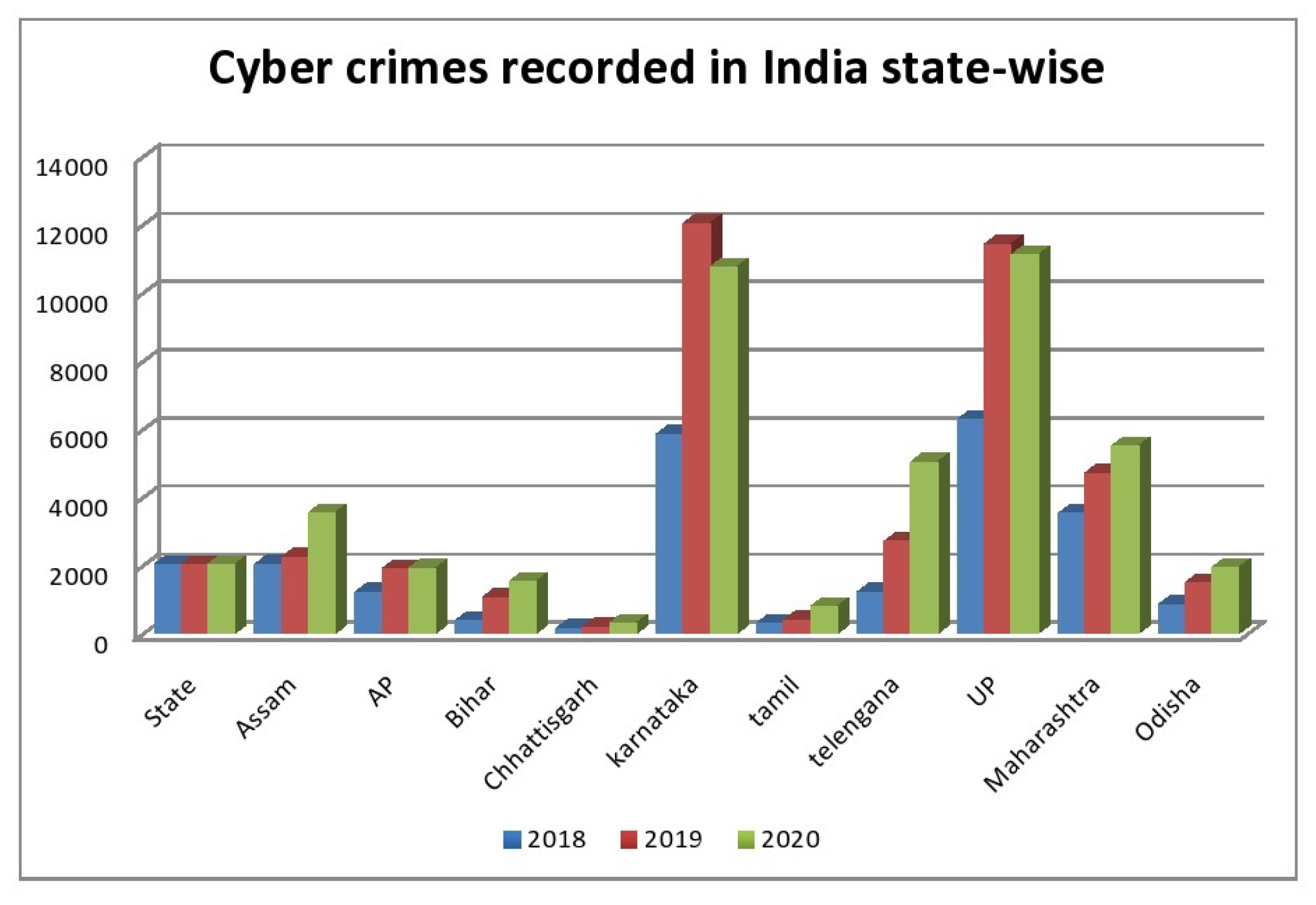
Figure 2.
Change of expected payoffs with respect to the perception parameter .

Table 1.
Payoff matrix assigned by DM 1.
| Strategies | ||
|---|---|---|
Table 2.
Payoff matrix assigned by DM 2.
| Strategies | ||
|---|---|---|
Table 3.
Payoff matrix assigned by DM 3.
| Strategies | ||
|---|---|---|
Table 4.
Aggregated value of the decisions.
(p = 1, 2; q = 1, 2) | Aggregated IIHFEs |
|---|---|
| 〈[0.6858,0.7861], [0.7079,0.8771], [0.7025,0.8263], [0.7234,0.9002], [0.6858,0.8038], [0.7079,0.8873]; [0.5145,0.6284], [0.5145,0.6684], [0.5145,0.6437], [0.5145,0.6846]〉 | |
| 〈[0.4608,0.7358], [0.6104,0.7358], [0.5941,0.7544], [0.5891,0.7544], [0.4608,0.7576], [0.6104,0.7576], [0.5941,0.7747], [0.5941,0.7747]; [0.5365,0.6089], [0.5123,0.7309], [0.4969,0.6089], [0.4745,0.7309]〉 | |
| 〈[0.3304,0.4565], [0.3304,0.4854], [0.3154,0.4565]; [0.4573,0.5936], [0.4573,0.6069], [0.4431,0.5936], [0.4431,0.6069]〉 | |
| 〈[0.6157,0.7160], [0.6157,0.7000], [0.6309,0.7160], [0.6356,0.7359], [0.6356,0.7211], [0.6500,0.7359]; [0.3342,0.4437], [0.3342,0.4573]〉 |
Table 5.
Result table.
| 0 | (0,1) | 0.5063 | (1,0) | 0.5063 | 0.2492 | |
| 0.2 | (0,1) | 0.5250 | (1,0) | 0.5250 | 0.2492 | |
| 0.4 | (0,1) | 0.5337 | (0,1) | 0.5337 | 0.5601 | |
| 0.6 | (0,1) | 0.5883 | (0,1) | 0.5883 | 0.5601 | |
| 0.8 | (0.4518,0.5482) | 0.6301 | (0.0096,0.9904) | 0.6339 | 0.3481 | |
| 1 | (0.4898,0.5102) | 0.6510 | (0.1336,0.8664) | 0.6682 | 0.1494 |
Table 6.
Results obtained by Bhaumik and Roy’s [39] method.
Table 6.
Results obtained by Bhaumik and Roy’s [39] method.
| (0,1) | 0.5009 | (0.2949,0.7051) | 0.0881 | 0.1482 |
Table 7.
Payoff matrix in tabular form.
| Strategy | ||||
|---|---|---|---|---|
Table 8.
Comparative results of proposed method and Xue et al.’s [45] method.
Disclaimer/Publisher’s Note: The statements, opinions and data contained in all publications are solely those of the individual author(s) and contributor(s) and not of MDPI and/or the editor(s). MDPI and/or the editor(s) disclaim responsibility for any injury to people or property resulting from any ideas, methods, instructions or products referred to in the content. |
© 2024 by the authors. Licensee MDPI, Basel, Switzerland. This article is an open access article distributed under the terms and conditions of the Creative Commons Attribution (CC BY) license (https://creativecommons.org/licenses/by/4.0/).
Share and Cite
MDPI and ACS Style
Karmakar, S.; Seikh, M.R. A Nonlinear Programming Approach to Solving Interval-Valued Intuitionistic Hesitant Noncooperative Fuzzy Matrix Games. Symmetry 2024, 16, 573. https://doi.org/10.3390/sym16050573
AMA Style
Karmakar S, Seikh MR. A Nonlinear Programming Approach to Solving Interval-Valued Intuitionistic Hesitant Noncooperative Fuzzy Matrix Games. Symmetry. 2024; 16(5):573. https://doi.org/10.3390/sym16050573
Chicago/Turabian StyleKarmakar, Shuvasree, and Mijanur Rahaman Seikh. 2024. "A Nonlinear Programming Approach to Solving Interval-Valued Intuitionistic Hesitant Noncooperative Fuzzy Matrix Games" Symmetry 16, no. 5: 573. https://doi.org/10.3390/sym16050573
Note that from the first issue of 2016, this journal uses article numbers instead of page numbers. See further details here.