Article

Exploring Endogenous Processes in Water Supply Systems: Insights from Statistical Methods and δ18O Analysis

by
Nikolina Novotni-Horčička
1,
Tamara Marković
2,*,
Ivan Kovač
3 and
Igor Karlović
2
1
Varkom d.o.o., 42000 Varaždin, Croatia
2
Croatian Geological Survey, 10000 Zagreb, Croatia
3
Faculty of Geotechnical Engineering, University of Zagreb, 42000 Varaždin, Croatia
*
Author to whom correspondence should be addressed.
Water 2024, 16(10), 1425; https://doi.org/10.3390/w16101425
Submission received: 19 March 2024 / Revised: 6 May 2024 / Accepted: 10 May 2024 / Published: 16 May 2024
(This article belongs to the Section Urban Water Management)

Abstract

:
Water used for water supply undergoes numerous changes that affect its composition prior to entering the water supply system (WSS). Once it enters the WSS, it is subject to numerous influences altering its physical and chemical composition, redox potential, and microbial quality. Observations of water quality parameters at different locations within the WSS indicate that it is justified to assume that these processes take place from the source to the end user. In this study, we used the results of routine everyday analyses (EC, T, pH, ORP, chloride, nitrate, nitrite, ammonium, and bacteria) supplemented by experimental data from a one-year sampling campaign assessing the main cations and anions and stable isotopes δ2H and δ18O. Through these data, the statistical significance of the differences between the concentrations of the basic water quality parameters among different WSS locations was determined, together with the water retention time in the system. The results indicate minor changes in water chemical composition within the observed WSS, remaining below the prescribed Maximum Contaminant Level (MCL) for human consumption. However, factors such as water retention time, CaCO3 deposition, pH fluctuations, and bacterial growth may influence its suitability, which necessitates further investigation into potential risks affecting water quality.

1. Introduction

Water entering the water supply system (WSS) must be in accordance with the prescribed requirements for human consumption [1,2]. Before reaching the WSS, it undergoes disinfection processes and/or other conditioning procedures, depending on the quality of the water at the sources. However, the system itself is subjected to the influence of various processes that may affect its regulatory compliance, as well as organoleptic acceptability by consumers. The water supply system is a complex network consisting of pipes with different diameters and lengths, along with tanks, pumps, valves, and other plumbing devices made of various materials, all of which can have an impact on the processes within the system. The potentially occurring process is the formation of biofilms due to microbial growth in the presence of nutrients, such as natural organic matter, iron, nitrogen, phosphorus, manganese, sulfates, and humic substances, that are originally present or have entered the system after processing [3]. Additional processes include the formation and release of deposits in pipes, corrosion, and the formation of harmful disinfection byproducts due to interaction between the disinfectant and organic matter in water, etc. [4,5,6,7,8,9]. All these processes could have a significant impact on water quality and acceptability [4,5,6,7].
The water supply system is dynamic, as hydraulic conditions fluctuate continuously over a 24 h period due to consumption needs and malfunctions within the system (pipe burst, maintenance activities, etc.). This dynamic nature leads to changes in the water flow direction, pressure, and temperature, which can influence the water retention time within the system, cause changes in pH, influence the solubility of metals present in the system, etc. [8,9].
Water suppliers are obligated to control the quality of delivered water to consumers. Water quality monitoring is carried out within the framework of conducting basic and extended chemical and microbiological analyses on a daily, weekly, and monthly basis depending on the number of consumers and amount of water pumped. By systematically collecting this data, water suppliers gain insights into the water quality within their system, allowing them to improve guidelines for managing the WSS [10,11]. The collected data can be used as a base for statistical analysis in order to predict whether water quality will deteriorate in the near or distant future [12,13,14,15]. The stable water isotopes δ2H and δ18O serve as very useful tools in the analysis of the water cycle, providing essential information about water retention time (residence time), identification of chemical processes, etc. [16,17,18,19,20]. According to the US EPA [21], water retention time is the main factor affecting the deterioration of water quality in WSSs. It often happens that, due to less consumption or over-dimensioning of the system for fire flow requirements, water stays in pipes or reservoirs for a longer time, which leads to a decrease in disinfectant concentration. This further facilitates microbial growth, changes in pH levels, particularly during warmer months due to increases in water temperature, and various reactions between materials or sediments. Methods for determining water retention time in WSSs include chemical tracers, mathematical models, or their combined use, each with its own set of advantages and disadvantages [22,23]. Recently, naturally occurring radioactive and stable isotopes in water have been utilized for the determination of the water retention time in distribution systems [24].
This paper explores the application of δ18O and statistical data processing on selected chemical parameters within a small part of the water supply network managed by Varkom Inc., Croatia. The objectives of the study were the following: (i) to characterize the water from the source to the tap by analyzing hydrochemical parameters; (ii) to statistically analyze selected water quality parameters: chloride, nitrate, pH, electrical conductivity (EC) and temperature (T) over a two-year period, aiming to detect any significant changes that would potentially impact the compliance of the drinking water standards; (iii) to verify the reliability of basic statistical analysis results through geochemical modeling; (iv) to calculate the water retention time in the WSS by using δ18O and an algorithm based on technical WSS information, and compare the obtained results. All this work is carried out to ensure sustainable management of the WSS, not only within the studied system but also to validate its applicability for WSSs worldwide.

2. Materials and Methods
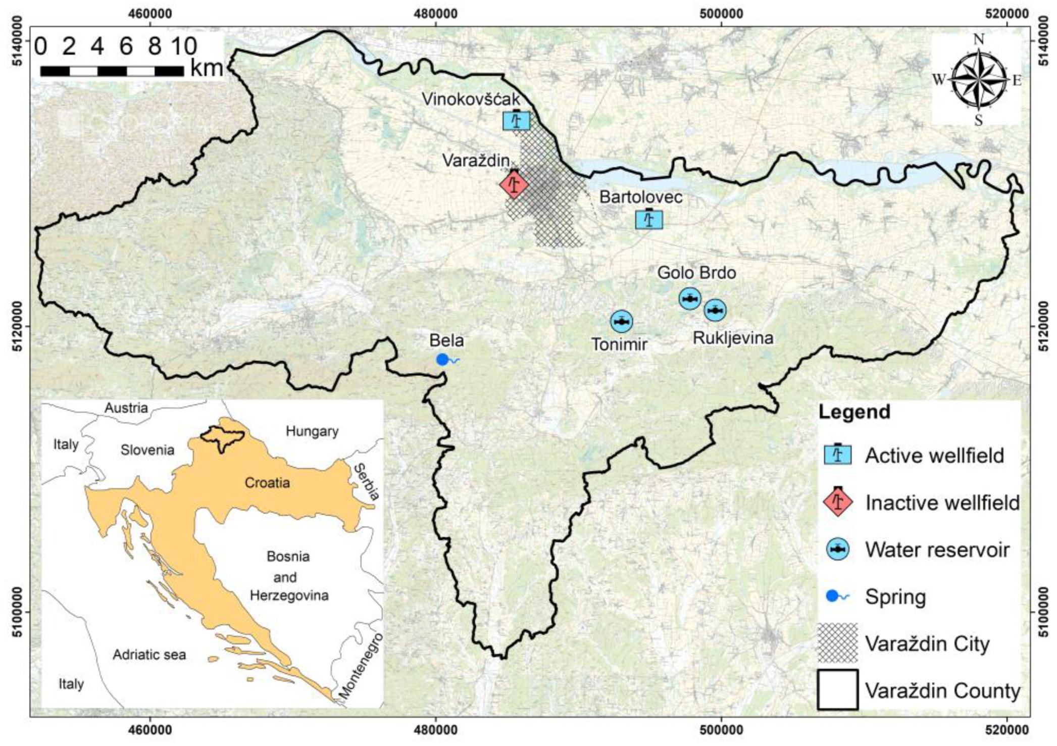
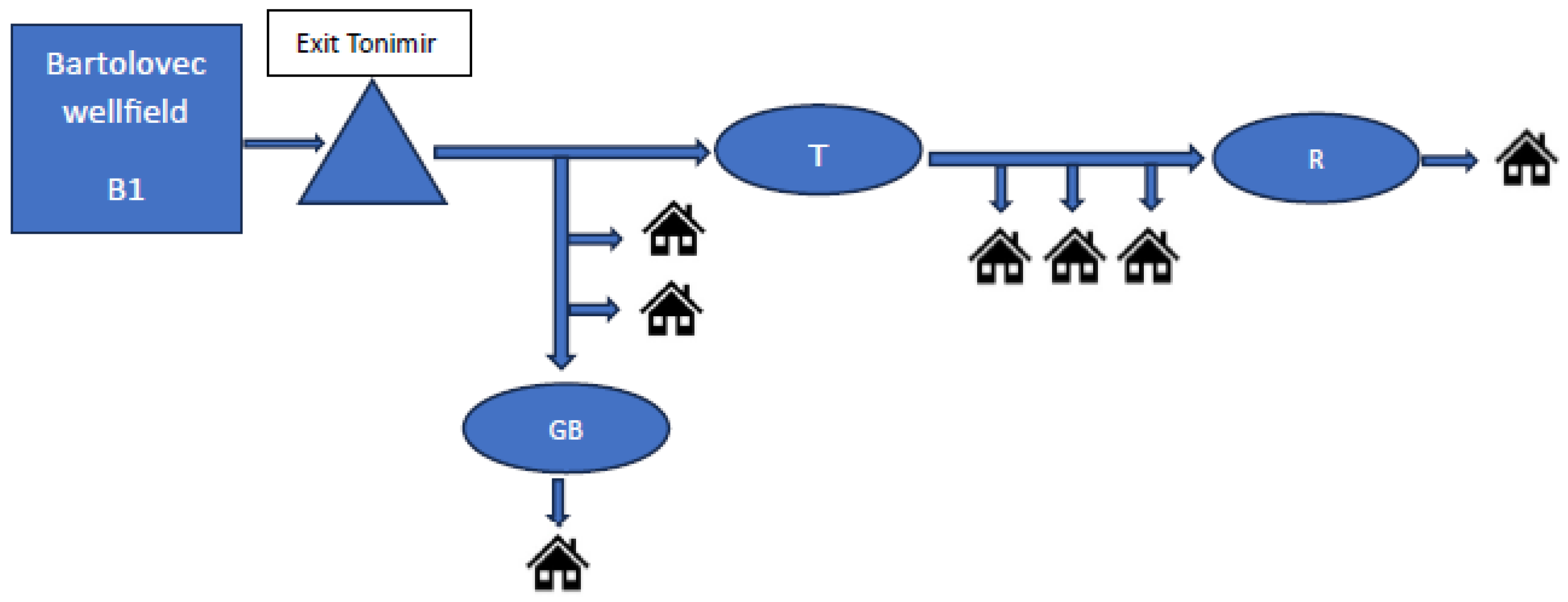
2.1. Research Area

This research focused on a small segment of the WSS operated by Varkom Inc. in Varaždin County, northwestern Croatia (Figure 1). The whole WSS spans approximately 1600 km, comprising 20 reservoirs with a total volume of 19,500 m3, and supplies about 120,000 inhabitants [25]. Generally, there is no water treatment (except for one well that is filtered through activated carbon, but it is not situated in the study area).
The entire WSS is mixed and very complex, drawing water from three groundwater sources (Bartolovec and Vinokovšćak wellfields, and Bela spring). For this study, a small segment of the WSS was selected due to its well-defined traceability, allowing tracking of the water flow from the pumped well through pipelines to the reservoir, without mixing water from other wells. This approach enables us to monitor changes in chemical parameters throughout the distribution. Specifically, this study centered around well B-1 at the Bartolovec wellfield, from which water is drawn and sent through pipelines to the Tonimir (T)and Golo Brdo (GB) water reservoirs, which have volumes of 500 m3 and 100 m3. The water from the Tonimir reservoir is directed for consumption, while a flow rate of 4.2 L/s fills the 100 m3 large Rukljevina (R) water reservoir (Figure 2).

2.2. Water Sampling and Analysis

Water samples were taken from well B-1 and reservoirs T, GB, and R by two different companies employing different sampling frequencies.
The first data set is a part of the water sampling campaigns from well B-1 and reservoirs T, GB, and R as part of the operational monitoring of the Varkom Inc. supplier from Varaždin, Croatia. Samples were collected in accordance with HRN ISO 5667-5:2011: Water quality—Sampling—Part 5: Guidance on sampling of drinking water from treatment works and piped distribution systems (ISO 5667-5:2006) and analyzed in its own laboratory. The dynamics of the sampling were once a week throughout 2021 and 2022. The monitored water quality parameters include pH, electrical conductivity (EC), chloride (Cl), and nitrate (NO3). These parameters were chosen because they are part of regular analysis and show certain spatial and temporal fluctuations. During this monitoring, additional parameters, such as NO2, NH4+, temperature, turbidity, free residual chlorine, and microbiological indicators, were also measured. However, they are not included in this study due to the following specific reasons: nitrite (NO2) and ammonium (NH4+) are consistently below detection limits, while the remaining parameters depend on external influences. In addition, heavy metals were not considered because of the following: they are not included in the everyday routine analysis and concentrations are very low, mostly below the detection limit in wells and WSS waters. The pH and EC parameters were measured using a multimeter (Multimeter HQ40d, HACH, Ames, IA, USA); chlorides were determined by titration (Stand. Meth. 22nd Ed., 4500-Cl-B), and nitrates were determined spectrophotometrically (St. Meth. 22nd Ed., 4500-NO3-B) on a UV-VIS spectrophotometer (Camspec, M509T, Leeds, UK). The precision and accuracy of analytical methods were below 10%, as determined by repeated measurement of standard solutions of known concentration (CertiPUR, Merck, VWR Chemicals, Radnor, PA, USA).
The second data set was obtained from three sampling campaigns in July and November 2022 (well B-1 and reservoir T) and February 2023 (well B-1 and reservoirs T, R, and GB) performed by the Hydrochemical Laboratory of Croatian Geological Survey, Zagreb, Croatia within the scopes of the TRANITAL and WATSON projects. Prior to sampling, pH, EC, T, dissolved oxygen (DO), and redox potential (ORP) were measured using a WTW multimeter. Concentrations of basic anions and cations were analyzed on Ion Chromatograph Dionex ICS 6000, while alkalinity was determined by titration with 1.6 N H2SO4 with phenolphthalein and bromocresol green-methyl indicators, and then converted into equivalent concentrations of HCO3. The precision of the measurements was determined based on the charge balance of the main ions, as quantified by Ion Balance Error (IBE), which was less than 5%.
Ratios of the stable isotopes δ18O and δ2H were determined using a Picarro L2130i device (Santa Clara, CA, USA) using CRDS (Cavity Ring-Down Spectroscopy) technology [25], and the results were expressed according to the international standard. USGS standards were used to control measurements, which were periodically checked according to the IAEA international standards: Vienna Standard Mean Ocean Water 2 (VSMOW2) and Standard Light Antarctic Precipitation 2 (SLAP2). For δ18O, the measurement precision was ±0.2‰, while for δ2H, it was ±0.9‰.

2.3. Data Analysis

For each parameter at every location, the number of data points (n), average concentration x ¯ , corresponding variance σ 2 , and its estimate s 2 were determined:
s i 2 = n i n i 1 σ i 2
In order to determine the statistical significance of the difference between the concentrations at the locations Li and Lj, it is necessary to apply the t-test:
t = x ¯ i x ¯ j s d
whereby:
s d 2 = n i 1 s i 2 + n j 1 s j 2 n i + n j 2 · n i + n j n i · n j
The obtained t-value was compared with the critical value t α , which was determined for a significance level of 5% and based on the number of degrees of freedom:
k = n i + n j 2
Statistical data processing was conducted using the MS Excel tool.

Hypothesis

It is clear from expression (2) that the t-value is proportional to the difference between the average concentrations at locations Li and Lj. If the t-value is less than the critical one, the null hypothesis (H0) is accepted, indicating that the observed difference is not statistically significant. Otherwise, the alternative hypothesis (H1) is accepted:
t t α             H 0 :       x ¯ i = x ¯ j
t > t α             H 1 :       x ¯ i x ¯ j
If the t-value is greater than the critical one, the difference between the average concentrations is considered statistically significant, which indicates an endogenous process in the water between locations Li and Lj within the water supply system.

2.4. Water Retention Time (Water Age)

The calculation of water retention time of water in the Tonimir reservoir was performed by using δ18O measurements in well and reservoirs. The calculation utilized a simplified model by [25], which was applied to estimate the residence time of water in the ground:
t = 1 / 2   π × 1   / b / a 2 1   y e a r s
where t is the estimated residence time, b is the maximal amplitude of the groundwater isotopic data, and a is the maximal amplitude of the precipitation isotopic data over several years. This formula was adapted for our specific context, where t represents the estimated retention time of water in the system, b is the maximal amplitude of the water in the reservoir, and a is the maximal amplitude of the water isotopic data from well B-1 over two-year monthly measurements. Water retention time in two other reservoirs was not calculated due to stable isotopes being measured only once. To verify the calculated result, water retention time was estimated using an algorithm that takes into account input parameters such as the diameters and length of pipes, reservoir dimensions, and water flux within the pipes.
The PHREEQC version 3 software was used to determine saturation indices and CO2 pressure as calculations of carbonate balance within the reservoir system [26].

3. Results and Discussion

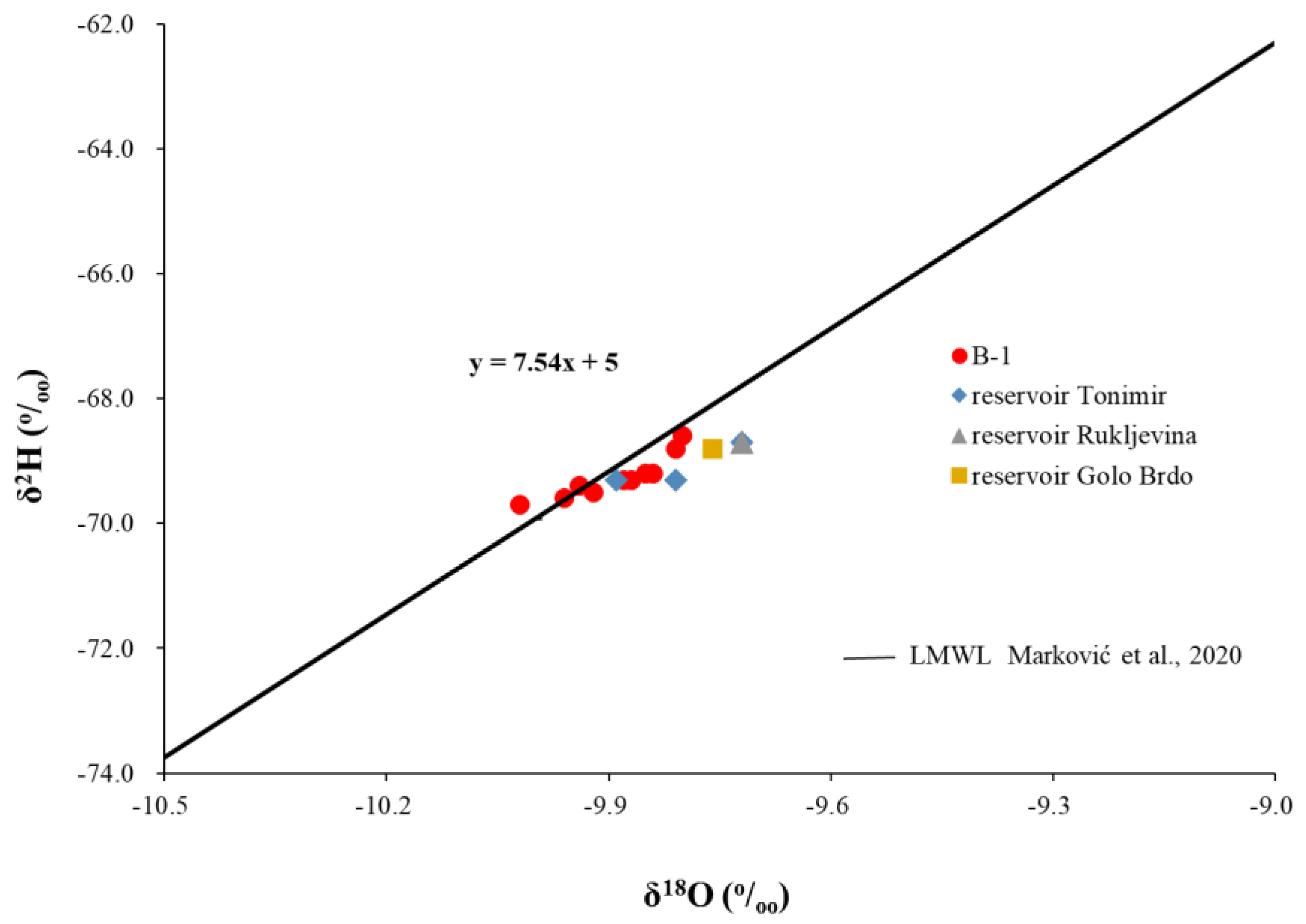
3.1. Hydrochemical Characteristics of Sampled Water

From Table 1 and Table 2, it is observed across all sampling campaigns that the EC values are higher in the well water than in reservoirs, ranging from 584 to 680 µS/cm for wells and from 481 to 674 µS/cm for reservoirs. pH values displayed oscillations in well and reservoir waters, with the highest oscillation noted during the year 2022. Furthermore, pH values are higher in reservoir waters than in well waters. Both average Cl and NO3 concentrations are similar in 2021 and 2022. However, oscillations were observed in minimum and maximum concentrations during this period. By comparing both years, a slight increase in the pH value at all locations and a decrease in chloride and nitrate concentrations, and, consequently, electrical conductivity, at all locations were observed. DO concentrations and ORP were lower in well water in comparison to reservoir waters. Additionally, it is observed that the ORP is the highest in T reservoirs (first in the row after chlorination) and gradually decreases in more distant reservoirs (Table 2). Samples taken from wells represent raw water, meaning that DO concentrations and ORP reflect the natural status of the water within the aquifer. At the T reservoir, water is coming directly after chlorination, so the ORP is higher here than in reservoirs GB and R. This suggests that water travels faster towards reservoir T, followed by reservoir GB, and takes the longest time to reach reservoir R. During this transit, chlorine degassing occurs, leading to a decrease in ORP. The alkalinity (HCO3) was the highest in the well water, while the lowest concentration was measured in the most distant reservoirs (R and GB) from the well (Table 2).
According to major ion composition, both reservoir waters and well B-1 waters have the same hydrochemical type, characterized as CaMg-HCO3, without pronounced differences on the Piper diagram (Figure 3).
However, when observing the relationship between the pH, logpCO2 pressure, and calcium saturation index (SIcalcite), differences are noticed (Figure 4a,b). The well water exhibits a lower pH value and SIcalcite, but higher logpCO2. On the other hand, reservoir waters display higher values of pH and SIcalcite, but lower logpCO2 (Figure 4b). In addition, it was observed that in the reservoir farthest from the well, where water retention time is the longest, the pH tended to be higher (Figure 4a).
Given that reservoirs, in a geochemical context, represent open systems where the exchange of gasses between air and water occurs (as there is space above the water filled with air), groundwater from well B-1 is oversaturated with CO2. When well water reaches reservoirs, degassing of CO2 occurs and, as a consequence, the shifting of the carbonate mass balance towards the left side of the well-known equation occurs:
CO2(g) + H2O + CaCO3 ↔ Ca2+ + 2HCO3
With a calcium saturation index above 0, precipitation of calcium in the water is induced, leading to the formation of a calcium crust on the water surface in reservoirs. This reaction results in a decrease in alkalinity, as well as an increase in pH due to precipitation of calcium carbonate, which further contributes to the decrease in EC.
All measured values for δ2H and δ18O in reservoirs and wells indicate that the water has a meteoric origin (Figure 5), as they are scattered around the local meteoric water line (LMWL) of the study area [20]. Values of isotopes ranged from −9.98 (well B-1) to −9.72‰ (reservoirs T and R) for δ18O, and from −69.3 (reservoir T) to 68.6‰ (well B-1) for δ2H. According to the measured δ2H and δ18O values in the water from reservoirs, there was no evaporation effect during the sampling campaigns, indicating a short water retention time. Consequently, the retention time is not long enough to be affected by seasonal temperature changes, which could potentially affect water temperature in reservoirs and thus isotope fractionation.

3.2. Water Retention Time in the Tonimir Reservoir

According to Equation (7), water retention time in the Tonimir reservoir is estimated to be approximately 17 h using the stable isotope δ18O. Employing the methodology that takes into account the technical characteristics of the water supply system yields a similar estimate of around 16.2 h. The consistency between the results obtained from both methods indicates that δ18O could be a useful and reliable tool to gather information about the system, especially when WSS managers encounter situations where their understanding of the system’s operation is limited.

3.3. Findings of Statistical Data Processing

Using the data from Table 1, the statistical significance of the differences in concentrations of the measured indicators was determined by comparing the locations on the network (reservoirs T, GB, and R) with the data at the starting sampling point—well B-1 at the wellfield. The calculated t-values were then compared with tα, which, for the given number of data points, is 1.984 [27]. The results of these comparisons are summarized in Table 3a,b.
Consistent with hypotheses (5) and (6), the obtained results show that, in 2021, negative t-values increased with the distance from well B-1 for pH and NO3, with significant difference observed for NO3 in water reservoirs GB and R (Table 3a). For EC, positive t-values increased with distance from well B-1 but did not demonstrate a significant difference in chloride concentration.
In 2022, the analysis revealed an increase in negative t-values with distance for pH and NO3, whereas, for EC, it decreased in the more distant water reservoirs GB and R (Table 3b). Conversely, the t-value for Cl is positive and it is increasing. For the parameters pH, Cl, and NO3, a significant difference was observed between the water samples from B-1 and reservoirs GB and R, as all t-values are greater than the critical tα.
In both monitored years, differences were noted in the t-values for pH, but these differences were more significant for 2022, as a result of CO2 degassing from water, as explained in Section 3.1. However, since reservoir systems are very dynamic (filling with fresh water and undergoing aeration during regular maintenance), the pH of water within reservoirs would not reach the critical value for human consumption of 9.5. Hypothetically, considering reservoir T as an example, if the reservoir were sealed, without inflow or outflow occurring, the pH would gradually increase until reaching an equilibrium between CO2 in the water and air.
The significant decrease in chloride could be attributed to chlorine degassing. Even ORP is decreasing and, in WSSs, ORP and chlorine concentrations are very well connected [28]. However, looking at the mean, minimum, and maximum measured values and considering the measuring error of ±10%, it is evident that all of them fall within a similar range. The same issue appears when analyzing nitrate concentrations. While bacteria from biofilms in pipes could potentially reduce nitrate into nitrite or ammonium. All measured values for these two parameters are consistently below the detection limit, which is <0.01 mg/L. In these two cases, statistical data processing led us to unreliable conclusions.
Despite the occurrence of precipitation of calcium carbonate and degassing of chlorine, their impact on reservoir waters is not significant.

4. Conclusions

In this paper, we elaborated on the advantages and disadvantages of employing δ18O isotopes, geochemical modeling, and statistical data processing to determine water retention time in WSSs, and investigated how retention time influences water quality within the system and the significance of the processes that are occurring. The major findings are the following:
  • The application of statistical data processing indicated the significance of certain changes within the WSS. However, the results of statistical processing should not be taken easily, because they can lead to wrong conclusions.
  • Electrical conductivity decreases with increasing distance from the well due to the precipitation of calcium carbonate.
  • In the example of the Tonimir reservoir, the water retention time is not long enough that it could deteriorate the water quality in the system.
  • pH change is occurring. However, it will never reach MCL, which is pH 9.5, due to the dynamic status of WSSs—short water retention time.
  • Stable isotopes have proven to be useful for calculating water retention time in the system, and they can be a useful complement to the management of WSSs.

Author Contributions

Conceptualization, N.N.-H., I.K. (Ivan Kovač), and T.M.; methodology, T.M.; software, I.K. (Ivan Kovač); formal analysis, N.N.-H. and T.M.; investigation N.N.-H., I.K. (Igor Karlović), and T.M.; writing—original draft preparation, N.N.-H.; writing—review and editing, T.M., I.K. (Igor Karlović), and I.K. (Ivan Kovač). All authors have read and agreed to the published version of the manuscript.

Funding

This research was funded by the Croatian Scientific Foundation (HRZZ) under grant number HRZZ-IP-2016-06-5365.

Data Availability Statement

Data sharing is not applicable.

Acknowledgments

The authors would like to thank the Varaždin Utility Company (VARKOM) and Robert Rutić, for their great help during sampling campaigns, and Davor Soldatek, for calculating water retention time within the WSS using a mathematical algorithm and helping us to verify our calculation.

Conflicts of Interest

The authors declare no conflicts of interest. The funders had no role in the design of the study; in the collection, analyses, or interpretation of data; in the writing of the manuscript; or in the decision to publish the results.

References

  1. Directive (EU) 2020/2184 of the European Parliament and of the Council of 16 December 2020 on the Quality of Water Intended for Human Consumption (Recast) (Text with EEA Relevance). Available online: http://data.europa.eu/eli/dir/2020/2184/oj (accessed on 7 November 2023).
  2. OG 30/2023, (Zakon o Vodi za Ljudsku Potrošnju Narodne Novine 30 2023). Available online: https://narodne-novine.nn.hr/clanci/sluzbeni/2023_03_30_509.html (accessed on 18 March 2024).
  3. Chu, S.; Xian, L.; Lai, C.; Yang, W.; Wang, J.; Long, M.; Ouyang, J.; Liao, D.; Zeng, S. Migration and risks of potentially toxic elements from sewage sludge applied to acid forest soil. J. For. Res. 2023, 34, 2011–2026. [Google Scholar] [CrossRef]
  4. Prest, E.I.; Hammes, F.; Van Loosdrecht, M.C.; Vrouwenvelder, J.S. Biological stability of drinking water: Controlling factors, methods, and challenges. Front. Microbiol. 2016, 7, 45. [Google Scholar] [CrossRef] [PubMed]
  5. Fish, K.; Osborn, A.M.; Boxall, J.B. Biofilm structures (EPS and bacterial communities) in drinking water distribution systems are conditioned by hydraulics and influence discolouration. Sci. Total Environ. 2017, 593–594, 571–580. [Google Scholar] [CrossRef]
  6. Ainsworth, R. Save Piped Water: Managing Microbial Water Quality in Piped Distribution Systems; WHO: Geneva, Switzerland; IWA: London, UK, 2004. [Google Scholar]
  7. Liu, J.; Chen, H.; Huang, Q.; Lou, L.; Hu, B.; Endalkachew, S.D.; Mallikarjuna, N.; Shan, Y.; Zhou, X. Characteristics of pipe-scale in the pipes of an urban drinking water distribution system in eastern China. Water Sci. Technol. Water Supply 2015, 16, 715–726. [Google Scholar] [CrossRef]
  8. Boulay, N.; Edwards, M. Role of temperature, chlorine, and organic matter in copper corrosion by-product release in soft water. Water Res. 2001, 35, 683–690. [Google Scholar] [CrossRef] [PubMed]
  9. Gonzalez, S.; Lopez-Roldan, R.; Cortina, J.-L. Presence of metals in drinking water distribution networks due to pipe material leaching: A review. Toxicol. Environ. Chem. 2013, 95, 870–889. [Google Scholar] [CrossRef]
  10. OG, 64/2023 Ordinance on (Pravilnik o Parametrima Sukladnosti, Metodama Analiza i Monitorintima Vode Namijenjene za Ljudsku Potrošnju, Narodne Novine 64 2023). Available online: https://narodne-novine.nn.hr/clanci/sluzbeni/2023_06_64_1057.html (accessed on 18 March 2024).
  11. OG, 88/2023 Ordinance on (Pravilnik o Sanitarno-Tehničkim i Higijenskim te Drugim Uvjetima Koje Moraju Ispunjavati Građevine za Vodoopskrbu i Poslovanje u Njima, Narodne Novine 88 2023). Available online: https://www.zakon.hr/cms.htm?id=57670 (accessed on 18 March 2024).
  12. Nemčić-Jurec, J.; Ruk, D.; Oreščanin, V.; Kovač, I.; Ujević Bošnjak, M.; Kinsela, A.S. Groundwater contamination in public water supply wells: Risk assessment, evaluation of trends and impact of rainfall on groundwater quality. Appl. Water Sci. 2022, 12, 172. [Google Scholar] [CrossRef]
  13. Ruk, D.; Nemčić-Jurec, J.; Oreščanin, V.; Kovač, I.; Horvat, I.; Ivaniš, B. Dimensional (temporal/spatial) and origin (natural/anthropogenic) characterisation of groundwater quality parameters in alluvial aquifer case study: Ivanščak catchment, Koprivnica, Croatia. Int. J. Hydrol. Sci. Technol. 2022, 13, 403–423. [Google Scholar] [CrossRef]
  14. Mohammed, A.; Samara, F.; Alzaatreh, A.; Knuteson, S.L. Statistical Analysis for Water Quality Assessment: A Case Study of Al Wasit Nature Reserve. Water 2022, 14, 3121. [Google Scholar] [CrossRef]
  15. Maiolo, M.; Pantusa, D. Multivariate Analysis of Water Quality Data for Drinking Water Supply Systems. Water 2021, 13, 1766. [Google Scholar] [CrossRef]
  16. de Wet, R.F.; West, A.G.; Harris, C. Seasonal variation in tap water δ2H and δ18O isotopes reveals two tap water worlds. Sci. Rep. 2020, 10, 13544. [Google Scholar] [CrossRef] [PubMed]
  17. Leslie, D.; Welch, K.; Lyons, W.B. Domestic Water Supply Dynamics Using Stable Isotopes δ18O, δD, and d-Excess. J. Water Resour. Prot. 2014, 6, 1517–1532. [Google Scholar] [CrossRef]
  18. Nagode, K.; Kanduč, T.; Bračič Železnik, B.; Jamnik, B.; Vreča, P. Multi-Isotope Characterization of Water in the Water Supply System of the City of Ljubljana, Slovenia. Water 2022, 14, 2064. [Google Scholar] [CrossRef]
  19. Sánchez-Murillo, R.; Esquivel-Hernández, G.; Birkel, C.; Ortega, L.; Sánchez-Guerrero, M.; Rojas-Jiménez, L.D.; Vargas-Víquez, J.; Castro-Chacón, L. From Mountains to Cities: A Novel Isotope Hydrological Assessment of a Tropical Water Distribution System. Isot. Environ. Health Stud. 2020, 56, 606–623. [Google Scholar] [CrossRef] [PubMed]
  20. Marković, T.; Karlović, I.; Perčec Tadić, M.; Larva, O. Application of Stable Water Isotopes to Improve Conceptual Model of Alluvial Aquifer in the Varaždin Area. Water 2020, 12, 379. [Google Scholar] [CrossRef]
  21. U.S. Environmental Protection Agency: Effects of Water Age on Distribution System Water Quality. 2002. Available online: https://www.epa.gov/sites/default/files/2015-09/documents/2007_05_18_disinfection_tcr_whitepaper_tcr_waterdistribution.pdf (accessed on 15 November 2023).
  22. Monteiro, L.; Algarvio, R.; Covas, D. Enhanced Water Age Performance Assessment in Distribution Networks. Water 2021, 13, 2574. [Google Scholar] [CrossRef]
  23. Smith, C.; Grayman, W.; Friedman, M. Evaluating Retention Time to Manage Distribution System Water Quality, Proposal for RFP2769; AwwaRF and KIWA: Rijswijk, The Netherlands, 2001. [Google Scholar]
  24. Waples, J.T.; Bordewyk, J.K.; Knesting, K.M.; Orlandini, K.A. Using naturally occurring radionuclides to determine drinking water age in a community water system. Environ. Sci. Technol. 2015, 49, 9850–9857. [Google Scholar] [CrossRef] [PubMed]
  25. Kralik, M. How to Estimate Mean Residence Times of Groundwater. Procedia Earth Planet. Sci. 2015, 13, 301–306. [Google Scholar] [CrossRef]
  26. Parkhurst, D.L.; Appelo, C.A.J. Description of Input and Examples for PHREEQC Version 3—A Computer Program for Speciation, Batch-Reaction, One-Dimensional Transport, and Inverse Geochemical Calculations. In U.S. Geological Survey Techniques and Methods, Book 6; U.S. Geological Survey: Road Asheville, NC, USA, 2013; Chapter A43; p. 497. [Google Scholar]
  27. Scribbr, Student’s t Table (Free Download)|Guide & Examples. Available online: https://www.scribbr.com/statistics/students-t-table/ (accessed on 22 January 2024).
  28. James, C.N.; Copeland, R.C.; Lytle, D.A. Relationships between oxidation-reduction potential, oxidant, and pH in drinking water. In Proceedings of the AWWA Water Quality Technology Conference, San Antonio, TX, USA, 14–18 November 2004. [Google Scholar]
Figure 1. Geographical position of the study area presenting the main groundwater sources and the selected water reservoirs investigated within this study.
Water 16 01425 g001
Figure 2. Schematic illustration of the selected segment of the WSS (B1—well; Tonimir—exit from the wellfield towards reservoirs (T—Tonimir, R—Rukljevina, GB—Golo Brdo)).
Water 16 01425 g002
Figure 3. Piper diagram of sampled waters.
Water 16 01425 g003
Figure 4. (a) Relationship between pH vs. logpCO2; (b) relationship between pH vs. SIcalcite vs. logpCO2 in reservoir and well waters. Red colored part of floating chart represents well water while yellow and green colored parts represent reservoir waters.
Water 16 01425 g004
Figure 5. Relationship between δ18O and δ2H in sampled waters [20].
Water 16 01425 g005
Table 1. Minimum, maximum, and mean concentrations of selected parameters for the years 2021 and 2022, measured in the supplier laboratory.
Year 20212022
LocationnpHCl (mg/L)NO3 (mg/L)EC (µS/cm)npHCl (mg/L)NO3 (mg/L)EC (µS/cm)
B-1min 6.681713.55584 7.1919.4516.6570
max 8.0629.330.7681 7.9229.322.0663
mean507.3723.226.5631527.4623.219.8600
GBmin 6.8217.022.0596 7.0915.618.3582
max 7.7431.033.0640 7.8624.922.5622
mean517.4223.227.9628507.5222.220.5603
Rmin 6.8416.322.6471 7.1318.417.4544
max 7.8430.733.6643 8.0425.222.5619
mean517.4322.927.8625497.6522.420.5601
Tmin 7.0215.622.1604 7.1017.917.1577
max 7.7329.334.9650 7.7925.822.4660
mean527.4123.127.4629507.4722.620.2603
Table 2. Results of measurements in Hydrochemical Laboratory of Croatian Geological Survey.
LocationDateEC (µS/cm)T (oC)pHDO (mg/L)ORP (mV)HCO3 (mg/L)Cl (mg/L)SO42− (mg/L)NO3 (mg/L)Ca2+ (mg/L)Mg2+ (mg/L)Na+ (mg/L)K+ (mg/L)δ18O (‰)δ2H (‰)
B-126 July 202266114.67.250.918434222.231.518.396.517.8154.5−9.85−69.2
T26 July 202266014.27.30.813930722.431.518.496.817.814.94.5−9.98−69.3
B-130 November 2022680137.441.516034022.832.421.792.917.414.54.2−9.8−68.6
T29 November 202267412.67.524.416234822.332.421.493.917.814.54.3−9.81−69.3
B-11 February 202367012.77.462.113037521.431.819.710018.7154.3−9.73−68.7
T2 February 20236039.77.533.228037222.931.720.3100.618.615.24.7−9.72−68.7
R2 February 20235785.77.598.924037121.831.820.5100.218.6154.3−9.72−68.7
GB2 February 20235866.77.447.627337122.431.420.1100.218.6154.3−9.76−68.8
Table 3. (a) Hypothesis testing for parameters measured in year 2021. (b) Hypothesis testing for parameters measured in year 2022.
(a)
YEAR 2021pHCl (mg/L)NO3 (mg/L)EC (µS/cm)
StatisticsB-1TGBRB-1TGBRB-1TGBRB-1TGBR
Mean ( x ¯ )7.377.417.427.4323.223.123.222.926.527.427.927.8631629628625
Standard Deviation (σ)0.2660.1600.1910.2052.252.372.322.562.902.472.452.518.811.19.623.7
Sample Variance (σ2)0.0710.0260.0360.0425.045.635.386.578.426.086.006.3352.6123.192.0561.2
s20.0710.0260.0360.0425.045.635.386.578.426.085.846.3352.6123.192.0561.2
Minimum6.687.026.826.8417.0015.617.016.313.622.122.022.6584604596471
Maximum8.067.737.747.8429.2529.331.030.730.734.933.033.6681650640643
n50525151505251515051515050525151
sd2 0.001870.002110.00223 0.2090.2060.230 0.2870.2820.293 9.248.7518.14
t −0.868−0.992−1.260 0.125−0.0330.533 −1.640−2.674−2.350 0.6120.8871.362
tα 1.9841.9841.984 1.9841.9841.984 1.9841.9841.984 1.9841.9841.984
Hypothesis H0H0H0 H0H0H0 H0H1H1 H0H0H0
(b)
YEAR 2022pHCl (mg/L)NO3 (mg/L)EC (µS/cm)
StatisticsB-1TGBRB-1TGBRB-1TGBRB-1TGBR
Mean ( x ¯ )7.467.477.527.6523.222.622.222.419.820.220.520.5600603603601
Standard Deviation (σ)0.1660.1370.1440.2201.811.491.841.471.281.371.261.2414.214.610.812.5
Sample Variance (σ2)0.0280.0190.0210.0483.282.233.382.171.651.881.591.53202.9213.2117.5156.6
s20.0280.0190.0210.0483.282.233.382.171.651.881.591.53202.9213.2117.5156.6
Minimum7.197.17.097.1319.517.915.618.416.617.118.317.4570577582544
Maximum7.927.797.868.0429.325.824.925.222.022.422.522.5663660622619
n52505049525050495250504952505049
sd2 0.000910.000950.00149 0.1080.1310.109 0.06910.06360.0630 8.166.327.15
t −0.617−2.076−5.106 1.7142.6712.288 −1.467−2.859−2.693 −1.070−0.953−0.268
tα 1.9841.9841.984 1.9841.9841.984 1.9841.9841.984 1.9841.9841.984
Hypothesis H0H1H1 H0H1H1 H0H1H1 H0H0H0
Disclaimer/Publisher’s Note: The statements, opinions and data contained in all publications are solely those of the individual author(s) and contributor(s) and not of MDPI and/or the editor(s). MDPI and/or the editor(s) disclaim responsibility for any injury to people or property resulting from any ideas, methods, instructions or products referred to in the content.

