
Simulation of Sloped-Bed Tuned Liquid Dampers Using a Nonlinear Shallow Water Model

1
Department of Civil Engineering, University of Ottawa, 161 Louis Pasteur Private, Ottawa, ON K1N 6N5, Canada
2
National Research Council Canada, 1200 Montreal Rd., Ottawa, ON K1A 0R6, Canada
3
Department of Civil Engineering, Toronto Metropolitan University, 350 Victoria Street, Toronto, ON M5B 2K3, Canada
*
Author to whom correspondence should be addressed.
Water 2024, 16(10), 1394; https://doi.org/10.3390/w16101394
Submission received: 27 March 2024
/
Revised: 4 May 2024
/
Accepted: 9 May 2024
/
Published: 14 May 2024
(This article belongs to the Special Issue Advances in Hydraulic and Water Resources Research (2nd Edition))
Abstract
:This research aims to develop an efficient and accurate model for simulating tuned liquid dampers (TLDs) with sloped beds. The model, based on nonlinear shallow water equations, is enhanced by introducing new terms tailored to each specific case. It employs the central upwind method and Minmod limiter functions for flux and interface variable assessment, ensuring both high accuracy and reasonable computational cost. While acceleration, slope, and dissipation are treated as explicit sources, an implicit scheme is utilized for dispersion discretization to enhance the model’s stability, resulting in matrix equations. Time discretization uses the fourth-order Runge–Kutta scheme for precision. The performance of the model has been evaluated using several test cases including dam-breaks on flat and inclined beds and run-up and run-down simulations over parabolic beds, which are relevant to sloshing in tanks with sloped beds. It accurately predicts phenomena such as asymmetric sloshing waves, especially in sloped beds, where pronounced waves occur. Dispersion and dissipation terms are crucial for capturing these effects and maintaining stable wave patterns. An initial perturbation method assesses the tank’s natural period and numerical diffusion. Furthermore, the model integrates with a single-degree-of-freedom (SDOF) system to create a TLD model, demonstrating enhanced damping effects with sloped beds.
1. Introduction
Liquid storage tanks are crucial structures with significant importance in various industrial sectors, including water supply facilities and oil refineries that play a fundamental role in public services. However, these tanks are vulnerable to seismic hazards, and their failure can result in severe damage. Numerous studies have been conducted to model the sloshing phenomenon in tanks, given their widespread use and criticality.
Toussi et al. [1] and Liu and Lin [2] employed the volume of fluid (VOF) method to accurately represent the free surface in sloshing simulations of rectangular tanks supported on the ground, and Vîlceanu et al. [3] utilized this approach for the simulation of tuned liquid dampers. The VOF equation, originally introduced by Hirt and Nichols [4], is coupled with Navier–Stokes equations and turbulence models to track the dynamic behavior of the free surface. Although the VOF method offers high accuracy in modelling violent free-surface flow and wave breaking, it is associated with computationally expensive calculations.
Some studies have focused on different aspects of sloshing tank behavior. Researchers focused on the influence of wall tank flexibility on the structural response [5,6]. Their findings suggest that while flexibility may have a minimal effect on sloshing waves, it leads to an increased base shear of the tank, owing to an amplified impulsive response. Panigrahy et al. [7] examined the impact of baffles on the pattern of sloshing waves. They explored various types of baffles, such as horizontal, vertical, and inclined baffles, and investigated how different baffle arrangements can influence and control the behavior of sloshing waves. Virella et al. [8] and Sobhan et al. [9] examined the damage modes and buckling of the sloshing tanks. Hashemi et al. [10] investigated the effects of soil–structure interaction on sloshing. The impact of excitation forces on the sloshing process was also explored. For instance, Sriram et al. [11] investigated the sloshing waves resulting from random horizontal and vertical excitations. Ghaemmaghami and Kianoush [6] studied the influence of vertical acceleration during earthquakes on the responses of rectangular grounded tanks. Additionally, researchers have examined the contribution of oblique excitation to sloshing phenomena. Toussi et al. [1] investigated the bidirectional effect of excitation on closed rectangular tanks, whereas Ikeda et al. [12] studied the effect of nonlinear sloshing in rigid tanks with square plan shapes excited by harmonic and oblique loads.
When the water depth in the tank is significantly smaller than tank length (i.e., a shallow water tank), the tank exhibits more pronounced nonlinearity in sloshing waves compared to deep water tanks, making potential flow theory less suitable for modelling. Thus, special treatment is required to accurately model the asymmetric pattern of sloshing waves in shallow tanks. In this context, shallow water models (SWMs) enable considerations of nonlinearity to come into play.
Although various methods exist for modelling fluid sloshing in tanks, those based on shallow water models are uncommon in the literature. Antuono et al. [13] employed a shallow water model and incorporated a decomposition technique to simulate sloshing in a shallow water tank subjected to near-resonance excitation. Saburin [14] utilized a specific form of averaging, known as regularized shallow water equations (RSWEs), to simulate sloshing in a fuel tank.
One of the interesting and positive applications of sloshing tanks is tuned liquid dampers (TLDs). TLDs are sloshing tanks installed at the top of structures. These tanks are tuned to suppress the vibration of the structures with their sloshing waves. As mentioned, because shallow water tanks produce higher sloshing waves and pronounce more nonlinear waves, they are primarily used as TLDs. Therefore, some previous studies have adopted shallow water models to investigate the performance of TLDs. Sun et al. [15] used shallow water models to model TLDs with the introduction of breaking wave terms. Refs. [16,17,18,19] applied shallow water models to conduct parametric studies on TLDs.
In the literature, researchers have used approaches other than SWM to simulate TLDs. An alternative approach involves employing equivalent mechanical models, which consist of an impulsive mass that moves rigidly with the tank container along with a series of masses representing convection or sloshing [20,21]. Some studies have utilized potential flow theory to simulate the performance of TLDs. For instance, Refs. [22,23] employed a velocity potential, which was solved using a finite element model (FEM) to model fluid sloshing in a tuned liquid column damper (TLCD).
Several parametric studies have been conducted on TLDs. For example, some studies have investigated the TLD/structure mass ratio [24] and the TLD/structure frequency ratio [25]. Refs. [17,26] examined the motion of the free surface, resulting in base shear forces and energy dissipation by a TLD equipped with slat screens. Ref. [27] conducted research utilizing a unique method known as the liquid inerter system (TLIS). This system incorporates a tuned liquid element and an inerter-based subsystem, amalgamating damping, stiffness, and inerter elements to enhance its efficiency. Ref. [28] further integrated this approach into a tuned liquid column damper and examined its effectiveness in single-degree-of-freedom vibration.
Refs. [29,30] conducted experimental studies to assess the efficiency of multiple TLDs compared to a single TLD. Hu et al. [31] investigated the utilization of a pair of isolated TLDs (ITLDs) for the multi-performance vibration modification of multi-degree-of-freedom (MDOF) structures. Refs. [18,19,24] investigated the influence of ground motion specifications, including excitation amplitude and bandwidth excitation frequency. Banerji et al. [24] explored the impact of structural damping on the efficiency of TLDs.
Bhattacharjee [32] conducted experimental studies to examine the influence of two parameters, namely the dimensions of the rectangular tank and water depth, on TLD performance. Refs. [33,34] proposed a modified TLD design that incorporates an appropriate torsional spring connection to the floor instead of a rigid connection. They suggested that this modified TLD design is more effective than conventional designs. Abd-elhamed and Tolan [21] developed a numerical model to investigate the impact of soil–structure interactions on TLD performance. Their study explored how different soil types could influence the performance of the TLDs. Murudi and Banerji [18] found that TLDs are more efficient in far-field ground motions because the peak structural response occurs after a few cycles of vibration, when the TLD starts to influence the structural response. In addition, some researchers have applied TLDs to systems with multiple degrees of freedom. Ocak et al. [35] utilized a two-degrees-of-freedom system as a TLD and coupled it with 1-story, 10-story, and 40-story buildings.
Few studies have investigated the geometric shape of the TLD and its influence on the structural response. Most of these studies utilized potential flow theory to model TLD behavior. Refs. [22,36] developed a finite element model based on potential flow theory to simulate sloshing in a sloped-bottom tuned liquid damper. In their research, TLD was connected to both single-degree-of-freedom (SDOF) and multi-degree-of-freedom (MDOF) systems subjected to different types of excitations with varying frequencies (references). Gardarsson et al. [37] conducted experimental investigations of sloshing in a sloped-bottom TLD directly attached to a shaking table (referred to as a grounded sloshing tank). They found that the sloped tank exhibited a different nonlinear behavior compared to a box tank because of the amplitude of the dispersion effects and run-up onto the sloped walls.
The main focus of this investigation was on SWM for the simulation. Shallow water equations are derived by integrating Navier–Stokes equations over the depth of water when the horizontal length scale is much larger than the vertical length scale. In this situation, the conservation equations for mass and momentum lead to a small-scale vertical velocity and a nearly hydrostatic pressure distribution throughout the depth. However, the key difference from potential flow models is that the nonlinear kinematic boundary condition is directly incorporated into the depth-integrated mass and momentum equations, allowing for an exact representation of the nonlinear free surface without the need for special treatment. Consequently, the modelling process becomes straightforward and more cost-effective because only the equations for mass and momentum need to be solved.
The aim of this study was to develop an efficient and accurate model capable of simulating tuned liquid dampers (TLDs) featuring both horizontal and sloped beds. To achieve this objective, a series of innovative steps and systematic approaches were employed. Firstly, an efficient model was devised to simulate free surface flow with high gradients, such as dam breaks. Numerical investigations demonstrated that the central upwind method proved effective in accurately simulating free surface behavior without the need for entropy correction or kinematic boundary conditions. This ability to handle high gradient depths is particularly relevant to sloshing waves, especially during resonance excitation. Subsequently, the model was enhanced with a bed topography term discretized using a second-order method. The model exhibited excellent agreement when applied to simulate the first dam break over a dry-sloped bed, followed by perturbed flow over a parabolic bed. Subsequently, the validated model was further enhanced by incorporating new terms, which are dissipation and dispersion terms; the model was then applied to simulate the sloshing behavior of both a box tank and a box tank with a sloped bed. To ensure the stability and efficiency of the model, an innovative approach was employed: the dissipation term was treated explicitly, while an implicit scheme was applied to the dispersion term, resulting in a matrix equation. Utilizing an innovative technique known as initial perturbation, the numerical diffusion of the developed method, which relies on the central upwind scheme and Minmode slope limiter function for flux and variable interface approximation, was assessed. The sloshing model exhibited excellent agreement with experimental data. Another noteworthy contribution of the study is the investigation of how the dissipation and dispersion terms affect the numerical simulation of the sloshing tank. Moreover, utilizing the novel and efficient current model, we demonstrated how a sloped bed induces asymmetrical sloshing waves with significantly higher heights at the walls. Following this, an innovative partitioned method based on prediction and correction was introduced to couple the developed fluid model with a single degree of freedom representing the underlying structure. In conclusion, this research culminated in the development of a novel and efficient model capable of simulating both conventional tuned liquid dampers (TLDs) and those incorporating the bed slope. With this efficient model, we predicted that TLDs equipped with sloped beds exhibit more pronounced damping effects during resonance excitation.
2. Governing Equations
The equations for modelling fluid motion here rely on depth-averaged Navier–Stokes equations, called shallow water equations. These equations, including the continuity and momentum equations, are expressed in Equation (1). Contrary to the conventional nonlinear shallow water equations [38], the momentum equation’s right-hand side incorporates four terms: the slope term [39], acceleration term [40], and the dissipation and dispersion [17].
In Equation (1), h (x, t) and u (x, t) are the water depth and velocity (Figure 1), respectively. z is the bottom elevation, and x and t represent the position and time. In addition, the parameter , called wave height, is the water free-surface elevation with respect to the mean water level. In the momentum equation, a(t) is the tank acceleration, g is the gravitational acceleration, and is the damping coefficient. In this equation, denote the participation factors for the sloped bed, acceleration, dissipation (damping), and dispersion terms. Depending on the case study test, if these terms are introduced into the modelling, the corresponding coefficients of are equal to one; otherwise, they are zero.
3. Numerical Model
Equation (2) reflects Equation (1) for a point j and time n, and superscript n + 1 is associated with , where is a time step. As shown in this equation, most of the terms including convection, dissipation, acceleration, pressure gradient, and bed slope are evaluated using explicit schemes, whereas the dispersion term is solved implicitly. Put simply, due to the significant magnitude of the dispersion term, handling this term explicitly requires a very small time step. Therefore, an implicit method was employed to discretize the dispersion term and enhance the stability of the model.
Equation (2) can be written in the following conservative vector form.
The flux gradient () in Equation (3) can be represented by Equation (4) for the control volume of node j depicted in Figure 2.
The main difference between various numerical models is in the approximation of the flux vector () and the variable vector () at the surfaces of the control volume.
The nonconservative form of Equation (3) is expressed as
Matrix A has two eigenvalues and two corresponding eigenvectors :
3.1. Flux Approximation
Several flux approximation schemes have been proposed in the literature. Here, the Roe and central upwind approaches are selected and described in subsequent sections.
3.1.1. Roe Method
In this approach, the convective flux F is calculated using the following expression [41]:
where , the flux differences relying on the eigenvalues and eigenvectors of matrix A, are obtained from the following procedure (Equations (8) and (9)). In Equation (8), and are the Roe-averaged values obtained from the right-hand side of the vector variables and the left-hand side of the vector variables of the control surfaces. These vector variables, both right and left, can be evaluated using the different order numerical schemes discussed in Section 3.2 [41].
3.1.2. Central Upwind Method
In the scheme proposed by Kurganov and Levy [42], the interface flux is approximated using the following expression:
and , depending on the eigenvalues and eigenvectors of A, are approximated by the procedure presented in Equation (11).
3.2. Variable Vector Approximation
Several methods can be used to evaluate the variable vector at the interfaces, including the first-order upwind, higher-order upwind, Minmod, and WENO methods. This study primarily focuses on the Minmod scheme. Generally, employing a higher-order method to evaluate the vector variable at the interface leads to reduced numerical diffusion but may result in more oscillatory solutions. In the Minmod scheme, the interface variables for node j (Figure 2) are determined using the following expression [43]:
where the minmod function is defined based on the following expression for scalers S1 and S2 [43].
3.3. Source Terms
3.3.1. Explicit Terms
In the current model, the sloped bed, acceleration, and dissipation terms are treated as source terms. They were evaluated explicitly using the following expression. The second-order finite difference method was employed to approximate the sloped-bed term.
3.3.2. Implicit Term
As mentioned earlier, the dispersion term was evaluated using an implicit approach in the model. Accordingly, the discretized form of this term is given by Equation (15):
In this context, the matrix equation presented below was established. The coefficient matrix, A, is a banded matrix with a bandwidth of one. The values in the first and last rows of matrix A, denoted LL, represent large numbers. Essentially, the first and last equations signify zero velocity at the walls, specifically at nodes 1 and NI, where NI is the last point. The unknown variable vector X represents the nodal velocities. The known vector B contains various components, including the known term from Equation (15) at time n, as well as nodal velocities obtained from the momentum equation (Equation (2)), with the dispersion term neglected. The parameter denotes these nodal velocities.
3.4. Time Integration
The analysis of time integration methods indicates that the first-order Euler method is unstable. However, both the midpoint method (which involves second-order Runge–Kutta methods) and the fourth-order Runge–Kutta method provide stable solutions. Further information about the numerical schemes mentioned can be found [44]. Given that the fourth-order method yields slightly more accurate results and the computational cost of these two methods does not differ considerably, the fourth-order method was employed in this study. In this scheme, the discretization of the temporal derivative, in Equation (17), is derived using Equation (18) [44]:
3.5. Boundary Conditions and Courant Number
The boundary condition employed in the current research is the wall boundary condition, which implies zero velocity at both the right and left walls [43]. Additionally, this boundary condition incorporates zero gradient for flow depth, indicating that the flow depth at wall nodes is adjusted to match the depth of the nearest inner nodes. Additionally, in all case studies, the sizes of the time steps and mesh were adjusted to ensure that the Courant number remains below 0.6. The Courant number expresses the distance that any information travels during the time step length within the mesh over the distance between mesh elements [44].
3.6. Dynamic Equation of SDOF
The dynamic equation of a single degree of freedom, which is a second-order ordinary differential equation, is expressed in Equation (19) [45].
In this equation, m is the mass of the SDOF, c is the damping coefficient, and k denotes the SDOF stiffness. are the acceleration, velocity, and displacement of the SDOF, respectively. In other words, is the inertial force, represents the damping force, and refers to the elastic force. The first term on the right-hand side of this equation, , is the excitation force, which was assumed to be a sinusoidal harmonic excitation force in the current study. The second term on the right-hand side, , represents the sloshing force. The excitation force and sloshing force communicate from below the SDOF, ground, and top of the SDOF water tank, respectively (Figure 3).
A second-order finite difference method was used to solve this equation. For more information, the reader is referred to [45]. The discretized form of Equation (19) using this scheme leads to the following expression:
As observed in Equation (20), the values of and are necessary to derive . The initial displacement and initial velocity are physical parameters that can be measured. However, to obtain , the following procedure is introduced [46]. Using second-order finite difference, the initial velocity, , and initial acceleration, , can be expressed as follows:
Obtaining from the first expression of Equation (21) and substituting it into the second, one yields
Manipulating the single-degree-of-freedom equation, Equation (19), for the initial time leads to
Thus, the initial acceleration can be determined from the above equation as follows:
Substituting this expression into Equation (22) leads to Equation (25) to derive . Based on this expression, the value of can be obtained from physical parameters such as initial displacement, initial velocity, time step, initial excitation, and initial sloshing force, as well as single-degree-of-freedom specifications including mass, stiffness, and damping.
3.7. Coupling Schemes
The system of equations presented in Equation (26) includes four equations: (1) the mass continuity of the fluid, (2) the momentum continuity of the fluid, (3) the dynamic equation of the SDOF, and (4) the interaction or sloshing force, which here is the pressure force acting on the right wall () minus the pressure force on the left wall (). These four equations were coupled to simulate the SDOF attached to a water tank (TLD) and subjected to an excitation force. In the specific case of sloshing occurring in a box-shaped tank with a sloped bed, special consideration must be given to the treatment of the interaction forces. This issue is addressed in Section 4.6. The coupling scheme, which is a partitioned method [47], relies on an iterative interaction force. Additionally, the midpoint method [44] was adopted to enhance the accuracy of the coupling scheme. In this scheme, the prediction values for and the known parameters h, u, and x at the beginning of the time step were employed to evaluate the SDOF acceleration, , and sloshing force, , at the middle of the time step. Subsequently, using these middle-step values, the acceleration of the SDOF and sloshing force at the end of the time step were derived. This scheme involved a two-step prediction and correction process for the sloshing force, which was iterated until convergence was achieved. A flowchart depicting this coupling system is shown in Figure 4. In this flow chart, is used as the convergence criterion of , which has a small order of magnitude (10−3), and is the time associated with the end of the simulation.
4. Results
In this section, the accuracy and stability of the numerical model are examined using a series of diverse test cases. These carefully chosen tests aim to demonstrate the ability of the proposed model to simulate various scenarios that could arise during the sloshing phenomenon in tanks with sloped beds.
4.1. Test Case 1: Dam Break on the Dry Bed
This test was selected from Mohammadian et al.’s work [43] to examine the ability of the proposed model to simulate a high-gradient flow. In addition, it shows how the model simulates flow over a dry bed. Both scenarios can occur in the sloshing of a shallow water tank.
The water depths at the left and right sides of the dam were 1 m and 0.01 m, respectively. The dam was instantaneously removed, and the simulation was performed up to time t = 4 s. The system of Equation (1) with was used to simulate this test case. In other words, the bed slope, dispersion, acceleration, and dissipation terms did not contribute to the modelling of this test.
A wall boundary condition (zero velocity) was employed at the inlet (x = 0) and the outlet (x = 50). In addition, this simulation included the sonic point at which the flow regime changed from supercritical to subcritical. Most numerical models generate non-physical jumps and fluctuations at the sonic point [43]. The results of the proposed model equipped with different schemes are derived and compared with the analytical solution. In this test, the efficiency and accuracy of three schemes were investigated: (1) the central upwind method, (2) the Roe method, and (3) the MacCormack method. MacCormack’s pioneering work in [48] initially introduced the MacCormack scheme as a solution to compressible Navier–Stokes equations. Subsequently, Chaudhry and Hussaini [49] adopted this scheme, and further advancements were made by Amara et al. [50], specifically for water hammer analysis. Additionally, Refs. [51,52] in the same year, employed the MacCormack method to study unsteady free-surface flows. The traditional MacCormack scheme, which is classified as a second-order finite-difference scheme, is discussed in Appendix A for this case study. Figure 5a reveals that the central upwind method produces accurate results. However, the MacCormack method produces a nonphysical jump at the free surface, although it has the advantage of second-order accuracy. Figure 5b indicates that the conventional Roe method provides a jump in the middle of the solution, which does not agree with a physically free surface.
Some approaches have been introduced to enhance the efficiency of the Roe scheme in the case of problems with discontinuity such as dam breaks. In this regard, an approach introduced by [53,54], called entropy correction, was utilized. This includes modification of the eigenvalues when they are in the range of Equation (27). k is the number of eigenvalues, which is two here. The correction was performed based on Equation (28).
Figure 5b indicates that when the Roe method is improved by this treatment, the unphysical jump is removed and a smooth, accurate free surface is produced. In relation to this validation process, it is worth noting that both central upwind method and Roe method with entropy correction yield accurate solutions. However, in this context, the central upwind scheme was chosen because of its significantly lower computational costs.
4.2. Test Case 2: Dam Break on the Sloped Bed
Following the dam break on the horizontal bed, this case investigates the present model in the simulation of a dam break over a sloped bed [55]. This test measures the accuracy of the numerical model when bed topography plays an important role. The governing equation for this case includes Equation (1) regarding , which means that the dispersion, acceleration, and dissipation terms are neglected in the model. However, unlike in the previous case, the sloped-bed term was introduced into the model.
In this case, the computational domain is defined based on Equation (29), where is the bed slope and is defined as and in this study.
The initial condition of this case is presented in Equation (30):
In this problem, the analytical solution for the wet/dry front is given by the following expression [55]; in this equation is 1 m.
The results of the present model for were compared with Zhu’s results [56] for two different times (t = 2 s and t = 2.5 s). Figure 6 shows an excellent agreement between the present model and the Zhu model. Furthermore, wet/dry front positions were obtained from the present numerical model and then compared with the analytical expression and Zhu model for two cases of . The comparison presented in Figure 7 for both cases demonstrates the high accuracy of the proposed model.
4.3. Test Case 3: Perturbated Flow over a Parabolic Topography
In this test case, an initial perturbation was introduced into the shallow water over a parabolic tank. To address this intricate problem, [57] proposed an analytical solution for a one-dimensional shallow water equation. The present model includes central upwind and Minmod functions for flux approximation and interface vector evaluation, respectively. It applies the fourth-order Runge–Kutta scheme for time discretization, treats the topography (bed slope) term as a source, and excludes dissipation, dispersion, and acceleration terms. The verification of this test reflects how the proposed model can process shallow water movement on a smoothed curved-bed topography. The parabolic shape of the bottom is calculated using Equation (32).
where and a are constants. The computational domain used was . Assuming negligible friction, the analytical water level can be obtained using the following equation:
where and b are constants. The constant values were a = 3000, b = 5, and .
The initial perturbation is imposed using Equation (33) for t = 0. The evaluation of the water level over a parabolic tank owing to this perturbation was simulated using the proposed model. The results of the model for times t = 1000 s, t = 2000 s, t = 3000 s, t = 4000 s, t = 5000 s, and t = 6000 s are derived and compared with the analytical expression in Figure 8. As seen in the figure, the numerical model results agree very well with the analytical solution.
4.4. Test Case 4: Sloshing Simulation of the Box Tank
This section focuses on the analysis of fluid movement within a rectangular tank subjected to oscillatory and transient translational motions. The water depth within the tank was significantly smaller than the length of the enclosed rectangular tank, aligning with the assumptions of shallow water models. In this simulation, the length of the box tank was L = 0.6095 m, and the water depth was H = 0.06 m. These dimensions were the same as those used in the experimental work conducted by Lepelletier et al. [58].
The test case consists of two stages. The first stage involves modelling and comparing the natural period of a box tank with an analytical solution. The subsequent stage focused on simulating the sinusoidal excitation of the box tank. Furthermore, the influence of dispersion and dissipation terms on the sloshing wave pattern was investigated in this study. The results obtained from the current model demonstrate that unlike in previous cases, both dissipation and dispersion terms play a significant role in achieving accurate results.
4.4.1. Natural Period Evaluation
In this study, an innovative approach was used to determine the natural period of a tank. This approach is similar to free vibration analysis used in dynamic structures to capture the natural period of a structure. To this end, consistent form perturbation, such as a cosine form with a small amplitude, is imposed on the free surface as the initial condition. Then, the evaluation of the free surface due to this initial perturbation was modelled using the present nonlinear shallow water model, and the temporal free-surface elevation at a given point was derived (Figure 9). The time distance of the consecutive peaks reflects the natural period of the tank, which is T = 1.598 s. Therefore, the natural frequency of the tank is Hz.
Numerous studies in the existing literature, such as that of Ghaemmaghami and Kianoush [6], have utilized the analytical Formula (34) to calculate the fundamental frequency of sloshing waves. According to this equation, the natural frequency of the tank was determined as Hz. Hence, the natural frequency predicted by the proposed model demonstrates a deviation of less than 1 percent when compared to the analytical value.
Furthermore, the perturbation test can be utilized to assess not only the natural period but also the numerical diffusion error. Because this test excludes the friction and dissipation effects, the decrease in the amplitude of the time history of the free surface at a specific point is attributed to numerical diffusion error. Numerical diffusion errors accumulated over the course of the simulation, resulting in a more pronounced reduction in the peak response as time progressed. Figure 10 illustrates that the first-order upwind method employed to evaluate the interface vector introduces greater numerical diffusion and necessitates a more refined mesh to achieve lower numerical diffusion results. Conversely, the Minmod scheme offers the advantage of reduced numerical diffusion errors even with a coarser mesh, albeit at the cost of higher computational calculations.
4.4.2. Harmonic Excitation of the Box Tank
The present numerical model for the simulation of a rectangular water tank subjected to seismic excitation force relies on Equation (1) for . Because the bed is horizontal, the contribution of the sloped bed is cancelled. In the present model, the dissipation term is considered an explicit source term. Conversely, to preserve the stability of the model, the dispersion term was discretized implicitly, leading to a matrix equation at each time step.
The sloshing wave was considerably higher when the force excitation frequency approached the natural frequency of the tank. The frequency ratio parameter , which is the ratio of the excitation frequency to the natural tank frequency, has been applied in several studies in this context. The simulation was carried out for different near-resonance excitations, and the results of the model showed very good agreement with the experimental data presented by Lepelletier et al. [58] (Figure 11a,b). Despite the complexity and nonlinearity of the sloshing waves, the present model provided highly accurate results for both the pattern and magnitude of the sloshing waves.
The present model developed for simulating sloshing tanks appears to be more efficient compared to other models in the literature. A variety of models based on potential flow have been adapted for sloshing simulations. Typically, these models, in addition to the continuity and momentum equations, necessitate the inclusion of kinematic boundary conditions for the free surface [59]. This addition, within the context of nonlinear partial differential equations, results in an increase in computational cost. In the context of shallow water models, the current model relies on the central upwind and Minmod function for flux and variable approximation at the control surfaces, respectively. This enables the prediction of a free surface with high gradients without the need for additional equations. On the other hand, models such as the Roe method, as demonstrated, should incorporate an entropy correction equation to prevent unphysical jumps. If advanced methods such as SPH and VOF are considered for the sloshing model, they typically solve the momentum equation in two directions. Furthermore, the SPH method requires very small time steps [60], and the VOF method incorporates an additional equation Toussi [1], resulting in significantly higher computational costs compared to the current model. In conclusion, the verification of the current model’s efficiency against those commonly found in the literature indicates its high efficiency. The verification process detailed in the preceding section not only confirms its efficiency but also demonstrates its ability to generate accurate results.
4.4.3. The Role of the Dispersion Term
To examine the significance of the dissipation term in sloshing dynamics, the outcomes of the present model are depicted in Figure 12 for the resonance excitation scenario, both with and without the inclusion of the dispersion term. As shown in this figure, the lack of a dissipation term results in an approximately symmetric sloshing wave, which is generally generated and travels as shock waves and short-length waves with a high gradient depth. However, when the dissipation term is introduced in Equation (1), the free-surface evolution is in the form of long-length wave propagation with a smooth curve. In this case, the waves are higher and asymmetrical with respect to the mean water level. This asymmetry is characterized by two points. First, the wave amplitude above the mean water level is significantly greater than that below the mean water level. Second, the wave crest is sharp, and the wave trough is smooth.
4.4.4. The Role of the Dissipation Term
Lepelletier et al. [58] conducted an experimental study on the sinusoidal excitation of a shallow water tank, which revealed two types of waves during the sloshing process: (1) transient waves and (2) steady-state waves in Figure 13. Initially, during excitation, transient waves develop, typically resulting in a maximum sloshing wave. As time progressed, because of the presence of friction, the system reached a steady-state condition in which steady-state waves were established. However, in the absence of dissipation or damping terms, there is no force to counterbalance the sloshing force and establish equilibrium. Consequently, in such cases, as shown in Figure 14, the system does not reach a steady-state condition, leading to higher maximum wave amplitudes. The damping coefficient, , in Equation (1) was determined by calibrating the model using one set of experimental data conducted by [58] and verified with six other sets of experimental data.
4.5. Test Case 5: Sloshing of Box Tank with Sloped Bed
After successfully validating the present model through various test cases, it was applied to simulate the sloshing behavior of a shallow box tank with a sloped bed. For this purpose, all terms in Equation (1) were considered in the simulation. The flux approximation term was discretized using the central upwind scheme, and the interface vector was approximated using the Minmod technique. The time discretization was based on the fourth-order Runge–Kutta method, and the sloped bed, acceleration, and dissipation terms were treated as source terms. As explained in Section 3.5, to improve the stability of the model and allow for larger time steps, the dispersion term is discretized implicitly in the present model. This results in a matrix equation with dimensions equal to the number of nodes, which must be solved at each time step.
The tank configuration used in this study is shown in Figure 15. The sloped section has a ratio of 2 (horizontal) to 1 (vertical). The initial water depth, H, is set at 0.06 m, and the length of the free surface, L, is 0.6095 m. These values were intentionally chosen to match those of the box tank in the previous case study, thereby enabling direct comparison between the two cases. Consequently, the water mass in this scenario accounts for 80 percent of the water mass in the box tank.
It was anticipated that the inclusion of an inclined bed in the tank would result in a reduction in the velocity within the inclined bed area, leading to higher sloshing waves. Previous research conducted in this area has confirmed the generation of larger sloshing waves in tanks with sloped beds. The results obtained from the current numerical model for both the box tank and the box tank with a sloped bed under resonance excitation are presented in Figure 16. Figure 16 shows the time history of the wave height near the end node of the box tank and the box tank with a sloped bed. Both tanks exhibited similar sloshing wave patterns with transient waves followed by steady sloshing waves. However, the presence of the sloped bed prevented the free surface from traveling below the mean water level at the wall point (Figure 15). Therefore, in this case, there was no development of negative wave height at this particular point.
Moreover, the box sloped-bed tank demonstrated higher amplitude waves in both the transient and steady states. Specifically, the box-sloped-bed tank produced approximately 25 percent larger waves. Consequently, despite the smaller water mass, the box sloped-bed tank generated more pronounced sloshing waves. Another subtle distinction was observed in the timing of the peak sloshing waves, which were slightly delayed in the case of the box sloped-bed tank.
4.6. Test Case 6: TLD Simulation
Based on the findings of the previous test case, it was observed that despite having less mass, the box sloped-bed tank generated larger sloshing waves than the box tank. This suggests that the box sloped-bed tank is more suitable than the conventional tuned liquid damper (TLD) for attenuating structural vibrations. To verify this hypothesis, both the box tank and box sloped-bed tank were separately coupled with the dynamic equation of a single-degree-of-freedom (SDOF) system and subjected to seismic excitation. The dynamic equation of the SDOF system is solved using the finite difference method (FDM) described in Section 3.6. The coupling between the shallow water model and the SDOF equation was established through the iterative partition procedure discussed in Section 3.7. A two-step coupling scheme, consisting of prediction and correction steps, was employed to enhance the accuracy and stability of the proposed model.
In this particular case, the geometries of both tanks were consistent with the previous sloshing test case. The widths of both the tanks were assumed to be unified. The dynamic properties of a single-degree-of-freedom (SDOF) system are evaluated based on the characteristics of the box tank. According to the literature, the mass ratio, which is the ratio of the water mass to the SDOF mass, typically ranges from one to two percent. In this study, a mass ratio of one percent was assumed. The stiffness of the SDOF system was determined from Equation (35) (Humar 2012), and considering the frequency of the SDOF system, , was equal to the natural frequency of the box tank, . The damping ratio of the SDOF system was set at 1.2 percent. Further details on the damping ratio can be found in the work of Humar (2012).
Subsequently, the interconnected system comprising the water tank and SDOF system (described in Equation (26)) was subjected to a sinusoidal excitation force, as shown in Equation (36), originating from the ground. The frequency of the excitation force, , matches that of the SDOF system, resulting in resonance excitation. In other words, the frequency ratio, which is the ratio of the force frequency to the SDOF frequency, is set to unity. The amplitude of the excitation force, , was adjusted to ensure that the maximum amplitude of the SDOF vibration in the absence of a tuned liquid damper (TLD) under steady-state conditions (A) was 1 cm.
As previously mentioned, the interaction force was determined by subtracting the pressure force on the left wall from that on the right wall. However, there were slight differences in the evaluation of hydrostatic pressure forces between the two boxes. In the rectangular box (Figure 17a), the hydrostatic force on the right wall is equal to , where refers to the unit weight of water, and it is assumed to be . However, in the box with a sloped bed TLD, if the water level at point ni exceeds the mean water level (Figure 17b), the magnitude of the hydrostatic force on the right wall is determined using . However, when the water level at point ni falls below the mean water level, a search algorithm is implemented in the model to locate the wet/dry interface point, as represented by node k in Figure 17c. In this case, the hydrostatic force is calculated based on . The pressure force on the left wall, , is evaluated using the same procedure.
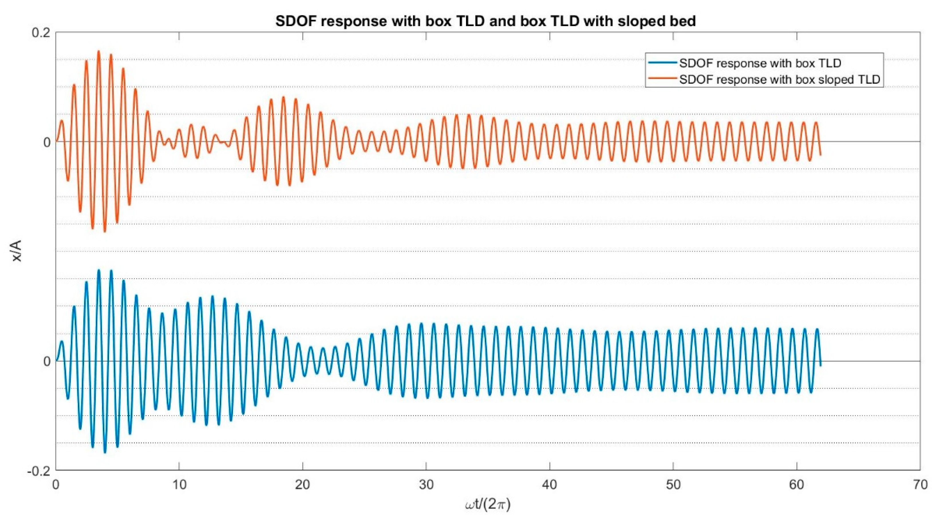
The results of the model for both cases with and without TLDs are shown in Figure 18. Initially, both tanks exhibited minimal influence on the vibration of the structure for a short duration of approximately 1 s after excitation. However, after this initial period, both tanks exhibited significantly reduced structural vibration. Consequently, they are more efficient for far-fault earthquakes than for near faults. Figure 19 presents a close-up view of the SDOF response when equipped with a box TLD or a box sloped-bed TLD. In the steady state, the box sloped-bed TLD exhibited a more profound reduction in structural vibration than the box TLD. In steady state conditions, the amplitude of vibration of the SDOF equipped with a box sloped-bed TLD is approximately 75% of that of the case where the SDOF is equipped with the box TLD. This indicates that the box sloped-bed TLD takes advantage of its smaller water mass and demonstrates a more pronounced suppressing effect on structural vibration in resonance excitation. However, its potentially superior damping effect compared to conventional TLDs in other scenarios requires further investigation.
5. Discussion and Conclusions
This study focuses on developing a numerical model capable of simulating sloshing waves in tanks with both horizontal and sloped beds, which is then coupled with a single-degree-of-freedom (SDOF) system to establish a tuned liquid damper (TLD) model. The model is based on nonlinear shallow water equations and includes additional terms such as the acceleration term, bed slope term, dissipation term, and dispersion term, depending on the specific case study. To balance accuracy and computational cost, the current model employs the central upwind method for approximating flux and the Minmod function for evaluating interface variables. While the slope bed, dissipation, and acceleration terms are treated as explicit source terms in the model, an implicit scheme is utilized for the discretization of the dispersion term to improve model stability, resulting in a matrix equation. Additionally, temporal discretization is achieved using the fourth-order Runge–Kutta method.
The dynamic equation of a single-degree-of-freedom (SDOF) system is numerically solved using a second-order finite difference method. The system of equations, including SDOF dynamics and fluid movement, is coupled with an iterative procedure composed of prediction and correction steps.
The application of the model for simulation of dam break over a dry bed that includes high gradient depth indicates that both the MacCormack scheme, which is a second-order finite difference method, and the Roe scheme produce a nonphysical jump in the free-surface profile, while the central upwind and Roe methods, when equipped with entropy correction, are accurate for modelling this rapid varied flow. Because of the lower computational cost, we adopted the central upwind method for subsequent modelling.
When the current model is applied to a dam break on a sloped bed, it provides accurate results compared to both another numerical model’s outcomes and analytical data. Furthermore, the simulation of perturbed flow over a parabolic bed using the current mode produced a free surface that agreed well with the analytical solutions.
The perturbation of the free-surface test in the box tank indicated that the current model can accurately predict the natural frequency of the tank. In addition, this test was used to measure the numerical diffusion errors of the proposed schemes.
The current model was applied to simulate a box-grounded tank that was subjected to near-resonance excitation. Despite the complexity and asymmetry of the sloshing wave, the present model takes advantage of precise results compared with the experimental data. Neglecting the dispersion term results in nonphysical approximately symmetric shock waves, whereas ignoring the dissipation term prevents the system from reaching steady sloshing waves.
The application of the current model for the sloshing of a box tank with a sloped bed, which requires the contribution of all terms in Equation (1), resulted in more pronounced and stronger sloshing waves compared to the box tank.
In the systematic approach employed in this study, the existing model based on nonlinear shallow water equations was expanded by introducing new terms, the specific selection of which depended on the characteristics of each test case. The accuracy and efficiency of this model were rigorously assessed in the preceding test cases. In the final stage of this research, the model, now encompassing all the pertinent terms, was integrated with a single-degree-of-freedom (SDOF) system to emulate a tuned liquid damper (TLD) featuring a sloped bed. The outcomes derived from this model demonstrate that when the SDOF system undergoes harmonic resonance excitation, a TLD equipped with a sloped bed yields a substantially more pronounced reduction in the SDOF response in comparison with a conventional box TLD. Despite the intricate nature of the simulation, this current model, characterized by its superior accuracy and reasonable computational efficiency, emerges as a suitable tool for TLD modeling even in cases involving sloped beds.
Author Contributions
Conceptualization, M.K. and A.M.; Methodology, M.K. and A.M.; Software, M.K.; Validation, M.K., A.M. and H.S.; Formal analysis, M.K.; Investigation, M.K. and A.M.; Resources, A.M. and H.S.; Data curation, M.K.; Writing—original draft, M.K.; Writing—review & editing, A.M., H.S. and R.K.; Visualization, M.K.; Supervision, A.M., H.S. and R.K.; Project administration, A.M. All authors have read and agreed to the published version of the manuscript.
Funding
This research received no external funding.
Data Availability Statement
Data are contained within the article.
Conflicts of Interest
The authors declare no conflict of interest.
Appendix A. MacCormack Scheme
First, the nonlinear shallow water equations used for the dam break are expressed as follows [38]:
This equation can be converted to the following equation:
The MacCormack scheme, which is a second-order accurate finite difference method, utilizes averaged forward and backward differences for discretization in space [50]. Therefore, the discretized form of Equation (A2) is expressed as follows. Equations (A3) and (A4) correspond to the forward and backward approaches, and Equation (A5) is the averaged variable determined from previous schemes.
References
- Toussi, I.B.; Kianoush, R.; Mohammadian, A. Numerical and Experimental Investigation of Rectangular Liquid-Containing Structures under Seismic Excitation. Infrastructures 2020, 6, 1. [Google Scholar] [CrossRef]
- Liu, D.; Lin, P. A numerical study of three-dimensional liquid sloshing in tanks. J. Comput. Phys. 2008, 227, 3921–3939. [Google Scholar] [CrossRef]
- Vîlceanu, V.; Kavrakov, I.; Morgenthal, G. Coupled numerical simulation of liquid sloshing dampers and wind–structure simulation model. J. Wind. Eng. Ind. Aerodyn. 2023, 240, 105505. [Google Scholar] [CrossRef]
- Hirt, C.W.; Nichols, B.D. Volume of fluid (VOF) method for the dynamics of free boundaries. J. Comput. Phys. 1981, 39, 201–225. [Google Scholar] [CrossRef]
- Veletsos, A.S.; Tang, Y.; Tang, H.T. Dynamic Response of Flexibly Supported Liquid-Storage Tanks. J. Struct. Eng. 1992, 118, 264–283. [Google Scholar] [CrossRef]
- Ghaemmaghami, A.R.; Kianoush, M.R. Effect of Wall Flexibility on Dynamic Response of Concrete Rectangular Liquid Storage Tanks under Horizontal and Vertical Ground Motions. J. Struct. Eng. 2010, 136, 441–451. [Google Scholar] [CrossRef]
- Panigrahy, P.; Saha, U.; Maity, D. Experimental studies on sloshing behavior due to horizontal movement of liquids in baffled tanks. Ocean Eng. 2009, 36, 213–222. [Google Scholar] [CrossRef]
- Virella, J.C.; Suárez, L.E.; Godoy, L.A. A Static Nonlinear Procedure for the Evaluation of the Elastic Buckling of Anchored Steel Tanks Due to Earthquakes. J. Earthq. Eng. 2008, 12, 999–1022. [Google Scholar] [CrossRef]
- Sobhan, M.; Rofooei, F.; Attari, N.K. Buckling behavior of the anchored steel tanks under horizontal and vertical ground motions using static pushover and incremental dynamic analyses. Thin-Walled Struct. 2017, 112, 173–183. [Google Scholar] [CrossRef]
- Hashemi, S.; Kianoush, R.; Khoubani, M. A mechanical model for soil-rectangular tank interaction effects under seismic loading. Soil Dyn. Earthq. Eng. 2021, 153, 107092. [Google Scholar] [CrossRef]
- Sriram, V.; Sannasiraj, S.A.; Sundar, V. Numerical simulation of 2D sloshing waves due to horizontal and vertical random excitation. Applied Ocean Research 2006, 28, 19–32. [Google Scholar] [CrossRef]
- Ikeda, T.; Ibrahim, R.A.; Harata, Y.; Kuriyama, T. Nonlinear liquid sloshing in a square tank subjected to obliquely horizontal excitation. J. Fluid Mech. 2012, 700, 304–328. [Google Scholar] [CrossRef]
- Antuono, M.; Bouscasse, B.; Colagrossi, A.; Lugni, C. Two-dimensional modal method for shallow-water sloshing in rectangular basins. J. Fluid Mech. 2012, 700, 419–440. [Google Scholar] [CrossRef]
- Saburin, D.S. Tank sloshing simulations in shallow-water approximation. In MARINE VI: Proceedings of the VI International Conference on Computational Methods in Marine Engineering; CIMNE: Barcelona, Spain, 2015; pp. 1039–1050. [Google Scholar]
- Sun, L.M.; Fujino, Y.; Pacheco, B.M.; Chaiseri, P. Modelling of tuned liquid damper (TLD). J. Wind. Eng. Ind. Aerodyn. 1992, 43, 1883–1894. [Google Scholar] [CrossRef]
- Koh, C.G.; Mahatma, S.; Wang, C.M. Theoretical and experimental studies on rectangular liquid dampers under arbitrary excitations. Earthq. Eng. Struct. Dyn. 1994, 23, 17–31. [Google Scholar] [CrossRef]
- Tait, M.; El Damatty, A.; Isyumov, N.; Siddique, M. Numerical flow models to simulate tuned liquid dampers (TLD) with slat screens. J. Fluids Struct. 2005, 20, 1007–1023. [Google Scholar] [CrossRef]
- Murudi, M.; Banerji, P. Effective control of earthquake response using tuned liquid dampers. J. Earthq. Technol. 2012, 49, 53–71. [Google Scholar]
- Banerji, P.; Samanta, A.; Chavan, S.A. Earthquake vibration control of structures using tuned liquid dampers: Experimental studies. Int. J. Adv. Struct. Eng. 2010, 2, 133–152. [Google Scholar]
- Konar, T.; Ghosh, A.D. Flow Damping Devices in Tuned Liquid Damper for Structural Vibration Control: A Review. Arch. Comput. Methods Eng. 2020, 28, 2195–2207. [Google Scholar] [CrossRef]
- Abd-Elhamed, A.; Tolan, M. Tuned liquid damper for vibration mitigation of seismic-excited structures on soft soil. Alex. Eng. J. 2022, 61, 9583–9599. [Google Scholar] [CrossRef]
- Pandit, A.R.; Biswal, K.C. Seismic Control of Structures Using Sloped Bottom Tuned Liquid Damper. Int. J. Struct. Stab. Dyn. 2019, 19, 1950096. [Google Scholar] [CrossRef]
- Chaiviriyawong, P.; Webster, W.; Pinkaew, T.; Lukkunaprasit, P. Simulation of characteristics of tuned liquid column damper using a potential-flow method. Eng. Struct. 2007, 29, 132–144. [Google Scholar] [CrossRef]
- Banerji, P.; Murudi, M.; Shah, A.H.; Popplewell, N. Tuned liquid dampers for controlling earthquake response of structures. Earthq. Eng. Struct. Dyn. 2000, 29, 587–602. [Google Scholar] [CrossRef]
- Fujino, Y.; Sun, L.; Pacheco, B.M.; Chaiseri, P. Tuned Liquid Damper (TLD) for Suppressing Horizontal Motion of Structures. J. Eng. Mech. 1992, 118, 2017–2030. [Google Scholar] [CrossRef]
- Marivani, M.; Hamed, M. Evaluate pressure drop of slat screen in an oscillating fluid in a tuned liquid damper. Comput. Fluids 2017, 156, 384–401. [Google Scholar] [CrossRef]
- Zhao, Z.; Zhang, R.; Jiang, Y.; Pan, C. A tuned liquid inerter system for vibration control. Int. J. Mech. Sci. 2019, 164, 105171. [Google Scholar] [CrossRef]
- Wang, Q.; Tiwari, N.D.; Qiao, H.; Wang, Q. Inerter-based tuned liquid column damper for seismic vibration control of a single-degree-of-freedom structure. Int. J. Mech. Sci. 2020, 184, 105840. [Google Scholar] [CrossRef]
- Ashasi-Sorkhabi, A.; Malekghasemi, H.; Ghaemmaghami, A.; Mercan, O. Experimental investigations of tuned liquid damper-structure interactions in resonance considering multiple parameters. J. Sound Vib. 2017, 388, 141–153. [Google Scholar] [CrossRef]
- Saha, S.; Debbarma, R. An experimental study on response control of structures using multiple tuned liquid dampers under dynamic loading. Int. J. Adv. Struct. Eng. 2016, 9, 27–35. [Google Scholar] [CrossRef]
- Hu, X.; Zhao, Z.; Weng, D.; Hu, D. Design of a pair of isolated tuned liquid dampers (ITLDs) and application in multi-degree-of-freedom structures. Int. J. Mech. Sci. 2022, 217, 107027. [Google Scholar] [CrossRef]
- Bhattacharjee, E.; Halder, L.; Sharma, R.P. An experimental study on tuned liquid damper for mitigation of structural response. Int. J. Adv. Struct. Eng. 2013, 5, 3. [Google Scholar] [CrossRef]
- Samanta, A.; Banerji, P. Structural vibration control using modified tuned liquid dampers. IES J. Part A Civ. Struct. Eng. 2010, 3, 14–27. [Google Scholar] [CrossRef]
- Chang, Y.; Noormohamed, A.; Mercan, O. Analytical and experimental investigations of Modified Tuned Liquid Dampers (MTLDs). J. Sound Vib. 2018, 428, 179–194. [Google Scholar] [CrossRef]
- Ocak, A.; Bekdaş, G.; Nigdeli, S.M.; Kim, S.; Geem, Z.W. Optimization of Tuned Liquid Damper Including Different Liquids for Lateral Displacement Control of Single and Multi-Story Structures. Buildings 2022, 12, 377. [Google Scholar] [CrossRef]
- Pandit, A.; Biswal, K. Seismic control of multi degree of freedom structure outfitted with sloped bottom tuned liquid damper. Structures 2020, 25, 229–240. [Google Scholar] [CrossRef]
- Gardarsson, S.; Yeh, H.; Reed, D. Behavior of Sloped-Bottom Tuned Liquid Dampers. J. Eng. Mech. 2001, 127, 266–271. [Google Scholar] [CrossRef]
- Toro, E.F. Shock-Capturing Methods for Free-Surface Shallow Flows; Wiley and Sons Ltd.: Hoboken, NJ, USA, 2001; pp. 1–309. [Google Scholar]
- Benkhaldoun, F.; Seaïd, M. A simple finite volume method for the shallow water equations. J. Comput. Appl. Math. 2010, 234, 58–72. [Google Scholar] [CrossRef]
- Ardakani, H.A.; Bridges, T. Shallow-water sloshing in vessels undergoing prescribed rigid-body motion in two dimensions. Eur. J. Mech.-B/Fluids 2012, 31, 30–43. [Google Scholar] [CrossRef]
- Mohammadian, A.; Le Roux, D.Y. Simulation of shallow flows over variable topographies using unstructured grids. Int. J. Numer. Methods Fluids 2006, 52, 473–498. [Google Scholar] [CrossRef]
- Kurganov, A.; Levy, D. Central-upwind schemes for the Saint-Venant system. ESAIM Math. Model. Numer. Anal. 2002, 36, 397–425. [Google Scholar] [CrossRef]
- Mohammadian, A.; Le Roux, D.; Tajrishi, M. A conservative extension of the method of characteristics for 1-D shallow flows. Appl. Math. Model. 2007, 31, 332–348. [Google Scholar] [CrossRef]
- Durran, D.R. Numerical Methods for Fluid Dynamics: With Applications to Geophysics; Springer Science & Business Media: Berlin/Heidelberg, Germany, 2010; Volume 32. [Google Scholar]
- Humar, J. Dynamics of Structures; CRC Press: Boca Raton, FL, USA, 2012. [Google Scholar]
- Chopra, A.K. Dynamics of Structures; Pearson Education India: Chennai, India, 2007. [Google Scholar]
- Liao, K.; Hu, C. A coupled FDM–FEM method for free surface flow interaction with thin elastic plate. J. Mar. Sci. Technol. 2012, 18, 1–11. [Google Scholar] [CrossRef]
- MacCormack, R.W. Numerical solution of the interaction of a shock wave with a laminar boundary layer. In Proceedings of the Second International Conference on Numerical Methods in Fluid Dynamics, University of California, Berkeley, CA, USA, 15–19 September 1970; Springer: Berlin/Heidelberg, Germany, 2005; pp. 151–163. [Google Scholar]
- Chaudhry, M.H.; Hussaini, M.Y. Second-order accurate explicit finite-difference schemes for waterhammer analysis. J. Fluids Eng. 1985, 107, 523–529. [Google Scholar] [CrossRef]
- Amara, L.; Berreksi, A.; Achour, B. Adapted MacCormack Finite-Differences Scheme for Water Hammer Simulation. J. Civ. Eng. Sci. 2013, 2, 226–233. [Google Scholar]
- Fennema, R.J.; Chaudhry, M.H. Explicit numerical schemes for unsteady free-surface flows with shocks. Water Resour. Res. 1986, 22, 1923–1930. [Google Scholar] [CrossRef]
- Garcia, R.; Kahawita, R.A. Numerical solution of the St. Venant equations with the MacCormack finite-difference scheme. Int. J. Numer. Methods Fluids 1986, 6, 259–274. [Google Scholar] [CrossRef]
- van Leer, B.; Lee, W.T.; Powell, K.G. Sonic point capturing. In Proceedings of the 9th CFD Conference, Buffalo, NY, USA, 13–15 June 1989. [Google Scholar]
- Bradford, S.F.; Sandres, B.F. Finite-volume model for shallow-water fooding of arbitrary topography. J. Hydraul. Eng. (ASCE) 2002, 128, 289–298. [Google Scholar] [CrossRef]
- Xing, Y.; Zhang, X.; Shu, C.-W. Positivity-preserving high order well-balanced discontinuous Galerkin methods for the shallow water equations. Adv. Water Resour. 2010, 33, 1476–1493. [Google Scholar] [CrossRef]
- Zhu, Z.; Yang, Z.; Bai, F.; An, R. A New Well-Balanced Reconstruction Technique for the Numerical Simulation of Shallow Water Flows with Wet/Dry Fronts and Complex Topography. Water 2018, 10, 1661. [Google Scholar] [CrossRef]
- Sampson, J.; Easton, A.; Singh, M. Moving boundary shallow water flow above parabolic bottom topography. Anziam J. 2006, 47, 373–387. [Google Scholar] [CrossRef]
- Lepelletier, T.G.; Raichlen, F. Nonlinear Oscillations in Rectangular Tanks. J. Eng. Mech. 1988, 114, 1–23. [Google Scholar] [CrossRef]
- Wu, G.; Ma, Q.; Taylor, R.E. Numerical simulation of sloshing waves in a 3D tank based on a finite element method. Appl. Ocean Res. 1998, 20, 337–355. [Google Scholar] [CrossRef]
- Cao, X.; Ming, F.; Zhang, A. Sloshing in a rectangular tank based on SPH simulation. Appl. Ocean Res. 2014, 47, 241–254. [Google Scholar] [CrossRef]
Figure 1.
Schematic of shallow water equation parameters.

Figure 2.
Schematic of control volume and control surfaces of node j.
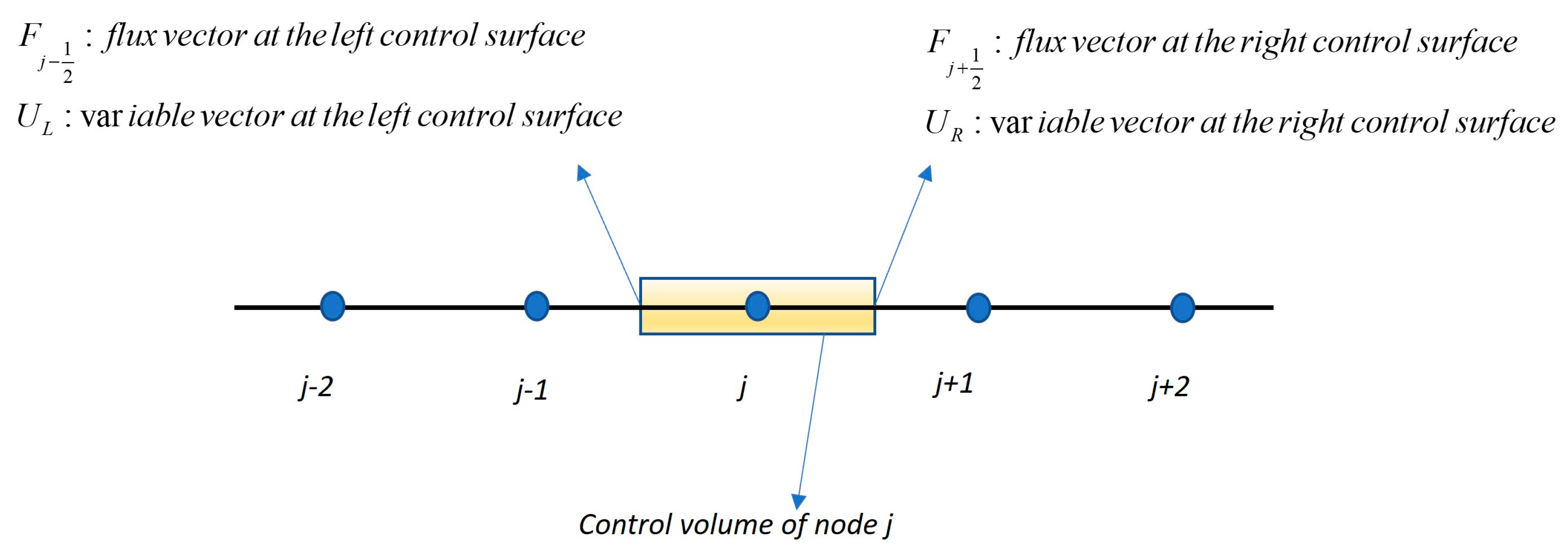
Figure 3.
Schematic of SDOF subjected to ground excitation from the bottom and water tank sloshing from the top.
Figure 3.
Schematic of SDOF subjected to ground excitation from the bottom and water tank sloshing from the top.
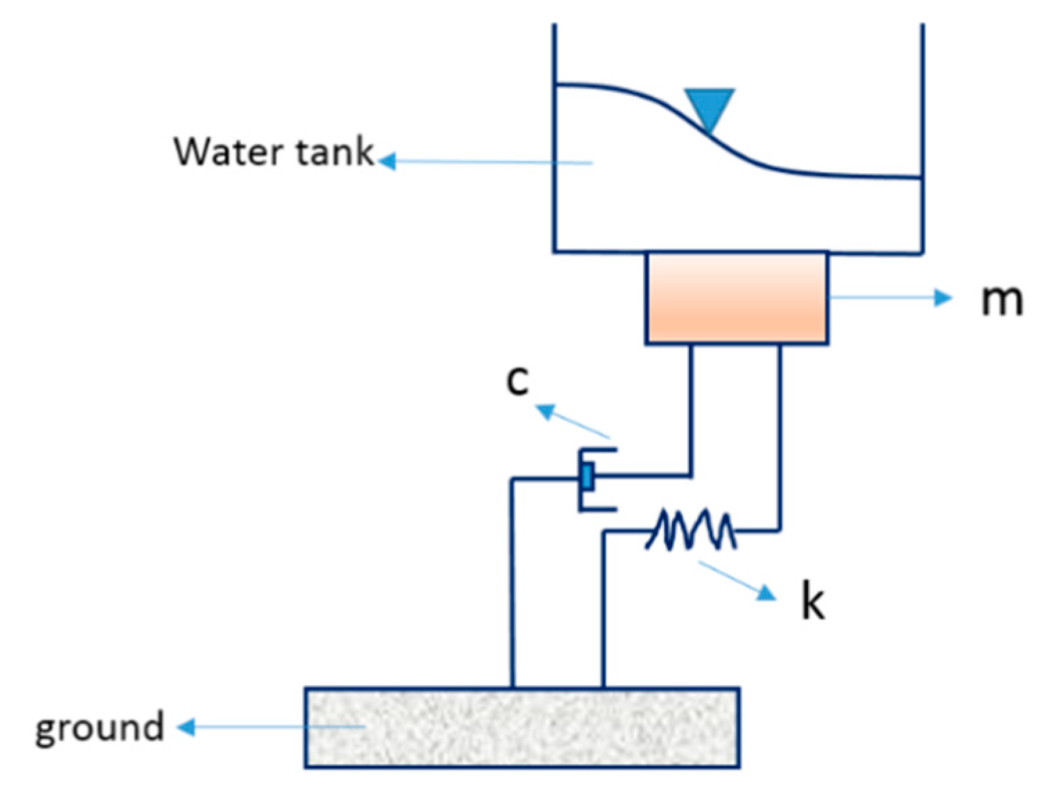
Figure 4.
Flowchart of the coupling system for TLD simulation.

Figure 5.
Comparison of analytical solution of dam break on the horizontal dry bed with those obtained using (a) central upwind method and MacCormack method and (b) Roe scheme with and without entropy correction.
Figure 5.
Comparison of analytical solution of dam break on the horizontal dry bed with those obtained using (a) central upwind method and MacCormack method and (b) Roe scheme with and without entropy correction.
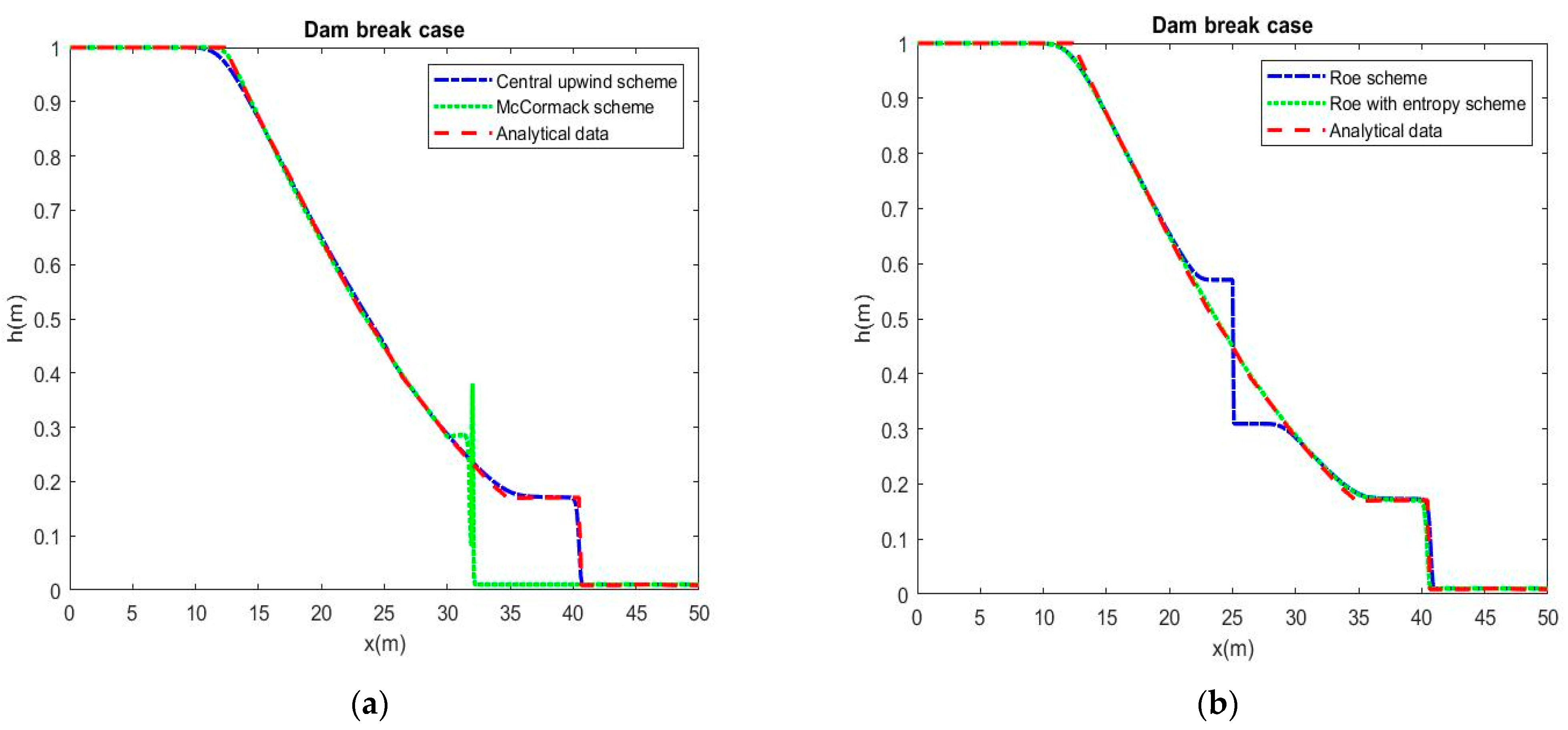
Figure 6.
Free surface obtained from the present numerical model and the model of Zhu et al. [56] for a dam break over a sloped bed ().
Figure 6.
Free surface obtained from the present numerical model and the model of Zhu et al. [56] for a dam break over a sloped bed ().
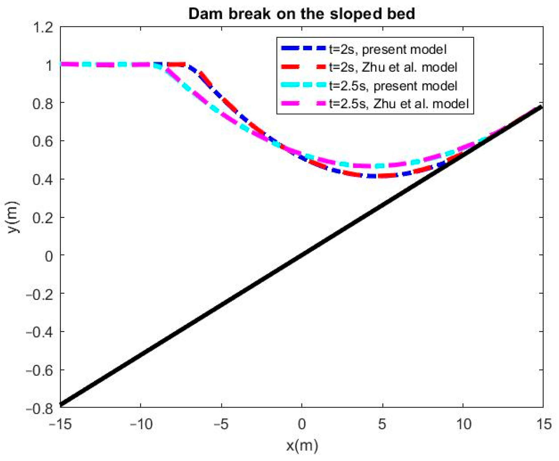
Figure 7.
Wet/dry front position obtained from present numerical model and the model of Zhu et al. [56], as well as an analytical solution for (a) and (b) .
Figure 7.
Wet/dry front position obtained from present numerical model and the model of Zhu et al. [56], as well as an analytical solution for (a) and (b) .
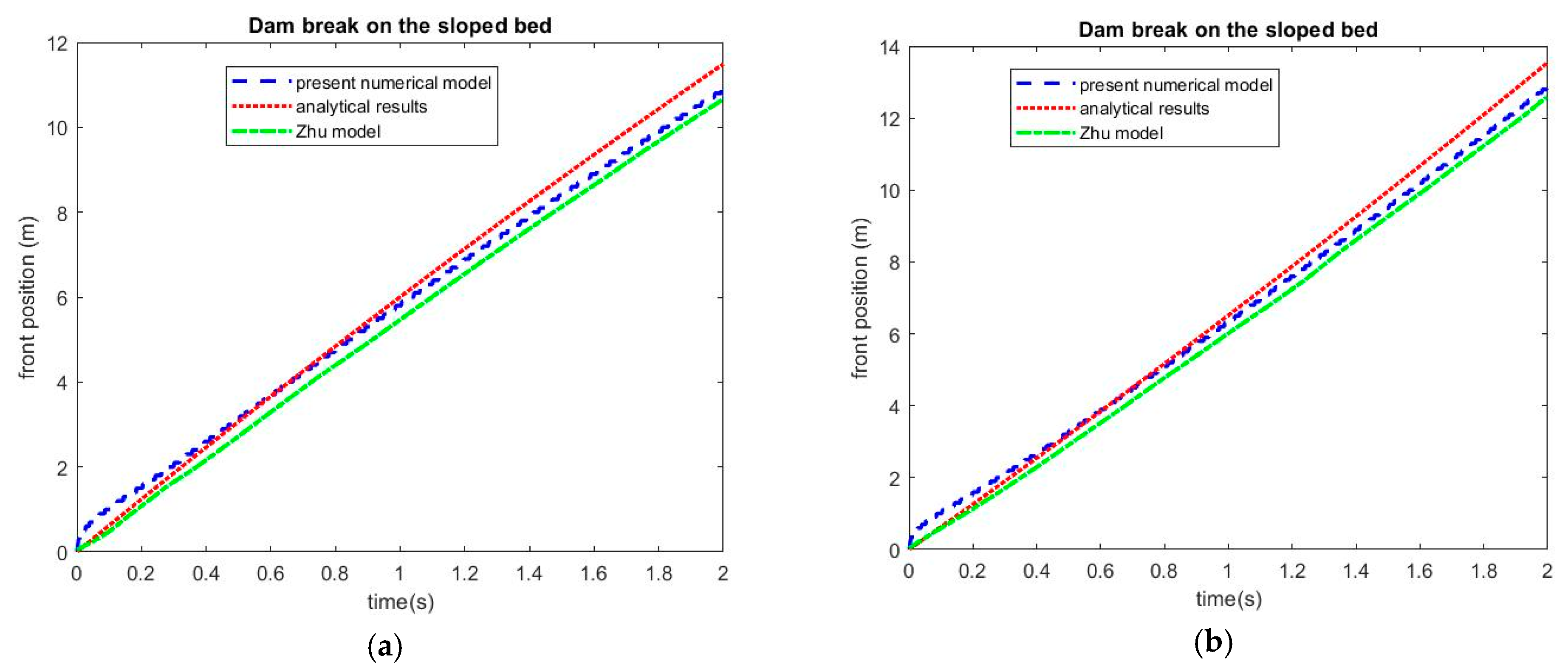
Figure 8.
Comparison of the present numerical model’s results with analytical expression for different times: (a) t = 1000 s, (b) t = 2000 s, (c) t = 4000 s, and (d) t = 6000 s.
Figure 8.
Comparison of the present numerical model’s results with analytical expression for different times: (a) t = 1000 s, (b) t = 2000 s, (c) t = 4000 s, and (d) t = 6000 s.
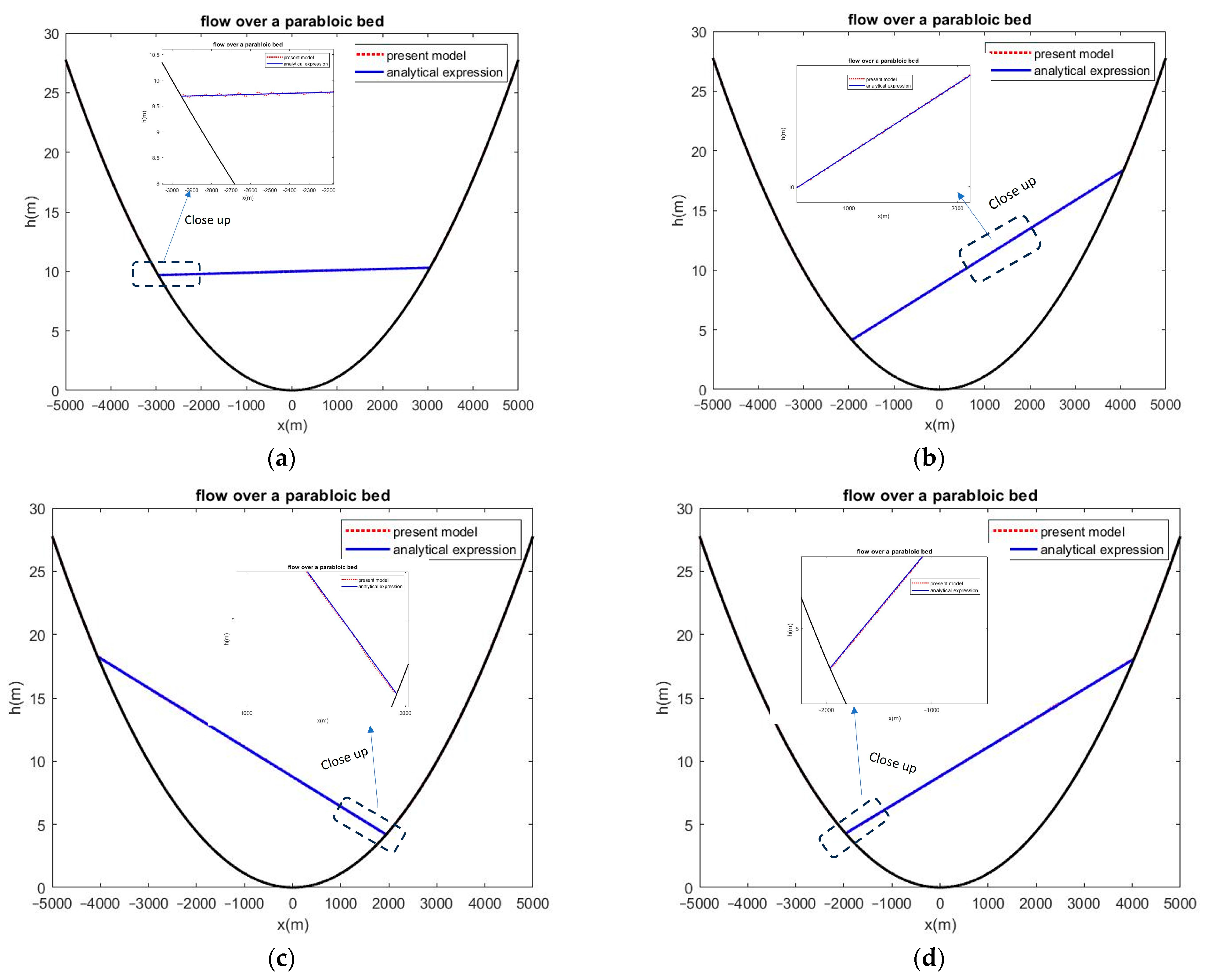
Figure 9.
Time history of the free surface at the right wall of the tank subjected to initial perturbation.
Figure 9.
Time history of the free surface at the right wall of the tank subjected to initial perturbation.
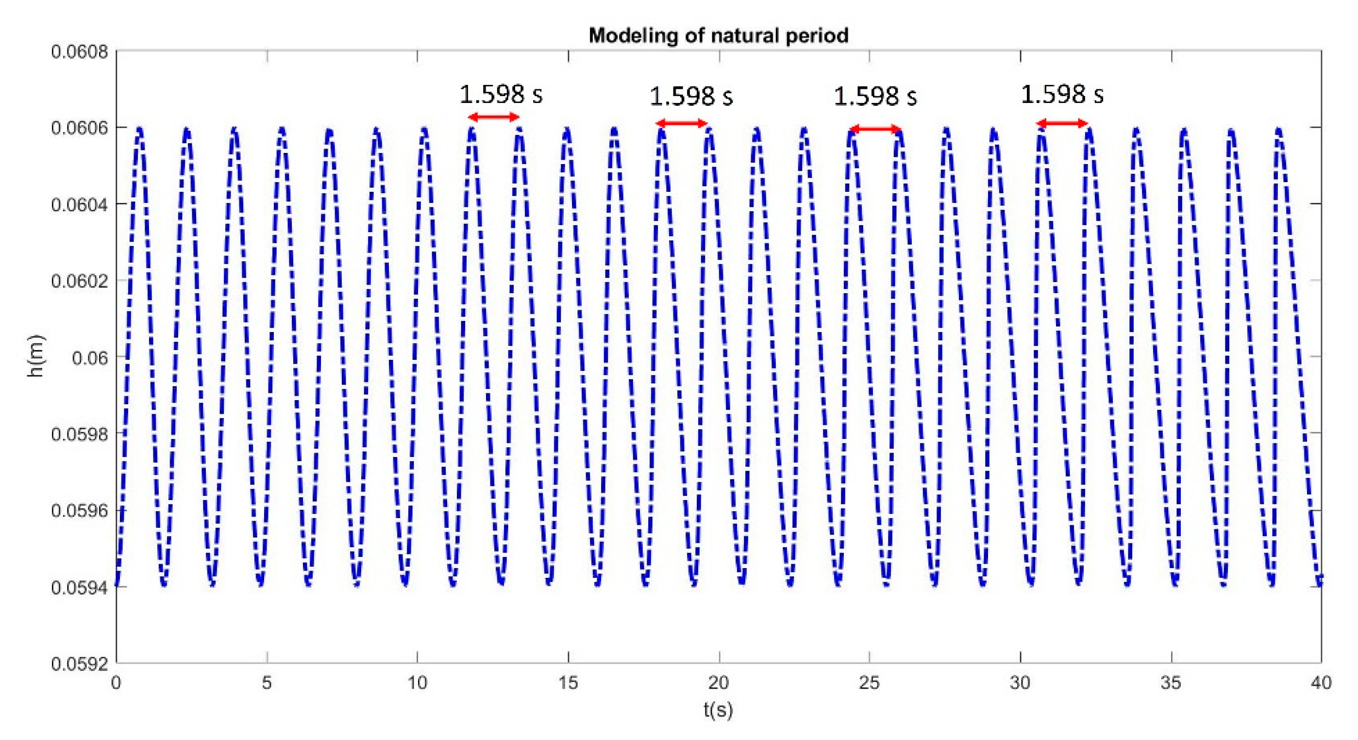
Figure 10.
Numerical diffusion errors in perturbation tests associated with first-order upwind and Minmod schemes.
Figure 10.
Numerical diffusion errors in perturbation tests associated with first-order upwind and Minmod schemes.
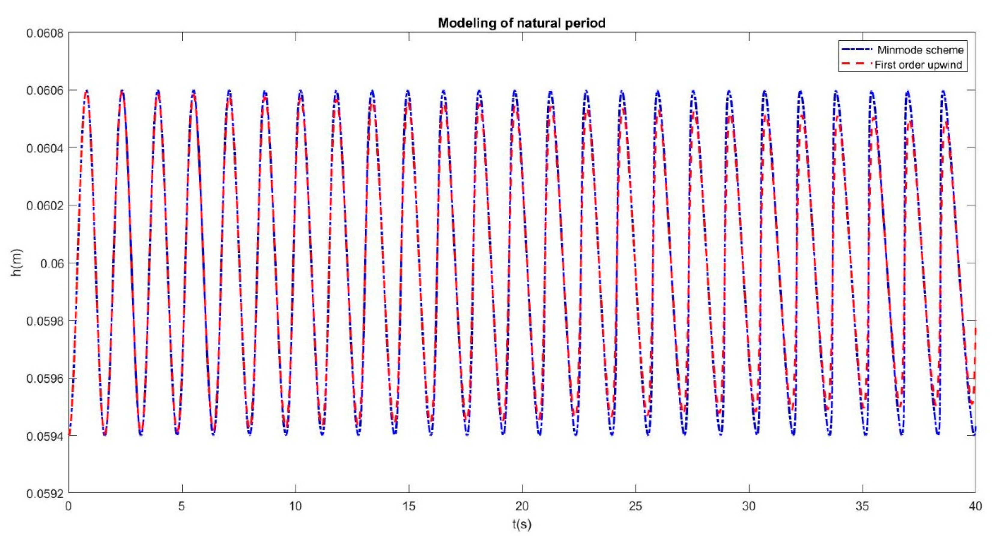
Figure 11.
Time history of wave height at the right wall of the tank subjected to near-resonance excitations derived from (a) the experimental results of Lepelletier et al. [58] and (b) the present numerical model.
Figure 11.
Time history of wave height at the right wall of the tank subjected to near-resonance excitations derived from (a) the experimental results of Lepelletier et al. [58] and (b) the present numerical model.
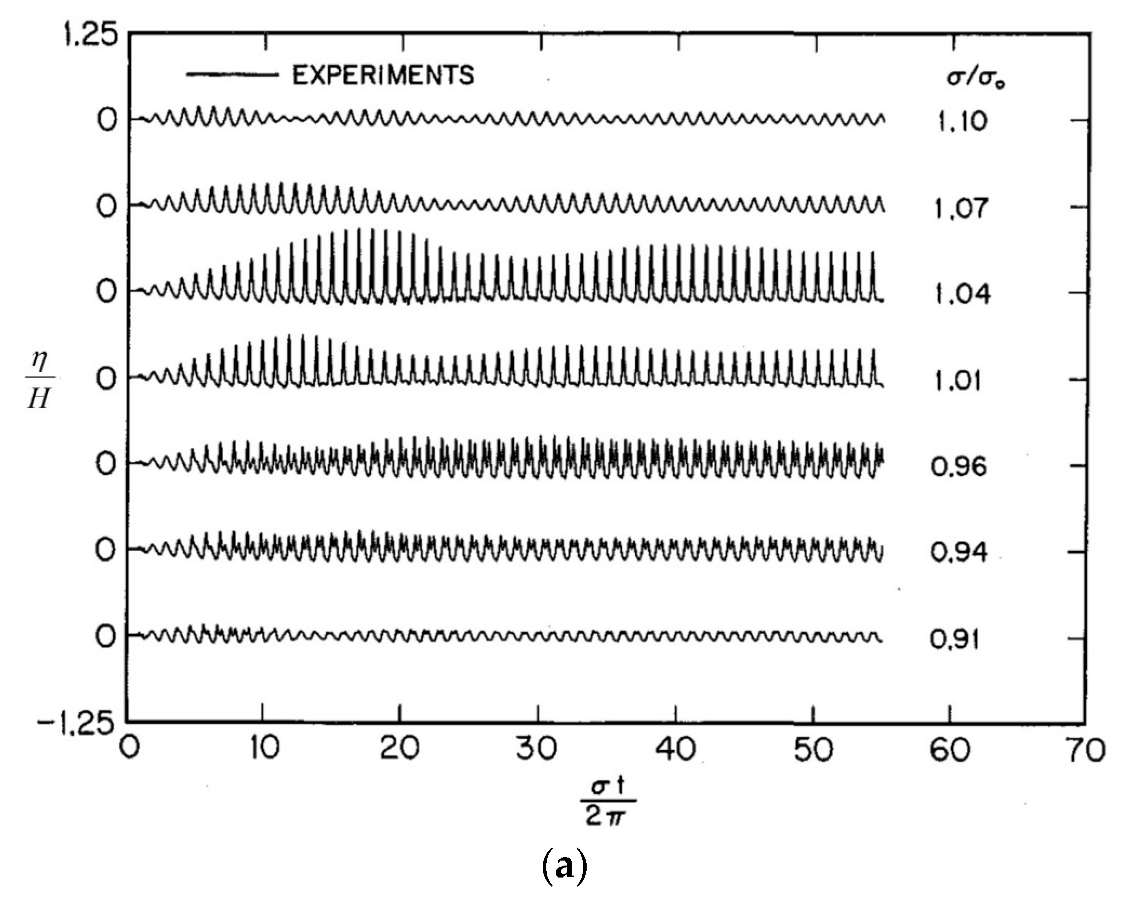
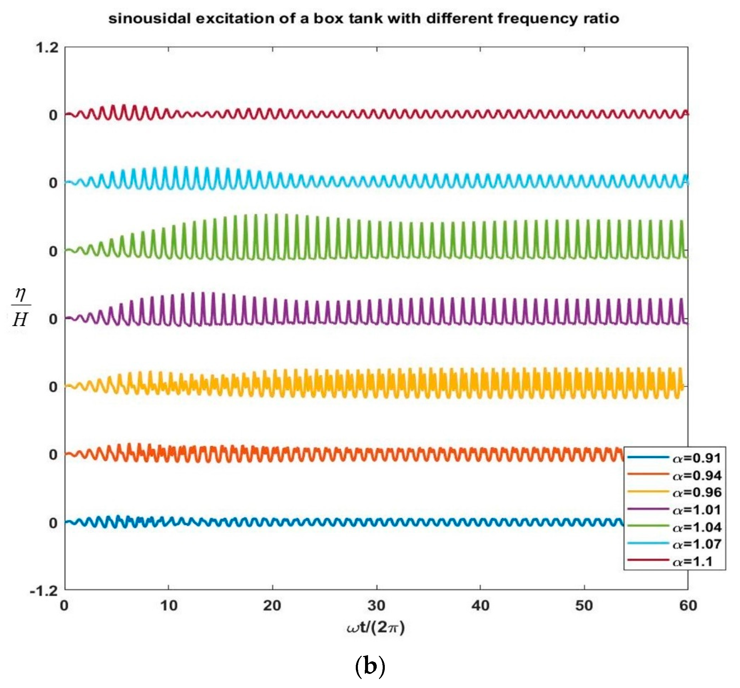
Figure 12.
Time history of wave height with and without the dispersion term.
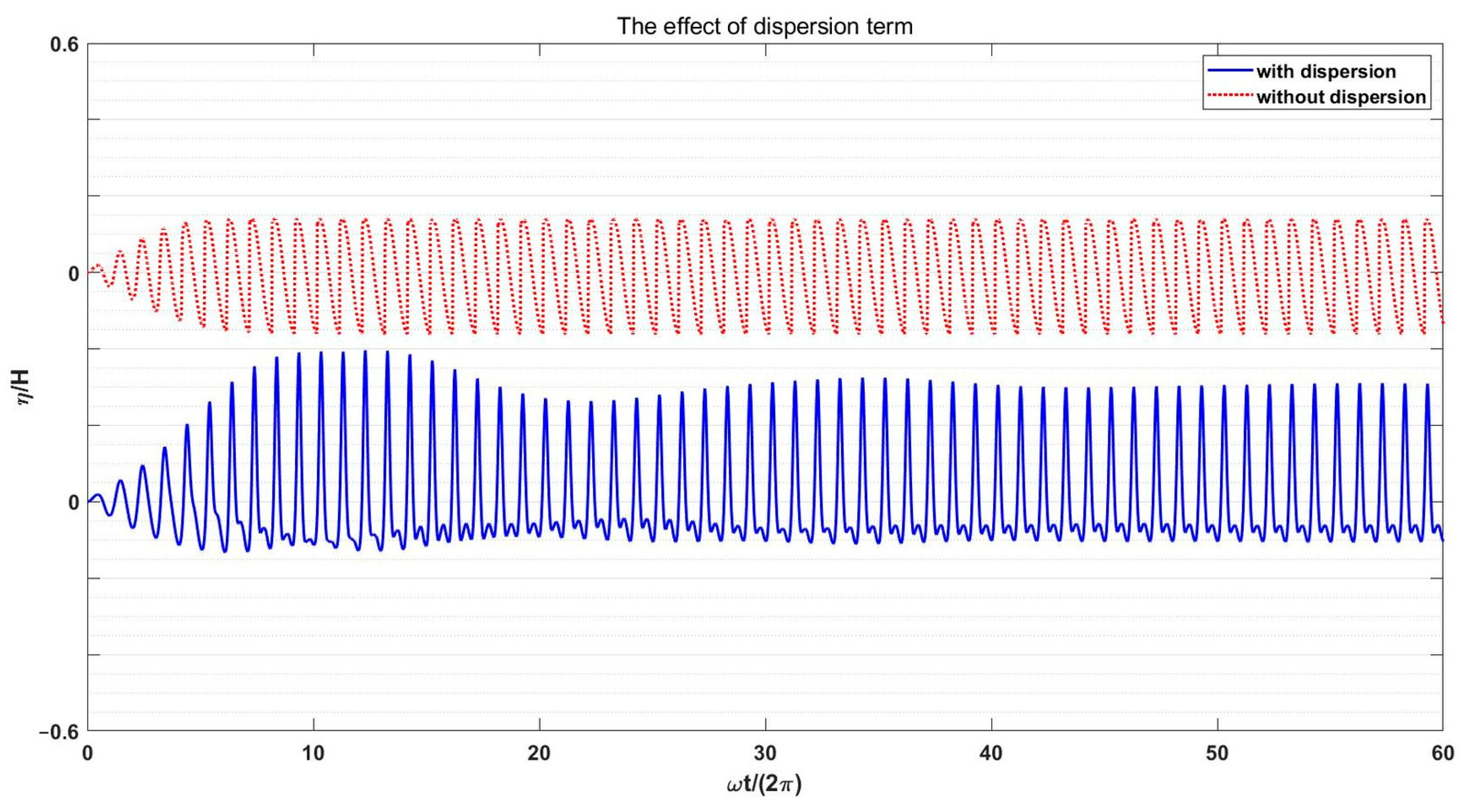
Figure 13.
Transient and steady waves formed in a sloshing experimental test (based [58]).
Figure 13.
Transient and steady waves formed in a sloshing experimental test (based [58]).

Figure 14.
Time history of wave height with and without the dissipation term.
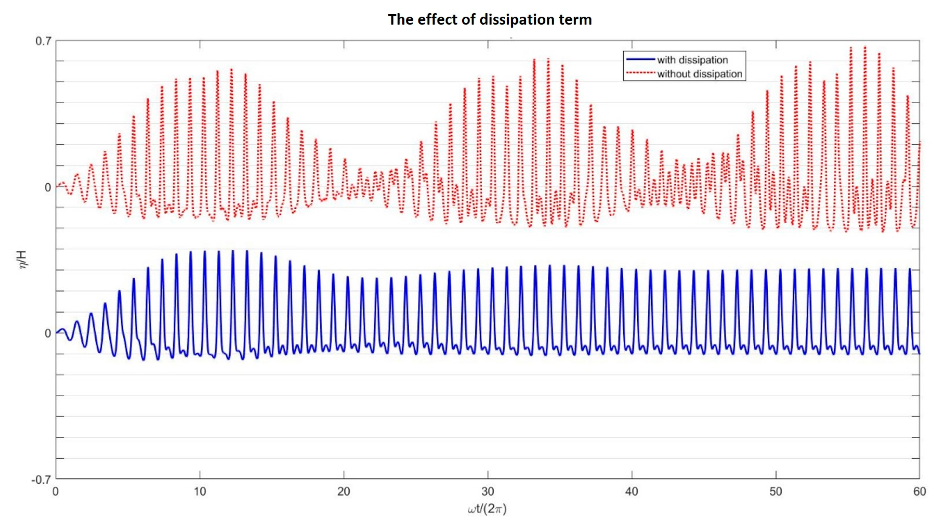
Figure 15.
Geometry of the box tank with a sloped bed.

Figure 16.
Time history of wave height at the right wall of the box tank (bottom) and the box tank with a sloped bed (top) subjected to resonance excitation.
Figure 16.
Time history of wave height at the right wall of the box tank (bottom) and the box tank with a sloped bed (top) subjected to resonance excitation.
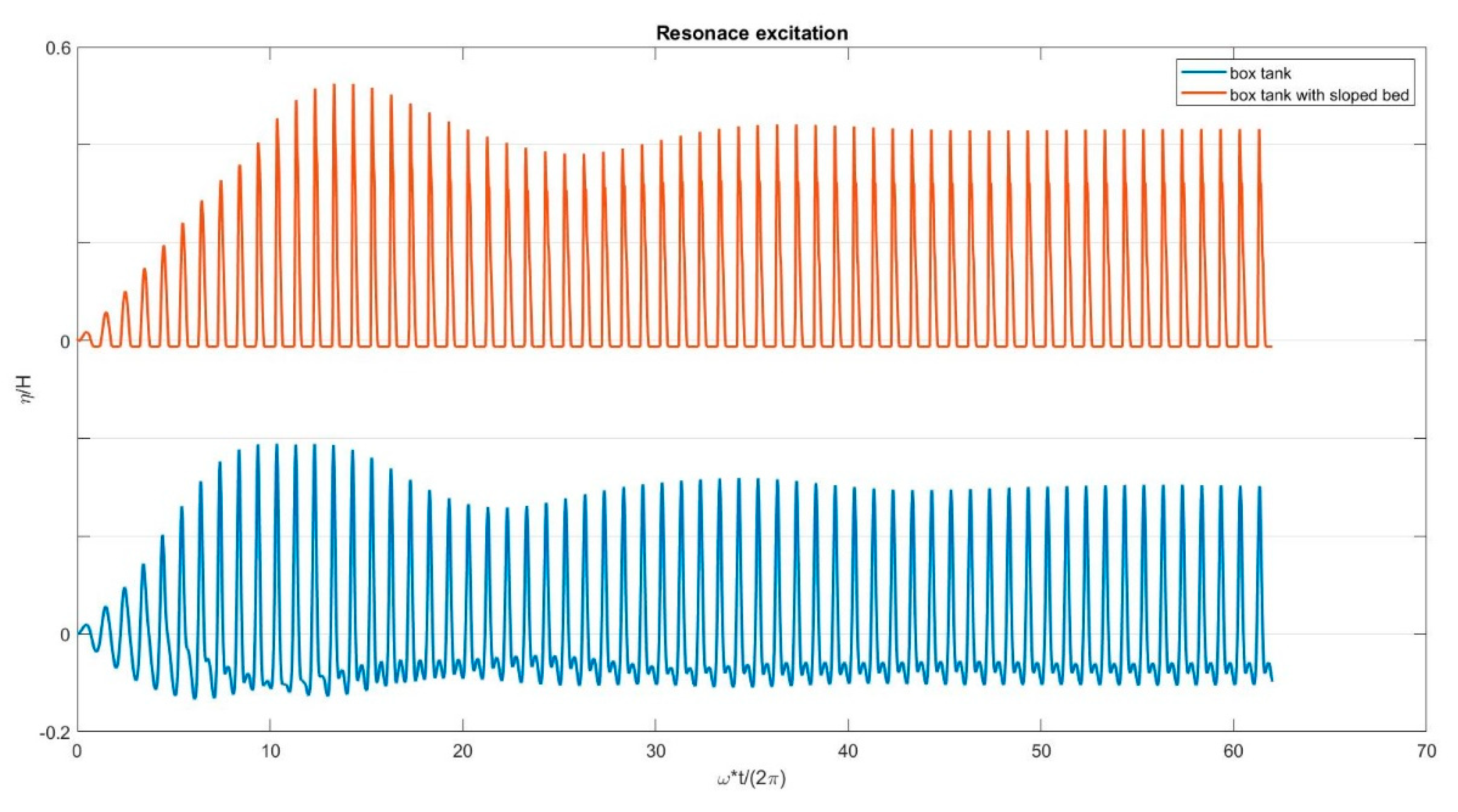
Figure 17.
Different scenarios for the evaluation of the pressure force acting on the right wall. (a): Rectangular box, (b): Sloped bed TLD with free surface at the right vertical wall, (c): Sloped bed TLD with free surface at the right sloped bed.
Figure 17.
Different scenarios for the evaluation of the pressure force acting on the right wall. (a): Rectangular box, (b): Sloped bed TLD with free surface at the right vertical wall, (c): Sloped bed TLD with free surface at the right sloped bed.
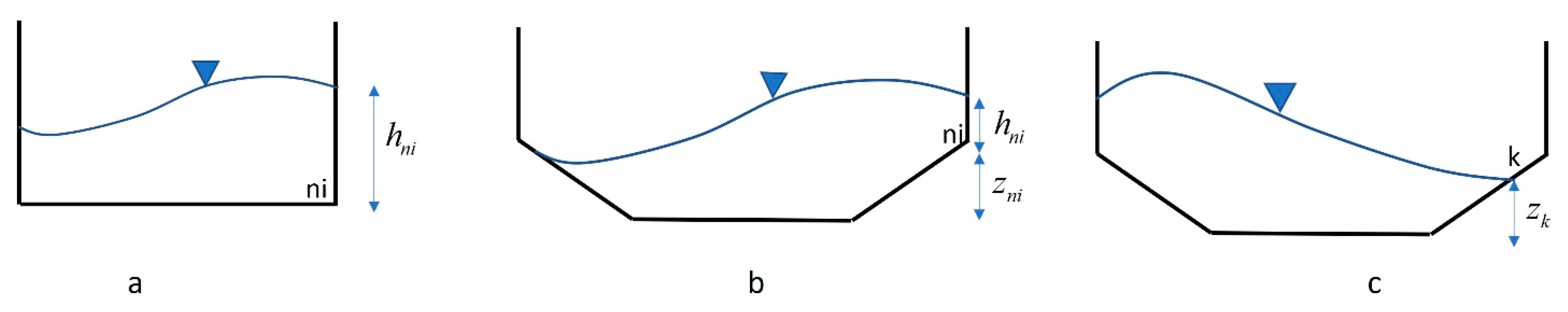
Figure 18.
The response of SOF equipped with and without TLD for two cases: box TLD (bottom) and box TLD with a sloped bed (top).
Figure 18.
The response of SOF equipped with and without TLD for two cases: box TLD (bottom) and box TLD with a sloped bed (top).
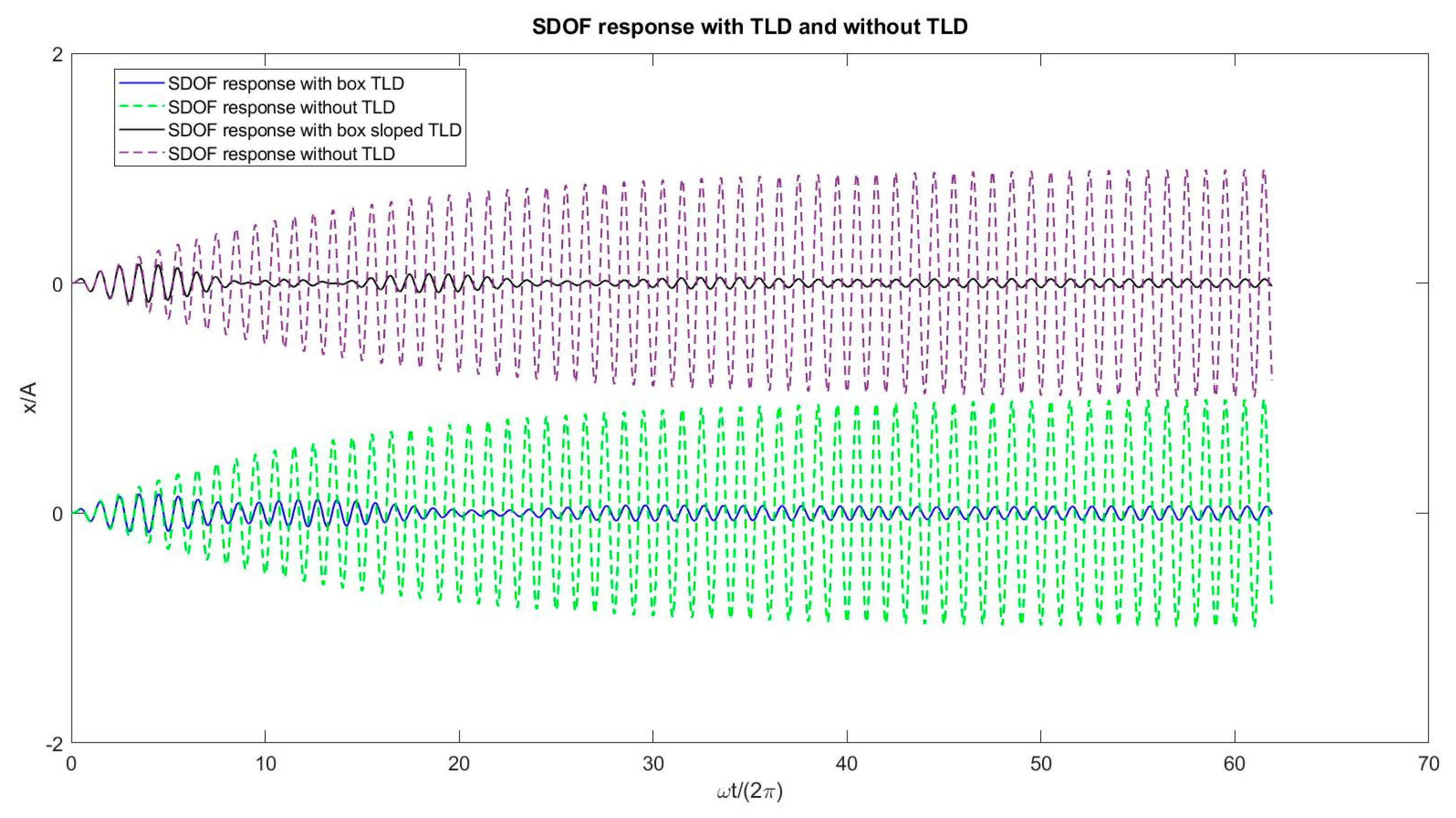
Figure 19.
Close-up view of the SDOF response when it is equipped with TLD for two cases: box TLD (bottom) and box TLD with a sloped bed (top).
Figure 19.
Close-up view of the SDOF response when it is equipped with TLD for two cases: box TLD (bottom) and box TLD with a sloped bed (top).
Disclaimer/Publisher’s Note: The statements, opinions and data contained in all publications are solely those of the individual author(s) and contributor(s) and not of MDPI and/or the editor(s). MDPI and/or the editor(s) disclaim responsibility for any injury to people or property resulting from any ideas, methods, instructions or products referred to in the content. |
© 2024 by the authors. Licensee MDPI, Basel, Switzerland. This article is an open access article distributed under the terms and conditions of the Creative Commons Attribution (CC BY) license (https://creativecommons.org/licenses/by/4.0/).
Share and Cite
MDPI and ACS Style
Khanpour, M.; Mohammadian, A.; Shirkhani, H.; Kianoush, R. Simulation of Sloped-Bed Tuned Liquid Dampers Using a Nonlinear Shallow Water Model. Water 2024, 16, 1394. https://doi.org/10.3390/w16101394
AMA Style
Khanpour M, Mohammadian A, Shirkhani H, Kianoush R. Simulation of Sloped-Bed Tuned Liquid Dampers Using a Nonlinear Shallow Water Model. Water. 2024; 16(10):1394. https://doi.org/10.3390/w16101394
Chicago/Turabian StyleKhanpour, Mahdiyar, Abdolmajid Mohammadian, Hamidreza Shirkhani, and Reza Kianoush. 2024. "Simulation of Sloped-Bed Tuned Liquid Dampers Using a Nonlinear Shallow Water Model" Water 16, no. 10: 1394. https://doi.org/10.3390/w16101394
Note that from the first issue of 2016, this journal uses article numbers instead of page numbers. See further details here.