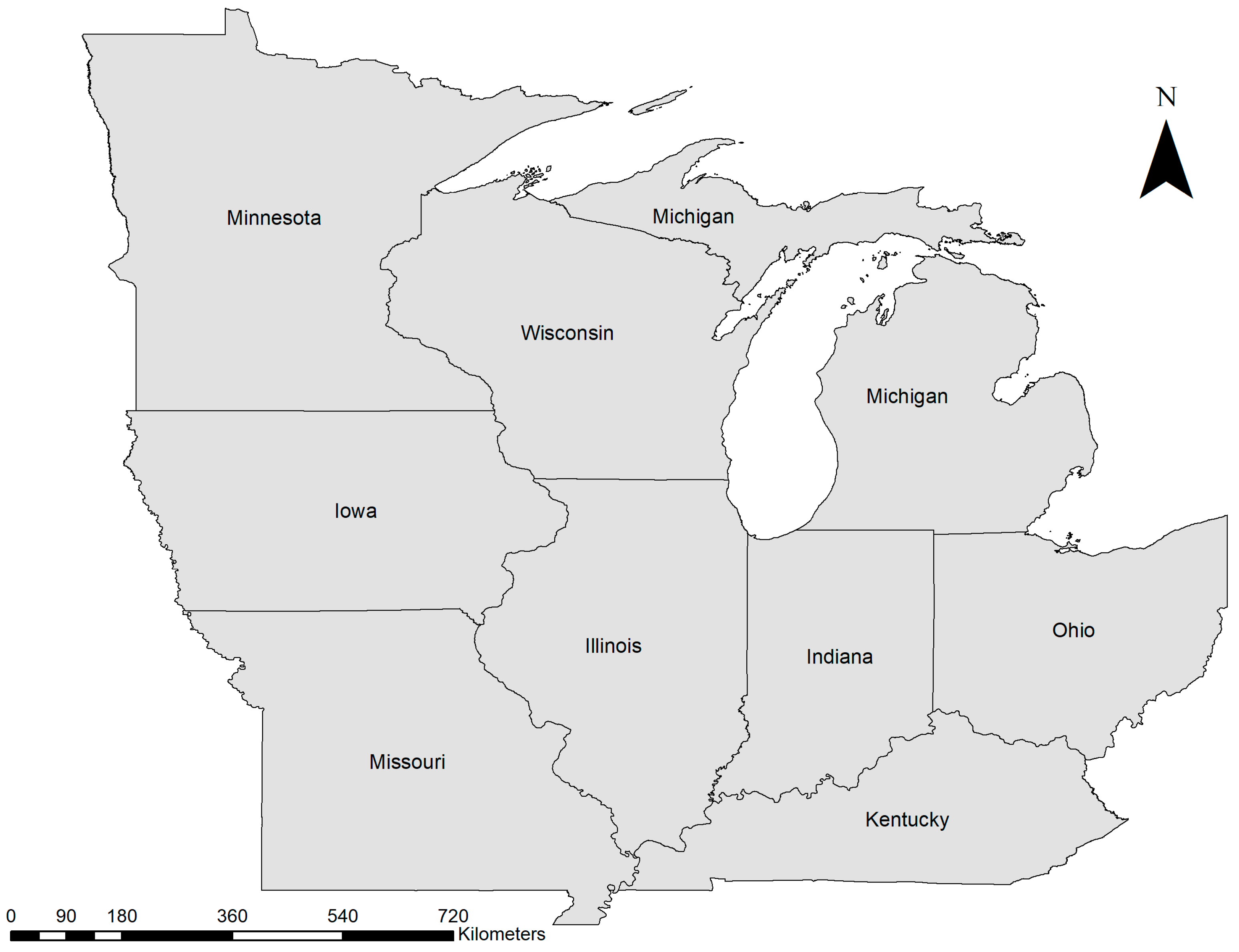
Assessment of Deadly Heat Stress and Extreme Cold Events in the Upper Midwestern United States

Abstract

Understanding and addressing the implications of extreme temperature-related events are critical under climate change, as they directly impact public health and strain energy infrastructure. This study delved into the critical assessment of deadly heat stress and extreme cold events in the Upper Midwestern United States (UMUS), from 1979 to 2021, recognizing the substantial and disparate impact these phenomena have on socially vulnerable communities. In the current study, the modified Mann–Kendall method was applied to understand the temporal trend of extreme heat stress, as well as extreme cold events, from 1979 to 2021 in the UMUS. The results showed that the average annual frequency of daytime extreme heat stress events was comparatively lower in the northern parts of the UMUS compared to the southern parts from 1979 to 2021. Furthermore, a significant increasing trend in daytime extreme heat stress was found in parts of Michigan, Wisconsin (around the lake region), Ohio, and lower parts of Indiana and Kentucky from 1979 to 2021. In contrast, a decreasing trend was noticed in western parts of the UMUS (parts of Minnesota, Iowa, and Missouri). A significant decreasing trend in extreme cold events was found throughout the UMUS from 1979 to 2021. However, an increasing trend was also noticed in Iowa and northern parts of Minnesota, Michigan, and Wisconsin. The results provide important insights for better understanding the unique risks posed by extreme temperature-related events, especially toward socially vulnerable communities in the UMUS, which is crucial for developing targeted interventions and fostering resilience in the face of escalating climate-related threats.

1. Introduction

The current global warming will probably exacerbate the characteristics of extreme events, including extreme heat in terms of its frequency and severity [1,2,3,4,5]. A significant amount of research indicates that heat waves and extreme hot weather conditions are associated with an increase in both mortality rates and morbidity [6,7]. According to a study by [8], a significant portion of the world’s population (around 30%) experiences deadly heat for at least 20 days annually. This number was projected to rise to 48–74% by 2100 due to global warming. The study by [9] indicated that, as the temperature continues to increase, there will be a growing number of individuals in America who will be impacted by extreme heat in the future. According to estimates by Reference [10], heat has been the single largest contributor to weather-related deaths over the last 30 years. From 1999 to 2010, there were a total of 8081 reported fatalities in the United States that were attributed to heat-related causes. Of these deaths, a predominant majority, or 72% (5783 deaths), were directly caused by exposure to excessive heat, while the remaining 28% (2298 deaths) were deemed to have heat as a contributing factor [11]. The vast majority of fatalities caused by extreme heat occurred during the months of May through September, specifically 7621 cases, equating to 94%. The peak numbers were seen in July, with 3145 reported cases, and August, with 2138 reported cases. Urban areas were found to be the most affected, with 81% of heat-related deaths occurring there. Additionally, the states with the highest number of incidents were Arizona, Texas, and California, which together accounted for 43% of all heat-related deaths [12]. For example, a prolonged heat wave (June–July 2021) swept across the Pacific Northwest, especially in Oregon and Washington, causing many days of historic heat waves and breaking numerous all-time high-temperature records in the region, causing numerous deaths.

The impact of heat stress can vary based on several sociodemographic factors. Studies showed the demographic groups that are more susceptible to the negative effects of extreme heat include older adults; those with lower socio-economic status; individuals living alone; a less educated portion of the population, due to their inability to access enough health services and hazard information; non-White populations; and people with pre-existing medical and mental health conditions [13,14,15,16,17]. Moreover, people in rural areas who do not have access to air conditioning or live in an area with less vegetation or green space are more susceptible to heat-related issues [18,19,20].

The negative health impacts of extreme heat can be even deadlier in the presence of high humidity in the atmosphere. The heat index, also known as the apparent temperature, is a metric that combines air temperature and relative humidity to give an accurate representation of how hot it feels to the human body. This is crucial for assessing human comfort, as high humidity can impede the body’s ability to regulate its temperature through sweating. The body sweats to cool itself down when it gets too hot, but when the humidity is high, the sweat is not able to evaporate as easily, which means that the body’s cooling mechanism is hindered. Evaporation is a cooling process, and when the sweat is able to evaporate, it effectively reduces the body’s temperature. On the other hand, when the relative humidity is low, the rate of evaporation is higher, making the body feel cooler. In simple terms, the human body feels warmer in humid conditions and cooler in arid conditions. There is a direct correlation between the air temperature, relative humidity, and heat index, meaning that, as the air temperature and relative humidity increase or decrease, the heat index will also increase or decrease, respectively [21]. Dry conditions, including consecutive dry days and drought conditions, can trigger wildfires that can have a significant impact on air quality and health. These wildfires not only produce smoke and other pollutants, but they also contribute to dry and dusty conditions that can exacerbate respiratory illnesses such as asthma and increase the risk of acute respiratory infections like bronchitis and pneumonia. The particulates in the air, including smoke, pollen, and fluorocarbons, can irritate the lungs and bronchial passages, making it even more challenging for those already suffering from respiratory issues [22].

As concerns about the health of populations, both present and future, continue to mount, researchers are turning their attention to identifying and assessing the risks associated with heat stress and developing a heat vulnerability index. This is seen as a crucial step in developing strategies to mitigate and manage the negative effects of heat stress on human health. Vulnerability plays a crucial role in determining the severity of the effects of hazardous events, often resulting from an individual or community’s sensitivity and inability to adapt to these hazards [23]. Recently, new methods of assessing heat risk and vulnerability have been proposed, specifically using indices and maps [24,25,26,27,28,29]. These tools aim to provide a comprehensive and accurate picture of the level of heat risk and vulnerability in each area, with a particular emphasis on urban settings. However, it should be noted that, except for [27], most of these studies have focused solely on quantifying vulnerability in urban areas. However, the risk of deadly heat stress and extreme cold events, especially toward socially vulnerable communities, is still lacking, especially in the context of the Upper Midwestern United States (UMUS). The present study sheds light on the trends of deadly heat stress and extreme cold events in moderately to highly socially vulnerable counties within the UMUS, an area previously unexplored. Additionally, it identifies hotspots where both deadly heat stress and extreme cold events are exhibiting increasing trends, a phenomenon previously unexamined within the UMUS.

The specific objectives of this study are as follows:

• Determine the temporal trends of daytime extreme heat index (DEHI) and extreme cold (EC) events using the modified Mann–Kendall method for three different time periods, i.e., 1979–2021, 1991–2021, and 2001–2021.
• Understand the spatial trend of daytime extreme heat index (DEHI) and extreme cold (EC) events in socially vulnerable communities in the UMUS.
• Determine if the temperature extremes became more intense in terms of frequency and magnitude, especially since 2000, in socially vulnerable communities in the UMUS.

2. Materials and Methods

2.1. Input Data

For this study, daily maximum and minimum temperature, and relative humidity data were collected from GRIDMET [30] for the Upper Midwestern United States (UMUS). GRIDMET (Figure 1) is a comprehensive dataset of daily meteorological data with a high level of spatial precision (approximately 4 km, or ${0.0417}^{°}$), covering the contiguous United States. These data, which can be used as inputs for ecological, agricultural, and hydrological models, provide valuable insights into the climate and weather patterns of the region.

Additionally, we used the Social Vulnerability Index (SVI) [31] for 2020 for the UMUS at the county level to assess the impacts of extreme temperatures on the human population. The SVI was determined using 16 variables related to socioeconomic factors, household composition and disability, minority status, language, housing type, and transportation. Unemployment, minority status, and disability are some of these factors. The SVI varies from 0 to 1, and a higher SVI value suggests a higher vulnerability of the population to extreme events. In the current study, counties with SVI greater than or equal to 0.75 were defined as highly socially vulnerable. In contrast, counties with an SVI in between 0.5 and 0.75 were identified as moderately socially vulnerable to extreme events.

2.2. Calculation of Daytime Extreme Heat Index (DEHI) and Extreme Cold Days (CDs)

The heat index ($HI$) is a measure of what the temperature actually feels like to the human body. The $HI$ equation used in this study is based on an improvement of the multiple regression analysis by Rothfusz [32]. This was outlined in a technical note by the National Weather Service (NWS) in 1990, known as SR 90-23. The same approach is also used for the “Heat Index Calculator” (https://www.wpc.ncep.noaa.gov/html/heatindex.shtml accessed on 10 January 2024) by the National Oceanic and Atmospheric Administration (NOAA). The specific regression equation used by Rothfusz [32] is as follows:

$$\begin{array}{c}HI=-42.379+2.04901523\times T+10.14333127\times RH-0.22475541\times T\times RH-0.00683783\times T^2-\\ 0.05481717\times {RH}^2+0.00122874\times T^2\times RH+0.00085282\times T\times {RH}^2-0.00000199\times T^2{RH}^2\end{array}$$

(1)

where $T$ is the temperature in $\mathit{℉}$, and $RH$ is the relative humidity in %.

When $RH<13\%$, and $80<T<112$, the following adjustment factor ($AF$) is subtracted from $HI$:

$$AF=\left(\frac{13-RH}{4}\right)\times \left({\frac{17-|T-95|}{17}}^{0.5}\right)$$

(2)

When $RH>85\%$, and $80<T<87$, the following adjustment factor ($AF$) is added to $HI$:

$$AF=\left(\frac{RH-85}{10}\right)\times \left(\frac{87-T}{5}\right)$$

(3)

When $HI<80$, the following equation is used to calculate $HI$:

$$HI=0.5\times (T+61.0+\left[\left(T-68.0\right)\times 1.2\right]+\left(RH\times 0.094\right))$$

(4)

As the $HI$ equation is derived through the multiple regression analysis, the heat index value ($HI$) is subject to an error of approximately ±1.3 °F. Despite only temperature and relative humidity being explicitly included in the equation, 21 different variables (i.e., body mass and height, clothing, physical activity, etc.) are implicitly accounted for. The daytime extreme heat stress (DEHI) is defined as when the $HI$ exceeds 90. The accumulated heat of DEHI is defined as follows:

$$Accumulated heat of \mathrm{D}\mathrm{E}\mathrm{H}\mathrm{I}={\sum }_{i=1}^N(HI-90)$$

(5)

where N is the number of days in a year. The extreme cold (EC) events were defined as when the daily minimum temperature ($T_{min}$) remains below the 10th percentile of $T_{min}$ determined over the period from 1979 to 2021.

2.3. Modified Mann–Kendall Test

The modified Mann–Kendall test was applied to the annual time series of DEHI and EC from 1979 to 2021 to determine the temporal trend. The null hypothesis for the Mann–Kendall test was that there is no trend in the data, assuming that the data are independent and randomly ordered. The modified Mann–Kendall test can tackle the presence of positive autocorrelation within the dataset that can heighten the likelihood of identifying trends even in cases where none truly exists. The Mann–Kendall test statistic, S, can be calculated as follows:

$$S={\sum }_{i=1}^{n-1}{\sum }_{j=i+1}^{n}sgn(x_j-x_i)$$

(6)

where n = the number of data points in the observation series; $x_i$ and $x_j$= values of the data at times $i$ and $j$, respectively $(j>i)$; and $sgn(x_j-x_i)$ is the sign function given by the following:

$$sgn(x_j-x_i)=\left\{\begin{array}{c}-1 for \left(x_j-x_i\right)<0\\ 0 for \left(x_j-x_i\right)=0\\ +1 for \left(x_j-x_i\right)>0\end{array}\right.$$

(7)

For large values of n, the statistic, S, tends toward normality with mean and variance given by the following:

$$E\left(S\right)=0$$

(8)

$$Var\left(S\right)=\frac{n\left(n-1\right)\left(2n+5\right)-\sum _{p=1}^q{t}_p(t_p-1)(2t_p+5)}{18}$$

(9)

where $t_p$ is the number of ties for the $p^{th}$ values, and $q$ is the number of tied values.

The standardized test statistic, $Z$, is calculated as follows:

$$Z=\left\{\begin{array}{c}\frac{S-1}{\sqrt{V\left(S\right)}}, if S>0\\ 0, if S=0\\ \frac{S+1}{\sqrt{V\left(S\right)}}, if S<0\end{array}\right. \mathrm{when} \mathrm{n}>10$$

(10)

The standardized test statistic, $Z$, is compared with the standard normal variate at the desired significance level to determine the significance of the trends. Also, the positive values of $Z$ represent an increasing trend, while the negative values represent a decreasing trend. More details about the Mann–Kendall test can be found in the literature [33,34].

3. Results

3.1. Spatial Distribution of Extreme Heat Stress Events

The average annual frequency of daytime extreme heat stress (DEHI) events was found to be comparatively lower in the northern parts of the Upper Midwestern United States (UMUS) compared to the southern parts from 1979 to 2021 (Supplementary Figure S1a). The average frequency of DEHI was found to be 3–50 events/year, mainly in the northern parts of Minnesota, Michigan, and Wisconsin; 50–75 events/year mainly in the southern parts of Minnesota, Michigan, and Wisconsin, and northern parts of Iowa, Illinois, Indiana, and Ohio; 75–100 events/year in the southern parts of Iowa, Ohio, central parts of Illinois and Indiana, and northern parts of Missouri; and 100–142 events/year in the southern parts of Missouri, Illinois, Indiana, and Kentucky. An increase in the frequency of DEHI was observed since 1991, especially in parts of Michigan, Ohio, and Kentucky (Supplementary Figure S1b). Moreover, the frequency intensified between 2001 and 2021 (Supplementary Figure S1c).

The accumulated heat from the DEHI events also showed a similar spatial pattern in the UMUS. The average accumulated heat was found to be between 25 and 1500 F/year in Minnesota; Wisconsin; Michigan; and northern parts of Iowa, Illinois, Indiana, and Ohio. The average accumulated heat was 1500–5075 F/year in Missouri; Kentucky; and lower and central parts of Iowa, Illinois, Indiana, and Ohio (Supplementary Figure S2).

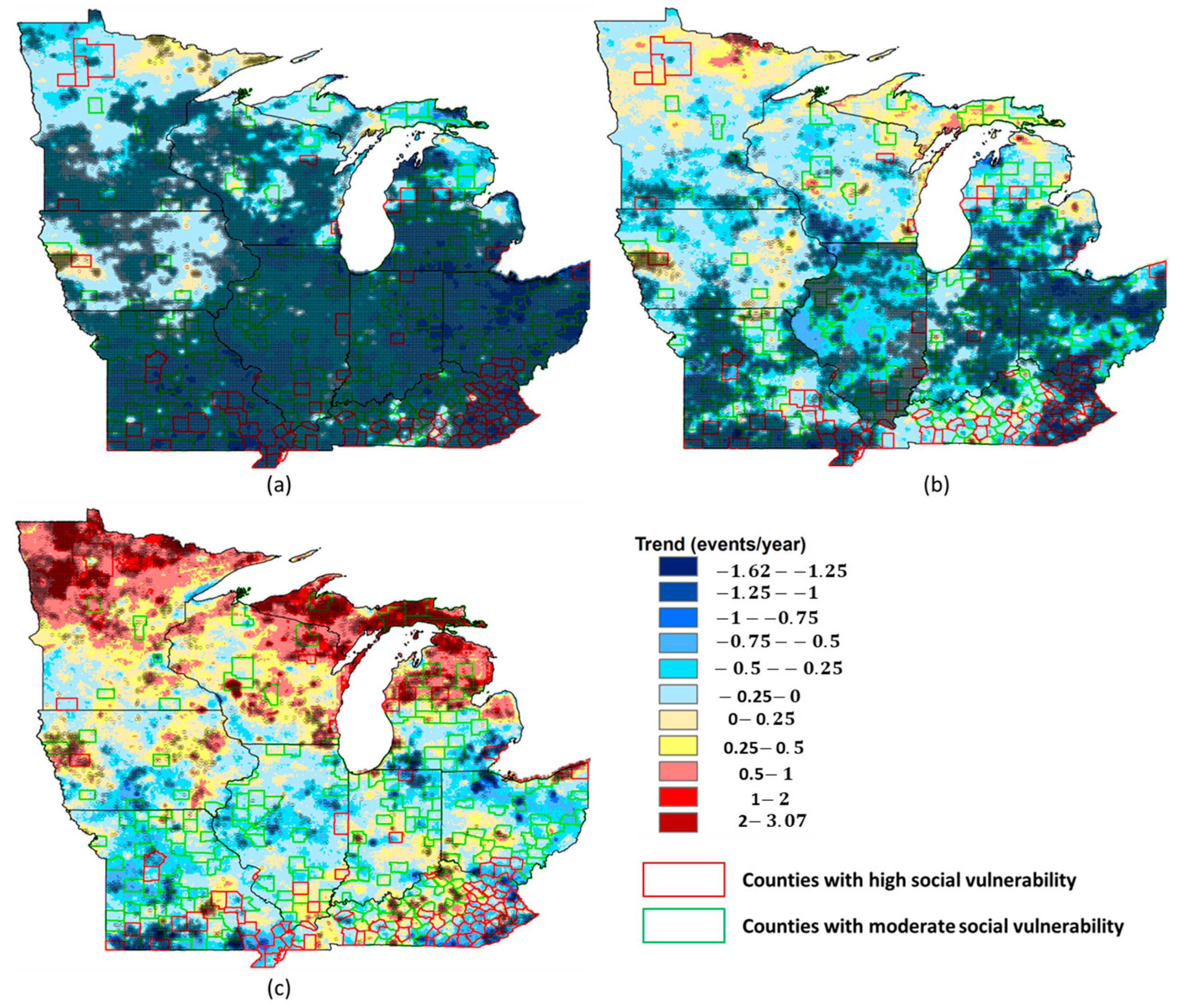
3.2. Trends of Heat Stress Events

A significant increasing trend in DEHI was mostly found in parts of Michigan, Wisconsin (around the lake region), Ohio, and lower parts of Indiana and Kentucky from 1979 to 2021. In contrast, a decreasing trend was noticed in western parts of UMUS (parts of Minnesota, Iowa, and Missouri). The number of grids showing an increasing trend has increased since 1991. The number of grids with a significant increasing trend also went up and was mostly found in parts of Minnesota, Wisconsin, Michigan, Iowa, Illinois, Ohio, and Missouri. Furthermore, the magnitude of the increasing trend in DEHI has been elevated since 2001, mostly in the parts of Iowa, Missouri, Wisconsin, Michigan, Illinois, Indiana, Ohio, and Kentucky (mostly in between 0.75 and 2.25 events/year). A significant increasing trend in DEHI was noticed in a few counties with high social vulnerability, especially in the southern parts of Missouri, Kentucky, Wisconsin, and Michigan, considering the long-term trend (1979–2021) (Figure 2a). However, more counties with high social vulnerability have experienced a significant increasing trend in DEHI since 1991, highlighting the elevated risk of heat-related hazards in recent decades in these areas (Figure 2b,c).

3.3. Spatial Distribution of Extreme Cold Events

The analysis of extreme cold (EC) events over the period 1979–2021 revealed an average annual frequency ranging predominantly between 42 and 44 events per year (Figure 3a). The difference in the average annual EC was found to be mostly negative both between 1991 and 2021 and between 2001 and 2021 compared to 1979–2021 (Figure 3b,c). Interestingly, specific regions within Minnesota, Iowa, and Michigan exhibited a discernible uptick in EC occurrences, with an increase of 2–8 events per year noted since 1991 (Figure 3b). Notably, this trend displayed a notable intensification post-2001, with the frequency of EC events notably escalating (Figure 3c). These EC events are characterized by exceptionally low temperatures and can have significant impacts on agriculture, infrastructure, and human health, especially in socially vulnerable communities. Several counties with high social vulnerability, primarily Iowa, Michigan, and Wisconsin, have been exposed to a higher frequency of EC events since 2001 (Figure 3c).

3.4. Trends of Extreme Cold Events

A significant decreasing trend in extreme cold (EC) events was mostly found throughout the UMUS from 1979 to 2021 (Figure 4a). However, an increasing trend was also noticed in Iowa and northern parts of Minnesota, Michigan, and Wisconsin. The number of grids showing an increasing trend has increased since 1991, mostly in the northern parts of Wisconsin, Michigan, Minnesota, Iowa, and Kentucky (Figure 4b). The number of grids showing an increasing trend has increased significantly since 2001, mostly in Wisconsin, Michigan, northern parts of Minnesota, Iowa, Kentucky, and Ohio. Furthermore, the magnitude of an increasing trend in EC has also elevated since 2001, mostly in Wisconsin, Michigan, and Minnesota (Figure 4c). A significant increasing trend of EC was noticed in a few counties with high social vulnerability, especially in Iowa and Kentucky, considering the long-term trend (1979–2021) (Figure 4a). However, more counties with high to moderate social vulnerability experienced a significant increasing trend of EC since 2001, especially in the northern parts of Minnesota, Wisconsin, and Michigan, as well as in parts of Iowa, Kentucky, Missouri, and Ohio highlighting, elevated risk of extreme cold-related hazard in recent decades in these areas (Figure 4c).

3.5. Hotspot for Compound DEHI and EC Events

An increase in both DEHI and EC events was noticed mainly in the parts of Minnesota, Wisconsin, Michigan, Iowa, Ohio, Kentucky, and Indiana. Although the increasing trends were mainly statistically insignificant, there were a few grids in Michigan, Iowa, Wisconsin, Ohio, and Kentucky, where the increasing trends were statistically significant for both DEHI and EC (Figure 5). The increasing trend in DEHI was mostly noticed during the May–September period, whereas the increasing trend in EC was found during the winter season.

4. Discussion

High humidity intensifies the health impacts of extreme heat by impeding the body’s cooling through sweating. The heat index, combining temperature and humidity, reflects how hot it feels. Humidity affects evaporation, which cools the body. High humidity hampers this cooling process, while low humidity helps it. Increased humidity and temperature raise the heat index, directly impacting comfort. Furthermore, heat stress affects different demographic groups unevenly. Vulnerable populations include older adults, those with lower socioeconomic status, individuals living alone, and those with limited access to healthcare and hazard information. Ethnic minorities, people with pre-existing health conditions, and rural residents without air conditioning or green spaces, are also at higher risk [13,14,15,16,17,18,19,20]. Therefore, special focus should be given to the parts of Michigan, Wisconsin (around the Great Lake region), Ohio, lower parts of Indiana, and Kentucky, where an increasing trend of heat stress was noticed. Previous studies also highlighted an increase in temperature extremes in recent decades in the Midwestern United States [35,36]. The counties in these parts with a high social vulnerability index should be prioritized in terms of extreme weather risk management. The increasing trend of heat stress around the Great Lake region can be attributed to an increase in lake surface temperatures, leading to more evaporation adding more water to the atmosphere and leading to high humidity.

Both extreme heat stress and cold temperatures can put a lot of demand pressure on the power grid systems. Extreme temperatures significantly impact power system operations, leading to heightened peak loads and diminished transmission and generation capacity. Prolonged temperature extremes can lead to a rise in cooling- or heating-related electricity demand, causing unusually high and prolonged peak loads, often exceeding regular levels. Furthermore, extremely high temperatures can decrease transmission line capacity, strain the power grid, and impair gas turbine efficiency and capacity, potentially causing severe operational issues due to supply shortages. Moreover, stationary high-pressure zones during prolonged heat stress can lead to calm surface winds, reducing wind generation.

The findings of the current study can lay the foundation for future research. For example, an increase in both heat stress and extreme cold events can lead to an increase in energy demand. Moreover, it can have an even more profound impact, with both heat stress and extreme cold events indicating an increasing trend. Therefore, the impact on power grids in these regions can be investigated. In the present study, daytime heat stress events are analyzed. Therefore, nighttime heat stress, including compound day and nighttime heat stress events, especially in the socially vulnerable counties, can be explored in the future.

The research presented here aims to guide stakeholders in making well-informed decisions about directing cooling, as well as heating, resources to vulnerable communities, fostering a more sustainable and fair adaptation to a changing climate. For instance, a straightforward increase in the use of inefficient air conditioning or heating systems may lead to higher electricity or gas demand in cities, which will eventually lead to more greenhouse gas emissions. In contrast, implementing heat mitigation strategies, such as urban green spaces, offers a more sustainable way to reduce heat-related risks. Moreover, the adoption of heat management tactics can equip communities to address heat- or cold-related challenges effectively. These measures encompass early heat or cold alert systems, emergency preparedness, the establishment of cooling or heating facilities, and the assurance of dependable cooling or heating resources.

Future research should explore how projected climate-change scenarios will impact heat stress and extreme cold events, particularly in socially vulnerable counties. By examining various climate-change projections, researchers can better anticipate how shifts in temperature and humidity patterns may influence the frequency, intensity, and duration of these events. Understanding these effects is crucial for developing adaptation strategies tailored to the specific needs of vulnerable populations. Additionally, investigating the implications of increased energy demand resulting from more frequent extreme weather events is essential for ensuring the resilience of power grid systems. Expanding research to include nighttime heat stress and compound day–night events, especially in vulnerable areas, will also provide a more comprehensive understanding of risks. Nighttime heat stress poses unique challenges, as it can disrupt sleep patterns and exacerbate health risks for vulnerable populations, such as the elderly and those with pre-existing medical conditions. By analyzing these additional dimensions of heat stress, researchers can gain a more comprehensive understanding of the risks posed by extreme temperatures and develop targeted interventions to mitigate their impact. Incorporating community perspectives and local knowledge into research efforts can enhance the relevance and effectiveness of adaptation strategies. Overall, integrating climate projections, energy infrastructure analysis, and community engagement will enable the development of robust and equitable adaptation measures to address the challenges of a changing climate.

5. Conclusions

Addressing the implications of extreme temperature events is vital in the context of climate change, which impacts public health and strains energy infrastructure. This study critically assesses deadly heat stress and extreme cold events in the Upper Midwestern United States from 1979 to 2021, emphasizing their substantial impact on socially vulnerable communities. The findings indicated that, between 1979 and 2021, the northern regions of the Upper Midwestern United States (UMUS) experienced a comparatively lower average annual frequency of daytime extreme heat stress events than their southern counterparts. Notably, there was a significant upward trend in daytime extreme heat stress in specific areas, including parts of Michigan, Wisconsin (around the lake region), Ohio, and the lower regions of Indiana and Kentucky. The study also revealed a significant decrease in extreme cold events across the UMUS during the same period. However, there was an increasing trend in Iowa and the northern parts of Minnesota, Michigan, and Wisconsin. This suggests that these areas, especially the counties in these parts with a high social vulnerability index, should be prioritized in terms of extreme weather risk management. The findings offer crucial insights into comprehending the risks associated with extreme temperature events, particularly for socially vulnerable communities. This understanding is essential for tailoring effective interventions and building resilience in the context of increasing climate-related challenges. Moreover, the results can assist stakeholders in making informed decisions about allocating resources for cooling and heating to vulnerable communities, thereby promoting a more sustainable and equitable approach to adapting to a changing climate.

References

1. Khan, M.; Bhattarai, R.; Chen, L. Elevated Risk of Compound Extreme Precipitation Preceded by Extreme Heat Events in the Upper Midwestern United States. Atmosphere 2023, 14, 1440. [Google Scholar] [CrossRef]
2. Khan, M.; Chen, L.; Markus, M.; Bhattarai, R. A probabilistic approach to characterize the joint occurrence of two extreme precipitation indices in the upper Midwestern United States. JAWRA J. Am. Water Resour. Assoc. 2023, 60, 529–542. [Google Scholar] [CrossRef]
3. Angelil, O.; Stone, D.; Wehner, M.; Paciorek, C.J.; Krishnan, H.; Collins, W. An independent assessment of anthropogenic attribution statements for recent extreme temperature and rainfall events. J. Clim. 2017, 30, 5–16. [Google Scholar] [CrossRef]
4. Vose, R.S.; Easterling, D.R.; Kunkel, K.E.; LeGrande, A.N.; Wehner, M.F. Temperature changes in the United States. In Climate Science Special Report: Fourth National Climate Assessment; Wuebbles, D.J., Fahey, D.W., Hibbard, K.A., Dokken, D.J., Stewart, B.C., Maycock, T.K., Eds.; Global Change Research Program: Washington, DC, USA, 2017; Volume I, pp. 185–206. [Google Scholar] [CrossRef]
5. Allan, R.P.; Hawkins, E.; Bellouin, N.; Collins, B. IPCC, 2021: Summary for Policymakers; IPCC: Geneva, Switzerland, 2021. [Google Scholar]
6. Basu, R. High ambient temperature and mortality: A review of epidemiologic studies from 2001 to 2008. Environ. Health 2009, 8, 40. [Google Scholar] [CrossRef]
7. Basu, R.; Samet, J.M. Relation between elevated ambient temperature and mortality: A review of the epidemiologic evidence. Epidemiol. Rev. 2002, 24, 190–202. [Google Scholar] [CrossRef] [PubMed]
8. Mora, C.; Dousset, B.; Caldwell, I.R.; Powell, F.E.; Geronimo, R.C.; Bielecki, C.R.; Counsell, C.W.W.; Dietrich, B.S.; Johnston, E.T.; Louis, L.V.; et al. Global risk of deadly heat. Nat. Clim. Chang. 2017, 7, 501–506. [Google Scholar] [CrossRef]
9. Jones, B.; O’Neill, B.C.; McDaniel, L.; McGinnis, S.; Mearns, L.O.; Tebaldi, C. Future population exposure to US heat extremes. Nat. Clim. Chang. 2015, 5, 652–655. [Google Scholar] [CrossRef]
10. National Weather Service (NWS). Available online: https://www.weather.gov/hazstat/ (accessed on 5 January 2024).
11. CDC Report on Heat-Related Illness. Available online: https://www.cdc.gov/Mmwr/preview/mmwrhtml/mm6331a1.htm (accessed on 20 August 2023).
12. Fowler, D.R.; Mitchell, C.S.; Brown, A.; Pollock, T.; Bratka, L.A.; Paulson, J.; Noller, A.C.; Mauskapf, R.; Oscanyan, K.; Vaidyanathan, A.; et al. Heat-related deaths after an extreme heat event—Four states, 2012, and United States, 1999–2009. Morb. Mortal. Wkly. Rep. 2013, 62, 433. [Google Scholar]
13. Naughton, M.P.; Henderson, A.; Mirabelli, M.C.; Kaiser, R.; Wilhelm, J.L.; Kieszak, S.M.; Rubin, C.H.; McGeehin, M.A. Heat-related mortality during a 1999 heat wave in Chicago. Am. J. Prev. Med. 2002, 22, 221–227. [Google Scholar] [CrossRef]
14. Fouillet, A.; Rey, G.; Laurent, F.; Pavillon, G.; Bellec, S.; Guihenneuc-Jouyaux, C.; Clavel, J.; Jougla, E.; Hémon, D. Excess mortality related to the August 2003 heat wave in France. Int. Arch. Occup. Environ. Health 2006, 80, 16–24. [Google Scholar] [CrossRef]
15. Rey, G.; Fouillet, A.; Bessemoulin, P.; Frayssinet, P.; Dufour, A.; Jougla, E.; Hémon, D. Heat exposure and socioeconomic vulnerability as synergistic factors in heat-wave-related mortality. Eur. J. Epidemiol. 2009, 24, 495–502. [Google Scholar] [CrossRef] [PubMed]
16. O’Neill, M.S.; Zanobetti, A.; Schwartz, J. Modifiers of the temperature and mortality association in seven U.S. cities. Am. J. Epidemiol. 2003, 157, 1074–1082. [Google Scholar] [CrossRef]
17. Stafoggia, M.; Forastiere, F.; Agostini, D.; Caranci, N.; de’Donato, F.; Demaria, M.; Michelozzi, P.; Miglio, R.; Rognoni, M.; Russo, A.; et al. Factors affecting in-hospital heat-related mortality: A multi-city case-crossover analysis. J. Epidemiol. Community Health 2008, 62, 209–215. [Google Scholar] [CrossRef]
18. Semenza, J.C.; Rubin, C.H.; Falter, K.H.; Selanikio, J.D.; Flanders, W.D.; Howe, H.L.; Wilhelm, J.L. Heat-related deaths during the July 1995 heat wave in Chicago. N. Engl. J. Med. 1996, 335, 84–90. [Google Scholar] [CrossRef]
19. Curriero, F.C.; Heiner, K.S.; Samet, J.M.; Zeger, S.L.; Strug, L.; Patz, J.A. Temperature and mortality in 11 cities of the eastern United States. Am. J. Epidemiol. 2002, 155, 80–87. [Google Scholar] [CrossRef]
20. Tan, J.; Zheng, Y.; Song, G.; Kalkstein, L.S.; Kalkstein, A.J.; Tang, X. Heat wave impacts on mortality in Shanghai, 1998 and 2003. Int. J. Biometeorol. 2007, 51, 193–200. [Google Scholar] [CrossRef] [PubMed]
21. CDC. Available online: https://www.weather.gov/ama/heatindex (accessed on 10 January 2024).
22. EPA. Available online: https://climatechange.chicago.gov/climate-impacts/climate-impacts-human-health#ref1 (accessed on 15 January 2024).
23. IPCC. Managing the Risks of Extreme Events and Disasters to Advance Climate Change Adaptation. A Special Report of Working Groups I and II of the Intergovernmental Panel on Climate Change; Field, C.B., Barros, V., Stocker, T.F., Qin, D., Dokken, D.J., Ebi, K.L., Mastrandrea, M.D., Mach, K.J., Plattner, G.-K., Allen, S.K., Tignor, M., Midgley, P.M., Eds.; Cambridge University Press: Cambridge, UK; New York, NY, USA, 2012; 582p, Available online: https://www.ipcc.ch/site/assets/uploads/2018/03/SREX_Full_Report-1.pdf (accessed on 25 October 2023).
24. Reid, C.E.; O’Neill, M.S.; Gronlund, C.J.; Brines, S.J.; Brown, D.G.; Diez-Roux, A.V.; Schwartz, J. Mapping community determinants of heat vulnerability. Environ. Health Perspect. 2009, 117, 1730–1736. [Google Scholar] [CrossRef] [PubMed]
25. Rinner, C.; Patychuk, D.; Jakubek, D.; Nasr, S.; Bassil, K.L.; Campbell, M. Development of a Toronto-Specific, Spatially Explicit Heat Vulnerability Assessment: Phase, I; Toronto Public Health: Toronto, ON, Canada, 2009. [Google Scholar]
26. Johnson, D.P.; Stanforth, A.; Lulla, V.; Luber, G. Developing an applied extreme heat vulnerability index utilizing socioeconomic and environmental data. Appl. Geogr. 2012, 35, 23–31. [Google Scholar] [CrossRef]
27. Reid, C.E.; Mann, J.K.; Alfasso, R.; English, P.B.; King, G.C.; Lincoln, R.A.; Margolis, H.G.; Rubado, D.J.; Sabato, J.E.; West, N.L.; et al. Evaluation of a heat vulnerability index on abnormally hot days: An environmental public health tracking study. Environ. Health Perspect. 2012, 120, 715–720. [Google Scholar] [CrossRef]
28. Harlan, S.L.; Declet-Barreto, J.H.; Stefanov, W.L.; Petitti, D.B. Neighborhood effects on heat deaths: Social and environmental predictors of vulnerability in Maricopa County, Arizona. Environ. Health Perspect. 2013, 121, 197–204. [Google Scholar] [CrossRef]
29. Maier, G.; Grundstein, A.; Jang, W.; Li, C.; Naeher, L.P.; Shepherd, M. Assessing the performance of a vulnerability index during oppressive heat across Georgia, United States. Weather. Clim. Soc. 2014, 6, 253–263. [Google Scholar] [CrossRef]
30. Abatzoglou, J.T. Development of gridded surface meteorological data for ecological applications and modelling. Int. J. Climatol. 2013, 33, 121–131. [Google Scholar] [CrossRef]
31. Centers for Disease Control and Prevention/Agency for Toxic Substances and Disease Registry/Geospatial Research, Analysis and Services Program. CDC/ATSDR Social Vulnerability Index, 2020. Database US. Available online: https://www.atsdr.cdc.gov/placeandhealth/svi/data_documentation_download.html (accessed on 15 October 2023).
32. Steadman, R.G. The assessment of sultriness. Part I: A temperature-humidity index based on human physiology and clothing science. J. Appl. Meteor. 1979, 18, 861–873. [Google Scholar] [CrossRef]
33. Kendall, M.G. Rank Correlation Methods; Griffin: Duxbury, MA, USA, 1948. [Google Scholar]
34. Mann, H.B. Nonparametric tests against trend. Econometrica. J. Econom. Soc. 1945, 13, 245–259. [Google Scholar]
35. Ning, L.; Bradley, R.S. Influence of eastern Pacific and central Pacific El Niño events on winter climate extremes over the eastern and central United States. Int. J. Clim. 2015, 35, 4756–4770. [Google Scholar] [CrossRef]
36. Mutiibwa, D.; Vavrus, S.J.; McAfee, S.A.; Albright, T.P. Recent spatiotemporal patterns in temperature extremes across conterminous United States. J. Geophys. Res. Atmos. 2015, 120, 7378–7392. [Google Scholar] [CrossRef]
Figure 1. Study area of the Upper Midwestern United States (UMUS), including Illinois (IL), Missouri (MO), Kentucky (KY), Indiana (IN), Ohio (OH), Iowa (IA), Minnesota (MN), Wisconsin (WI) and Michigan (MI).
Atmosphere 15 00614 g001
Figure 2. Temporal trend of daytime extreme heat stress (DEHI) during (a) 1979–2021, (b) 1991–2021, and (c) 2001–2021. The grids with shading represent the grids with significant trends at a 95% significance level. The boundaries of counties with moderate and high social vulnerability are shown green and red, respectively.
Atmosphere 15 00614 g002
Figure 3. (a) Spatial trend of average annual extreme cold (EC) days from 1979 to 2021. Spatial trend of difference in average annual EC in the Upper Midwestern United States (UMUS) in between (b) the ranges 1991–2021 and 1979–2021; and (c) the ranges 2001–2021 and 1979–2021. The boundaries of counties with moderate and high social vulnerability are shown in green and red, respectively.
Atmosphere 15 00614 g003
Figure 4. Temporal trend of extreme cold (EC) days during (a) 1979–2021, (b) 1991–2021, and (c) 2001–2021. The grids with shading represent the grids with significant trends at a 95% significance level. The boundaries of counties with moderate and high social vulnerability are shown in green and red, respectively.
Atmosphere 15 00614 g004
Figure 5. Spatial distribution of the trend of compound daytime extreme heat stress (DEHI) and extreme cold (EC) events in the Upper Midwestern United States (UMUS) from 2000 to 2021. The boundaries of counties with moderate and high social vulnerability are shown in green and red, respectively.
Atmosphere 15 00614 g005
Disclaimer/Publisher’s Note: The statements, opinions and data contained in all publications are solely those of the individual author(s) and contributor(s) and not of MDPI and/or the editor(s). MDPI and/or the editor(s) disclaim responsibility for any injury to people or property resulting from any ideas, methods, instructions or products referred to in the content.