Sensitivity of the Intensity and Structure of Tropical Cyclones to Tropospheric Stability Conditions

Abstract

The intensity of tropical cyclones (TCs) is controlled by their environmental conditions. In addition to the sea surface temperature, tropospheric temperature lapse rate and tropopause height are highly variable. This study investigates the sensitivity of the intensity and structure of TCs to environmental static stability with a fixed sea surface temperature by conducting a large ensemble of axisymmetric numerical experiments in which tropopause height and tropospheric temperature lapse rate are systematically changed based on the observed environmental properties for TCs that occurred in the western North Pacific. The results indicate that the intensity of the simulated TCs changes more sharply with the increase in the temperature lapse rate than with the increase in the tropopause height. The increases in the intensity of TCs are 1.3–1.9 m s⁻¹ per 1% change of the lapse rate and 0.1–0.5 m s⁻¹ per 1% change of the tropopause height. With the increase in the intensity of TCs, supergradient wind at low levels and double warm core structures are evident. Specifically, the formation of the warm core at the lower levels is closely tied with the intensification of TCs, and the temperature excess of the lower warm core becomes larger in higher lapse rate cases.

1. Introduction

The development of tropical cyclones (TCs) is controlled by their environmental conditions. Diagnosing and predicting the maximum intensity achievable during the lifetime of TCs are important to forecasting severe weather and hazards due to TCs. Gray [1] statistically identified environmental conditions favorable for the development of TCs, and indicated that TCs favorably develop under conditions with warm SST, convective instability in the lower troposphere, positive relative vorticity at low-levels, weak vertical wind shear, high relative humidity at middle-levels, and significant planetary vorticity. Among these environmental factors, SST and convective instability play a key role in determining the intensity of TCs.

There have been a number of studies of how the maximum intensity of TCs is determined (e.g., [2,3,4,5,6,7]). Emanuel [2,3] put forth a maximum potential intensity (MPI) theory based on the proposition that TC circulation can be regarded as a Carnot heat cycle. Based on Emanuel’s theory, Bister and Emanuel [8] presented an equation of MPI which indicates that the maximum wind speed is determined by SST, outflow temperature, and surface enthalpy flux. Bister and Emanuel [9] updated the MPI equation to show that the surface enthalpy flux term can be replaced with convective available potential energy (CAPE). In this way, the atmospheric stability conditions play a role in determining the intensity of TCs.

The understanding of the impacts of the environmental conditions such as SST, outflow temperature, and relative humidity, on the intensity of TCs has steadily progressed. On the other hand, there have not been many studies on how atmospheric stability such as temperature lapse rate affects the development of TCs. Hendricks et al [10] examined the environmental conditions for the intensity changes of TCs in the western North Pacific and the North Atlantic and found that the rate of intensification of the TCs in the both basins is not critically dependent on SST. Particularly in the western North Pacific, rapidly intensifying TCs occur when environmental instability is high. Stovern and Ritchie [11] investigated the sensitivity of the TC structure to the temperature conditions and found that a warmer environment with a higher CAPE is important for the rapid development of a more intense inner-core precipitation and wind, whereas a colder environment with a lower CAPE leads to a broader inner and outer core of convection. However, in their study [11], although the temperature in the entire atmosphere was uniformly warmed or cooled by a 1 °C increment, the temperature lapse rate was unchanged. Some studies focused on how the temperature profile in the upper troposphere and lower stratosphere affects the intensity and structure of TCs [12,13,14], but these studies did not change the temperature in the entire troposphere. There are also some studies that investigated the effects of tropospheric stability on TCs in the context of the impacts of climate change. Shen et al. [15] and Tuleya et al. [16] investigated the sensitivity of the TC intensity to temperature lapse rate as well as SST and showed that the simulated TCs can intensify as the atmosphere becomes unstable under the same SST. However, how the impacts of the lapse rate appeared on the structure of TCs were not clearly examined in their studies. Hill and Lackmannn [17] examined the influence of the vertical structure of future atmospheric conditions on TCs from the predictions of multiple general circulation models by conducting sensitivity experiments with changes in resolution, physical processes and future climate conditions. They showed that the TC intensity increases in almost all the future conditions irrespective of the resolution and physical processes. Kanada et al. [18] examined changes in the intensity and structure of Typhoon Vera (1959), a category-five storm that occurred in September 1959 and landed in central Japan, under environments of future global warming, by conducting pseudo-global warming (PGW) experiments with different non-hydrostatic models. In the PGW experiment, the background states in a future climate are produced by adding warming increments to past analysis fields [19,20]. Kanada et al. [18] showed that Typhoon Vera in the future conditions under the RCP 8.5 scenario intensifies mainly owing to the increase in water vapor content and SST in spite of the more-stable troposphere and also showed that the updrafts within the eyewall of Typhoon Vera intensify and reach higher levels under the future conditions.

One of the advantages of the studies by Hill and Lackmann [17] and Kanada et al. [18] is the use of non-hydrostatic models that can explicitly represent TC-scale circulations. However, there are some disadvantages of these studies: they used three-dimensional models with large computational costs, and the grid spacings employed in their studies were not sufficient for resolving individual convective clouds. Specifically, Hill and Lackmann [17] employed a horizontal grid spacing of 6 km for an ensemble of experiments, and Kanada et al. [18] used a grid spacing of 5 km. Such grid spacings may be in a cloud-permitting range and are not able to explicitly resolve individual convection. Hill and Lackmann [17] used a 2-km grid spacing in a nested domain from the 6-km-grid domain, but the number of the 2-km-grid experiments is greatly limited. Although the cloud-permitting resolution is at least desirable to capture quantitatively the intensity and structure of TCs, the results may include a number of uncertainties. Thus, how the stability quantitatively affects the intensity and structure of TCs has not been comprehensively investigated. The understanding of the effect of stability should be important not only from a climate projection point of view but also from a weather prediction point of view.

In considering the effects of static stability on convection in general, the temperature lapse rate determines the amount of CAPE and thus controls the updraft intensity, thereby affecting the degree of the organization of mesoscale convective systems (MCSs) [21,22,23,24]. Under a lower lapse rate condition, the buoyancy is weaker, and thus the updraft is weaker, resulting in a lower degree of MCS organization. Another point is that, even in a lower lapse rate condition, the increase in the tropopause height will lead to a higher level of neutral buoyancy and hence add a small amount of CAPE [25]. Furthermore, according to the MPI theory of TCs [2,3], the increase in the tropopause height corresponds to the decrease in outflow temperature, potentially enhancing the maximum intensity of TCs. Therefore, the effects of the tropospheric stability conditions are of scientific interest for the understanding of the TC intensity.

The purpose of this study is to quantify the impacts of environmental static stability on the intensity and structure of TCs by conducting a large number of numerical experiments with the use of an axisymmetric, non-hydrostatic model configured in environments with stability conditions systematically changed. In particular, we investigate the intensity and structure of TCs during their mature stage by examining the vertical circulation and eyewall convection. By using a low-cost, two-dimensional, axisymmetric model, we are able to perform a large number of sensitivity experiments in which the tropospheric temperature lapse rate and the tropopause height are systematically changed, thereby demonstrating quantitatively the sensitivity of the TC intensity to the lapse rate and the tropopause height, and indicating high reliability to the results.

2. Numerical Model and Experimental Design

2.1. Numerical Model

The present study uses the axisymmetric version of Cloud Model version 1, release 19 (CM1) developed by Bryan and Fritsch [26]. CM1 is a non-hydrostatic, fully compressible model and has been utilized for the idealized simulations of TCs in a number of studies (e.g., [6,7,12,27]).

The model settings are determined with reference to the previous studies of Bryan and Rotunno [6] and Bryan [27] who examined the TC dynamics under an axisymmetric framework. The domain covers 1500 km in the radial and 25 km in the vertical direction, and the grid spacings are 1 km in the radial direction and 250 m in the vertical direction. The central axis of the TC is set as a lateral boundary having an axisymmetric condition, while at the outside lateral boundary a rigid, free slip wall condition is imposed. The top boundary is a free slip, with a Rayleigh damping layer being applied above the 20 km height. The surface boundary is assumed to be the ocean. To develop a TC, a Rankine-type vortex used in Rotunno and Emanuel [4] is embedded in the domain at the initial time. This vortex is assumed to be in a state of gradient and hydrostatic balance and has the maximum wind speed of 12 ${\mathrm{m}\mathrm{s}}^{-1}$ and the radius of the maximum wind of 100 km.

In order to simplify the interpretation of physical processes related to the TC development, we choose the simplest physical schemes possible. A Kessler-type warm-rain scheme was selected for cloud microphysics. For atmospheric radiation, the Newtonian cooling with the rate of 2 K day⁻¹ was applied to mimic radiative cooling, following the idea of Rotunno and Emanuel [4]. Turbulence mixing was parameterized with a Smagorinsky-type scheme in which the horizontal and vertical length scales (l_h and l_v, respectively) were set according to Bryan [27]. Because the SST in this study was set to a higher value (303.5 K) than used in Bryan [27], l_h was changed from 1000 m to 1500 m in order to prevent TCs from excessive development. Note that the SST value was determined from the analysis of the environment for Typhoon Vera (1959), which will be described in detail in the next subsection. The surface exchange coefficients C_k and C_d for enthalpy and momentum, respectively, were set as constant values: C_k = 1.2 × 10⁻³, C_d = 2.4 × 10⁻³. Bryan [27] showed that the intensity of simulated TCs based on these exchange coefficients is in the best agreement with the observation, and therefore we also used these values. The computational domain was assumed to be a f-plane with $f=5\times {10}^{-5} {\mathrm{s}}^{-1}$. All experiments were integrated in time for 250 h.

2.2. Environmental Stability Diagnosed from Reanalysis Data

The initial vertical profiles of temperature and humidity in the present experiments were generated with reference to the environmental conditions when Typhoon Vera (1959) recorded the maximum intensification rate during 24 h (at the time 0000 UTC, 22 September 1959). We used the best track dataset of Joint Typhoon Warning Center (JTWC) in order to obtain information on the position and intensity of Typhoon Vera, and used the Japanese 55-year Reanalysis (JRA-55; Kobayashi et al. [28]) for analyzing the environmental conditions. We took horizontal averages of temperature, relative humidity, and geopotential height within the 10° by 10° area centered at the typhoon center and defined these averaged fields as the horizontally uniform, initial state for the control experiment (referred to as CTL). Note that the layer from the surface to the depth of 1.5 km is regarded as a boundary layer, in which the temperature lapse rate was set to a constant value (i.e., 6.41 K km⁻¹) and the relative humidity was set to an area-average value at each level. In the CTL experiment as well as the sensitivity experiments described in the following, we assume that the initial atmosphere is at rest.

In order to set the vertical profiles of temperature and humidity in the sensitivity experiments, we examined the environmental conditions around TCs in the western North Pacific during the period from 1979 to 2014. The environments for 1068 TCs occurred in the western North Pacific during this period as well as for Typhoon Vera (1959) were chosen. The environmental conditions for these TCs were determined by computing the horizontally averaged field as was done when creating the vertical profiles for the CTL experiment. The relationships between the environmental variables and the maximum intensity of TCs are shown in Figure 1. The maximum intensity of the observed TCs tends to increase with the SST increase (Figure 1a). A tendency for the increase in the TC maximum intensity with the decrease in the tropopause temperature is also seen (Figure 1b). The influence of static stability on the intensity of TCs is also seen: the maximum intensity tends to increase as temperature lapse rate or CAPE increases (Figure 1c,d). As JRA-55 has a coarse vertical resolution in the layer near the tropopause, the values of the tropopause height are not continuous but are instead discrete; hence, the relationship with intensity is difficult to be identify (Figure 1e). It is clear that the development of TCs is prevented by the strengthening of the vertical wind shear in the layer between 850 and 200 hPa (Figure 1f).

In Figure 1, the environment when Typhoon Vera (1959) developed is also indicated. The environmental conditions of Typhoon Vera is characterized by remarkably high SST, a large temperature lapse rate, and medium values of tropopause temperature and CAPE. We regard this environmental condition of Typhoon Vera as CTL.

Table 1. The values of the environmental parameters obtained from the JRA-55 analysis. The 1st percentile, median, and 99th percentile values are indicated.

Parameters	Observations
	1%	Median	99%
Γ [K km−1]	6.22	6.64	6.93
Ht [m]	15,230	16,591	16,723
To [K]	187.3	193.2	204.2
CAPE [J kg−1]	638	2927	4816
SST [K]	299.3	302.1	303.4

summarizes the statistics of some environmental properties obtained from the above analysis of the JRA-55 data. Here, the tropopause height H_t is defined as the lowest level at which the temperature lapse rate Γ becomes less than 3 K km⁻¹ [29] (note here that in the original WMO definition the threshold lapse rate is 2 K km⁻¹, but in this study we employ a stricter threshold), and the temperature at that level is defined as the tropopause temperature T_o. In setting the initial conditions in the numerical experiments, the values indicated in Table 1 are regarded as the reference.

2.3. Experimental Design

Based on the analysis described in the previous subsection, we determined the initial stability conditions for the sensitivity experiments in which the tropospheric temperature lapse rate and the tropopause height are systematically varied. The procedure is described as follows.

First, the values of H_t and T_o in CTL are set to be 15,375 m and 197.7 K, respectively.

The vertical profiles of temperature above 1.5-km height in the sensitivity experiments with the tropopause temperature varied were generated by multiplying a factor to the temperature at each height in order for the tropopause temperature to be set in the increment of 1 K. In this study, the temperature lapse rate between the 1.5-km height and the tropopause is hereinafter referred to as Γ. The temperature lapse rates above the tropopause height were not changed from the CTL profile.

Furthermore, the tropopause height H_t was lowered or elevated at an increment of 250 m from the height used in CTL. In elevating the tropopause, we extrapolated the temperature profile by keeping the temperature lapse rate at the tropopause in CTL.

The values of T_o and H_t were varied in the ranges from the −2 K to +6 K and from −1 km to +1 km, respectively, with respect to the values of CTL. These ranges are based on the analysis of JRA-55 as shown in Figure 1 and Table 1. In all the experiments, the vertical distribution of relative humidity was set to be the same as in CTL, and SST was set to the area-averaged value of 303.5 K.

Table 2. The values of the environmental parameters. Indicated are the values in the CTL and sensitivity experiments, obtained from the JRA-55 analysis, and in the pseudo-global warming (PGW) experiment of Kanada et al. [18]. For the sensitivity experiments, the minimum and maximum values are indicated.

Parameters	CTL	Sensitivity Experiment		PGW Mean
		Min.	Max.
Γ [K km−1]	6.75	6.25	6.92	6.34
Ht [m]	15,375	14,375	16,375	16,875
To [K]	197.7	188.3	210.9	197.0
CAPE [J kg−1]	3091	1611	3769	4063
SST [K]	303.5			306.4

summarizes the parameters set in the experiments. The temperature profiles are shown in Figure 2. In addition, plotted in Figure 2 is the vertical profile for the PGW experiments used in Kanada et al. [18] as a reference.

From Table 2, we can see that the Γ value of CTL is close to the median value of the observations (see Table 1), and that SST of CTL is remarkably high and exceeds the 99th percentile value of the observations (see Table 1). Since we set the boundary-layer temperature profile as well as the tropospheric relative humidity to be unchanged among all the experiments, the value of CAPE should increase in proportion to Γ; this relationship is seen in Table 2. It is noted that the tropospheric temperature lapse rate under the PGW condition used in Kanada et al. [18] is very stable compared with the profiles defined in the sensitivity experiments (Table 2, Figure 2). A total of 81 numerical experiments are conducted in this study.

One may argue that the latent heat releases from ice microphysical processes should be included in order to give credence to the physical reality of the simulated TCs even under idealized conditions. To respond to this concern, we also performed another set of numerical experiments with an ice-phase processes parameterization [30]. Although the main results are presented from the experiments with Kessler’s warm rain parameterization, the comparison of these results with those with the warm-rain and ice-phase microphysics parameterization is discussed in Section 4.

3. Results

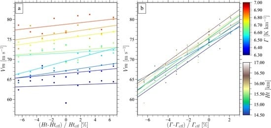
3.1. Responses of TC Intensity to Tropospheric Stability

Here we describe the responses of the intensity and structure of the simulated TCs to the vertical profile of temperature. First, the overall evolution of the simulated TCs is demonstrated. Figure 3 shows the temporal change in the intensity of TCs simulated in CTL and all the sensitivity experiments in terms of maximum wind speed and surface central pressure. Here, the maximum wind speed V_m is defined as the maximum tangential wind at the 10-m height. In CTL, the vortex developed rapidly after the simulated time, t = 40 h, and finished the rapidly intensifying period at about t = 80 h, reaching the maximum intensity at around t = 130 h. After this time, the TC weakened slightly and reached an equilibrium state at around t = 150 h, which continues until the end of the simulation. The maximum wind speed and the central pressure during this equilibrium state are in good agreement with the maximum intensity of Typhoon Vera (1959) within the range of maximum intensities recorded by both Japan Meteorological Agency (JMA) and JTWC best-track data. Thus, CTL reproduces the actual intensity of Typhoon Vera in spite of the idealized experimental setup.

In the sensitivity experiments, the rate of intensification and the intensity in the equilibrium state of the simulated TCs vary around those obtained in CTL. The intensity differences among the members at the end of the time integration are 30 m s⁻¹ for the maximum wind speed and 78 hPa for the central pressure. In spite of these differences, the TCs simulated in the sensitivity experiments also reached their equilibrium states after t = 150 h. Thus, the intensity of the simulated TCs averaged during the equilibrium state (i.e., the time period t = 150–250 h) was used to examine the influences of the static stability and the tropopause height. The mean maximum wind speed averaged in the equilibrium time period was denoted as V_m*.

The sensitivity of the maximum intensity V_m* of the simulated TCs to the tropopause height and the tropospheric temperature lapse rate obtained from all the experiments is shown in Figure 4. The tropopause height and the temperature lapse rate on the horizontal axes of Figure 4 are indicated by the differences from the CTL values, normalized by the CTL values and indicated as percentages. From Figure 4a, we can see that in some Γ cases V_m* increases with the increase in H_t while in other cases V_m* does not correlate with the increase in H_t. The slopes of the linear-fitting lines of the relationship of V_m* to H_t ranges from 0.1 to 0.5 m s⁻¹ per 1% change of H_t. On the other hand, the intensity of the TCs increases sharply with the increase in Γ in all the H_t cases (Figure 4b). In this series of the experiments, the slope of the linearly fitted lines of the relationship of V_m* to Γ ranges between 1.3 and 1.9 m s⁻¹ per 1% change of Γ. The results shown in Figure 4 indicate that the intensity of the TCs is more sensitive to Γ than to H_t.

Since the intensity of the TCs is closely tied with the structure of the TCs, the structure of the TCs will also change in response to the differences of Γ and H_t. The radius and height cross sections during the equilibrium states are shown in Figure 5 for CTL and selected two cases with H_t changed but Γ unchanged at the CTL value, and are shown in Figure 6 for CTL and two cases with Γ changed but H_t unchanged at the CTL value. In order to account for the temporal changes in the radial size of the TC core, the radius on the horizontal axis was normalized by the radius of the maximum wind at the 2-km height (RMW_{2 km}) at each time. In CTL (Figure 5b), the updraft in the eyewall, located around the normalized radius of 1, has two peaks: one at the lower level (around the 2-km height) and the other at the upper level (around the 10-km height). An inflow layer with a maximum value of 30 m s⁻¹ develops in the boundary layer, and just above this inflow layer a concentrated region of an outflow with the maximum value of 15 ${\mathrm{m}\mathrm{s}}^{-1}$ appears. The intensity of the upper-level outflow located near the tropopause is about 25 m s⁻¹. The standard deviation of the updraft is higher in the upper part of the troposphere in the eyewall region, and there are two maxima in the upper layer (Figure 5e). This indicates that the updraft in the upper layer changes its relative location to RMW_{2 km}; with time, the slope of the updraft and the eyewall convection changes from upright to more slanted. On the other hand, the variability of the updraft in the lower level is low, which suggests that the structure of the low-level updraft is well established during the equilibrium state.

In the selected sensitivity experiments, the general structure of the secondary circulation is basically the same as in CTL; strong low-level inflow, localized outflow just above the inflow layer, double-peaked updraft in the eyewall, and outflow near the tropopause are seen in Figure 5a,c. There are slight changes in the peak intensities of the radial and vertical winds, but they seem to be minor. Two maxima in the standard deviation of the updraft are also seen, which is related to variation of the eyewall slope (Figure 5d,f). In the experiment in which H_t is lowered by 1 km (Figure 5a), the updraft in the eyewall became weaker than that in CTL, but V_m* did not decrease from the CTL case. On the other hand, in the experiment with H_t elevated by 1 km (Figure 5c), the updraft and the upper-layer outflow appeared to be stronger than those in the CTL case, and V_m* also increased from the CTL value. It is seen that the depth of the eyewall became deeper with the increase in H_t. It is considered that the deeper eyewall slightly strengthens the updraft in the eyewall. From these results, we can find that the increase in the tropopause height leads to the strengthening of the eyewall updraft but does not necessarily lead to the increase in V_m*.

The impacts of the change in the temperature lapse rate on the secondary circulation of TCs are exhibited in Figure 6. The CTL case is also reproduced in Figure 6 for comparison purposes. The low-level inflow, the outflow just above the inflow layer, the eyewall updraft, and the upper-level outflow of the TC, in the case with the more stable conditions, are weaker than those of the CTL (Figure 6a). This structural change is consistent with the reduced intensity of the TC in this stable condition case in terms of V_m*. In contrast, the inflow, the updraft, and the outflows become intensified in the case with the unstable condition (Figure 6c) relative to those in CTL. As far as the standard deviation of the updraft is concerned, there is a single maximum within the eyewall region in the stable conditions case (Figure 6d). In addition, the slope of the updraft in this case seems to be more upright than that of the CTL (compare Figure 6a,c). This indicates that the structure of the updraft in the stable conditions case does not change much in time. On the other hand, the standard deviation of the updraft in the unstable condition case becomes larger than that in CTL especially in the lower layer, in conjunction with intensified inflow-outflow couplet in the lower layer. In this way, the temperature lapse rate seems to have a significant impact on the strength and structure of the secondary circulation of TCs.

Table 3. The mean and standard deviation (std) of maximum winds V_m, central pressure P_min, and radius of maximum winds (RMW) during the equilibrium states. Experiments shown in Figure 5 and Figure 6 are chosen here.

Exp	Vm (m s−1)		Pmin (hPa)		RMW (km)
	Mean	Std	Mean	std	Mean	std
CTL	73.55	2.0	886.4	4.5	23.93	2.32
Htctl—To+6K	59.11	4.6	925.1	9.2	20.89	1.17
Htctl—To−2K	76.70	2.8	875.8	6.7	25.88	2.89
Ht−1km—Toctl	74.32	2.4	883.2	5.7	24.42	1.74
Ht+1km—Toctl	76.94	2.0	875.4	5.7	22.86	2.22

summarizes the statistics of the maximum wind (V_m*), the minimum central pressure (P_min), and the radius of maximum wind (RMW) in the equilibrium states of the simulated TCs shown in Figure 5 and Figure 6. Among the series of the experiments with H_t changed, both P_min and V_m* become stronger when H_t is elevated more than in CTL but do not change consistently when H_t lowered. The value of RMW decreases with the increase in H_t. On the other hand, the results obtained in the experiments with Γ changed demonstrate that the TC intensity becomes stronger and the RMW becomes smaller with increase in Γ; thus, a consistent change in the intensity and size of the TCs appears against the increase in the instability. Among the cases shown, the standard deviations seem not to vary in a consistent manner with the change in H_t or Γ, but overall the values are not significant as compared with the mean values.

3.2. Warm Core Structure and TC Intensity

In this subsection, we examine the influences of Γ and H_t on the warm core of TCs. Figure 7 shows the temporal change of the warm core structure simulated in CTL from t = 75 h to 200 h. Note that the simulated fields were averaged in time for 6 h centered at each specified time, in order to focus on the robust temporal evolution by filtering out the short-time-scale variability around the TC core. At t = 75 h (Figure 7a), the TC forms double warm cores with peaks around the heights of 5 km and 17 km. The intensity of the lower and the upper warm cores gradually increases with time from t = 75 h (when the TC is in developing stage) to t = 125 h (when the TC is at its peak intensity, Figure 7c). After t = 150 h (Figure 7d) until t = 200 h (Figure 7f), the structure of these warm cores seems to be unchanged, suggesting that the TC attains its steady state. During this time period, the tilt of the eyewall toward the outside becomes enhanced, as can be seen from the radius of the maximum wind speed at each height level, the outward wind vectors, and the diabatic heating from the microphysical processes.

The tilt of the eyewall convection is known to be related to the degree of supergradient winds within the TC core. In order to quantify the degree of supergradient winds in this study, we used the difference of the tangential wind ($V$) and the gradient wind ($V_g$) derived from the radial pressure gradient.

The temporal evolution of the degree of the supergradient wind ($V-V_g$), as well as the vertical structure of the warm temperature anomalies, is shown in Figure 8 for the CTL case. The wind speeds $V$ and $V_g$ are defined here as those calculated at the radius of the maximum wind speed at the height of 2 km, while the warm temperature anomalies are averaged from the center to the radius of 10 km. The degree of the supergradient wind varies largely with time from around t = 50 h to t = 100 h, gradually increases from t = 100 h to 150 h, and becomes quite large after about t = 150 h, varying around 13–15 m s⁻¹ during the equilibrium state. The comparison of the temporal evolutions shown in Figure 7 and Figure 8 indicates that the tilt of the eyewall convection becomes more enhanced as the degree of the supergradient wind is increased with time.

In Figure 8, it is shown that the upper and lower warm cores are initially generated at around t = 50 h. Note that the height of the upper (lower) warm core is defined as the level above (below) the 10-km height at which the maximum temperature anomaly appears. The upper warm core continuously intensifies after the generation and reaches the peak intensity (40 K excess) during the equilibrium state. The height of the upper warm core, after attaining a significant amount of temperature excess, changes little with time. On the other hand, the lower warm core also intensifies with time and stays around the 13-K excess during the equilibrium state. The intensification of the lower warm core seems to be linked with the enhancement of the supergradient wind: as the degree of supergradient wind increases from t = 100 h to 150 h, the temperature excess of the warm core increases. Furthermore, the height of the lower warm core gradually descends during the equilibrium state, which corresponds to the temporal change in the tilt of the eyewall as seen in Figure 7.

The characteristics of the upper and lower warm cores during the equilibrium state are examined here. The changes in the temperature excess of the warm cores against the changes in $H_t$ and $\Gamma$ are shown in Figure 9. The relationship with the degree of supergradient wind is also indicated. As for the change to $H_t$ (Figure 9a,b), the temperature excess of the lower warm core indicates a large variability and does not indicate a clear tendency, whereas that of the upper warm core shows a slightly declining tendency with the increase in $H_t$. A notable response is the increase in the temperature excess with the increasing degree of supergradient wind at each $H_t$ value for both the lower and upper warm cores. On the other hand, the temperature excesses of the warm cores indicate clearly an increasing tendency with a larger $\Gamma$ value (Figure 9c,d). In addition, the temperature excesses of the warm cores become large with the increase in the degree of supergradient wind. With a larger $\Gamma$ value, the degree of supergradient wind becomes higher, resulting in the larger temperature excess of the warm cores.

Figure 10 shows the heights of the lower and upper warm cores in terms of $H_t$ and $\Gamma$. For the relationship with $H_t$, the variability of the heights of the both warm cores is very high, and the heights of the warm cores do not seem to have a significant relationship with the change in $H_t$ (Figure 10a,b). In contrast, the relationship with $\Gamma$ (Figure 10c,d) indicates that the height of the lower warm core becomes lowered with the increase in $\Gamma$ (Figure 10c), while that of the upper warm core tends to be higher with the increase in $\Gamma$ (Figure 10d). It is also seen that the lower (upper) warm core is lowered (elevated) as the degree of supergradient wind becomes higher. As in the case of the temperature excess (Figure 9), because the TC intensity responds more clearly to $\Gamma$ than to $H_t$, the heights of the lower and upper warm cores are more sensitive to $\Gamma$ than to $H_t$. In this way, the intensity and height of the warm cores are considered to be controlled more by $\Gamma$ than by $H_t$.

4. Summary and Discussion

Motivated by the study of Kanada et al. [18] who investigated the impacts of global warming on a category-five storm, Typhoon Vera (1959), by conducting PGW experiments with non-hydrostatic cloud models, we examined how the tropospheric stability condition affected the intensity and structure of TCs. In order to conduct a large number of experiments in which the environmental conditions were systematically changed, we used an axisymmetric, non-hydrostatic model to reduce the computational cost. In addition, the physics processes and experimental settings employed here were chosen to be as simple as possible. The base-state conditions were set by changing the temperature lapse rate $\Gamma$ and the tropopause height $H_t$ from those of the environment at the time of the rapid intensification of Typhoon Vera. The ranges of $\Gamma$ and $H_t$ varied in the experiments were determined from the analysis of the environments of TCs in the western North Pacific with the JRA55 dataset and also by referring to the PGW condition for Typhoon Vera in Kanada et al. [18].

From the set of the numerical experiments, it was demonstrated that the maximum intensity of the simulated TCs at their equilibrium states changes more sharply with $\Gamma$ than with $H_t$. In other words, the change in $\Gamma$ with the same $H_t$ more effectively controls the intensity of TCs than the change in $H_t$ with the same $\Gamma$.

Bryan and Rotunno [6] showed that the gradient-wind imbalance plays a key role in determining the TC intensity. Thus, to consider the response of the TC intensity to $H_t$ and $\Gamma$ in the present experiments, we focused on supergradient wind. The analysis of the degree of supergradient wind indicated that a high degree of supergradient wind appears in the layer of the low-level inflow and the overlying outflow. This supergradient wind intensifies with the more enhanced warming of the lower-level warm core. Besides, it was shown that the intensity of TCs is closely related to the height of the lower-level warm core as well as the degree of supergradient wind. Furthermore, the relationships were found to be strongly controlled by the temperature lapse rate: with the increase in $\Gamma$, the lower warm core has a larger temperature excess and becomes lowered. This property of the lower warm core leads to lowered central pressure and hence intensified low-level inflow, which in turn enhanced ascent in the core and thus outflow. During this process, the degree of supergradient wind becomes higher. In this way, the gradient-wind balance becomes less applicable in cases of a more intensified lower warm core under larger temperature lapse rate.

On the other hand, the change in the tropopause height did not affect the property of the lower warm core but did affect the upper-level warm core. Thus, the process that is identified in the sensitivity to $\Gamma$ does not appear with the increase or decrease in $H_t$. From these sensitivities to the temperature lapse rate and the tropopause height, it is suggested that the existence of enhanced supergradient wind (which is closely tied to the intensified low-level warm core), seen more clearly in larger $\Gamma$ cases than in higher $H_t$ cases, results in a sharper response of the intensity of the simulated TCs to the temperature lapse rate than to the tropopause height.

As mentioned in Section 2.3, how the inclusion of ice-phase processes in the numerical experiments influences the above results obtained from the experiments with warm-rain processes only is discussed here. We have done numerical experiments with exactly the same settings described in Section 2.3 except for changing the cloud microphysics scheme to a scheme including ice-phase processes [30]. From the experiments with the ice-phase processes, it was found that the increases in the TC intensity are 0.7–1.0 m s⁻¹ per 1% change of the lapse rate and 0.1–0.3 m s⁻¹ per 1% change of the tropopause height. These rates of the change are smaller than the magnitudes obtained from the experiments with the warm-rain microphysics parameterization. Thus, quantitatively, those rates of the intensity changes to the temperature lapse rate and the tropopause height should be carefully investigated in a further study. However, it is emphasized here that the change in the lapse rate has a stronger impact on the TC intensity than the change in the tropopause height. Further analyses will be made in a future study.

An implication for TC forecasts is gained from the insight into the important role of the temperature lapse rate in controlling the maximum intensity of TCs. In general, the temperature lapse rate in the large-scale environment depends not only on the activity of synoptic-scale disturbances but also on the seasonal airmass characteristics. Under a similar SST condition, the temperature lapse rate should be a useful parameter to diagnose the maximum intensity of TCs. Even with a similar outflow temperature, the temperature lapse rate and tropopause height will be different. From the present results, it is suggested that the temperature lapse rate plays a major role. If the temperature lapse rate is different, the amount of CAPE will also be different: in a higher (lower) lapse rate case the CAPE value is larger (smaller) [23,24,25]. Because the amount of CAPE consists of one of the parameters included in the MPI equation [9], the present results seem to be consistent with the MPI theory. An important point revealed in this study is that the temperature lapse rate is quantitatively more important than the height of the tropopause in controlling the maximum intensity of TCs. Furthermore, the accumulation of CAPE in and around the inner core of TCs is essential in initiating the rapid intensification of TCs [31], the amount of CAPE and hence the temperature lapse rate will affect the magnitude of the rate of intensification of TCs. Therefore, the present results may also be taken into account to understand how the environmental stability conditions affect the temporal evolution and mature-stage intensity of TCs.

Another implication from the present results is for the impacts of warmed climate on TC intensity. Figure 2 also indicates the vertical profile of temperature in the PGW condition for Typhoon Vera (1959) investigated by Kanada et al. [18], demonstrating that the temperature lapse rate is very unstable among the cases examined in the numerical experiments. Considering that the lapse rate has a significant impact on the TC intensity, more-stable conditions in the PGW climate for Typhoon Vera (see also Table 3) will contribute significantly to the reduction of the TC intensity. Therefore, the intensification of the intensity of Vera in the PGW climate shown in Kanada et al. [18] and Takemi et al. [32] is considered to be due to the significant increase in SST and also moisture content. In other words, the more stable conditions found in a warmed climate will serve as a limiting factor to prevent extreme intensification of TCs under global warming.

5. Conclusions

By taking advantage of a low-computational-cost, axisymmetric framework of a numerical model for simulating TCs, we conducted a large ensemble of numerical experiments to investigate the dependence of TCs on the tropospheric static stability. The environmental conditions were systematically changed with the tropospheric temperature lapse rate and the tropopause height being varied.

The maximum intensity of the simulated TCs is regulated more effectively by the tropospheric temperature lapse rate than by the tropopause height. With the same tropopause height, the cases with higher temperature lapse rate (unstable condition) resulted in stronger TCs, whereas at the same temperature lapse rate the cases with higher tropopause height have minor influences on the intensity of TCs. Overall, the increases in the intensity of TCs in terms of the maximum wind speed are 1.3–1.9 m s⁻¹ for 1% change of the lapse rate from the CTL (in K km⁻¹) and 0.1–0.5 m s⁻¹ for 1% change of the tropopause height from the CTL (in km).

With an increase in the intensity of TCs, supergradient wind at the low-levels and double warm core structures are evident. Specifically, the formation of the warm core at the lower levels is closely tied with the intensification of TCs, and the temperature excess of the lower warm core becomes larger in higher lapse rate cases. The enhanced warm core at low-levels results in a high degree of supergradient wind in the layer of the low-level inflow and the overlying outflow. During this process, a departure from the gradient-wind balance would become significant.

References

1. Gray, W.M. Global view of the origin of tropical disturbances and storms. Mon. Wea. Rev. 1968, 96, 669–700. [Google Scholar] [CrossRef]
2. Emanuel, K.A. An air-sea interaction theory for tropical cyclones. Part I: Steady-state maintenance. J. Atmos. Sci. 1986, 43, 585–605. [Google Scholar] [CrossRef]
3. Emanuel, K.A. The maximum intensity of hurricanes. J. Atmos. Sci. 1988, 45, 1143–1155. [Google Scholar] [CrossRef]
4. Rotunno, R.; Emanuel, K.A. An air–sea interaction theory for tropical cyclones. Part II: Evolutionary study using a nonhydrostatic axisymmetric numerical model. J. Atmos. Sci. 1987, 44, 542–561. [Google Scholar] [CrossRef] [Green Version]
5. Holland, G.J. The maximum potential intensity of tropical cyclones. J. Atmos. Sci. 1997, 54, 2519–2541. [Google Scholar] [CrossRef]
6. Bryan, G.H.; Rotunno, R. Evaluation of an analytical model for the maximum intensity of tropical cyclones. J. Atmos. Sci. 2009, 66, 3042–3060. [Google Scholar] [CrossRef] [Green Version]
7. Bryan, G.H.; Rotunno, R. The maximum intensity of tropical cyclones in axisymmetric numerical model simulations. Mon. Wea. Rev. 2009, 137, 1770–1789. [Google Scholar] [CrossRef]
8. Bister, M.; Emanuel, K.A. Dissipative heating and hurrican intensity. Meteor. Atmos. Phys. 1998, 65, 233–240. [Google Scholar] [CrossRef]
9. Bister, M.; Emanuel, K.A. Low frequency variability of tropical cyclone potential intensity 1. Interannual to irtterdecadal variability. J. Geophys. Res. 2002, 107, 4801. [Google Scholar] [CrossRef]
10. Hendricks, E.A.; Peng, M.S.; Fu, B.; Li, T. Quantifying Environmental control on tropical cyclone intensity change. Mon. Wea. Rev. 2010, 138, 3243–3271. [Google Scholar] [CrossRef] [Green Version]
11. Stovern, D.R.; Ritchie, E.A. Simulated sensitivity of tropical cyclone size and structure to the atmospheric temperature profile. J. Atmos. Sci. 2016, 73, 4553–4571. [Google Scholar] [CrossRef] [Green Version]
12. Ramsay, H.A. The effects of imposed stratospheric cooling on the maximum intensity of tropical cyclones in axisymmetric radiative-convective equilibrium. J. Clim. 2013, 26, 9977–9985. [Google Scholar] [CrossRef]
13. Wang, S.; Camargo, S.J.; Sobel, A.H.; Polvani, L.M. Impact of tropopause temperature on the intensity of tropical cyclones: An idealized study using a mesoscale model. J. Atmos. Sci. 2014, 71, 4333–4348. [Google Scholar] [CrossRef]
14. Moon, Z.; Kieu, C. Impacts of the lower stratosphere on the development of intense tropical cyclones. Atmosphere 2017, 8, 128. [Google Scholar] [CrossRef] [Green Version]
15. Shen, W.; Tuleya, R.E.; Ginis, I. A sensitivity study of the thermodynamic environment on GFDL model hurricane intensity: Implications for global warming. J. Clim. 2000, 13, 109–121. [Google Scholar] [CrossRef] [Green Version]
16. Tuleya, R.E.; Bender, M.; Knutson, T.R.; Sirutis, J.J.; Thomas, B.; Ginis, I. Impact of upper-tropospheric temperature anomalies and vertical wind shear on tropical cyclone evolution using an idealized version of the operational GFDL hurricane model. J. Atmos. Sci. 2016, 73, 3803–3820. [Google Scholar] [CrossRef]
17. Hill, K.A.; Lackmann, G.M. The impact of future climate change on TC intensity and structure: A downscaling approach. J. Clim. 2011, 24, 4644–4661. [Google Scholar] [CrossRef]
18. Kanada, S.; Takemi, T.; Kato, M.; Yamasaki, S.; Fudeyasu, H.; Tsuboki, K.; Arakawa, O.; Takayabu, I. A multimodel intercomparison of an intense typhoon in future, warmer climates by four 5-km-mesh models. J. Clim. 2017, 30, 6017–6036. [Google Scholar] [CrossRef]
19. Sato, T.; Kimura, F.; Kitoh, A. Projection of global warming onto regional precipitation over Mongolia using a regional climate model. J. Hydrol. 2007, 333, 144–154. [Google Scholar] [CrossRef]
20. Takemi, T.; Okada, Y.; Ito, R.; Ishikawa, H.; Nakakita, E. Assessing the impacts of global warming on meteorological hazards and risks in Japan: Philosophy and achievements of the SOUSEI program. Hydrol. Res. Lett. 2016, 10, 119–125. [Google Scholar] [CrossRef] [Green Version]
21. Takemi, T. A sensitivity of squall line intensity to environmental static stability under various shear and moisture conditions. Atmos. Res. 2007, 84, 374–389. [Google Scholar] [CrossRef]
22. Takemi, T. Environmental stability control of the intensity of squall lines under low-level shear conditions. J. Geophys. Res. 2007, 112, D24110. [Google Scholar] [CrossRef] [Green Version]
23. Takemi, T. Dependence of the precipitation intensity in mesoscale convective systems to temperature lapse rate. Atmos. Res. 2010, 96, 273–285. [Google Scholar] [CrossRef] [Green Version]
24. Takemi, T. Convection and precipitation under various stability and shear conditions: Squall lines in tropical versus midlatitude environment. Atmos. Res. 2014, 142, 111–123. [Google Scholar] [CrossRef] [Green Version]
25. Lucas, C.; Zipser, E.J.; LeMone, M.A. Vertical velocity in oceanic convection off tropical Australia. J. Atmos. Sci. 1994, 51, 3183–3193. [Google Scholar] [CrossRef]
26. Bryan, G.H.; Fritsch, J.M. A benchmark simulation for moist nonhydrostatic numerical models. Mon. Wea. Rev. 2002, 130, 2917–2928. [Google Scholar] [CrossRef]
27. Bryan, G.H. Effects of surface exchange coefficients and turbulence length scales on the intensity and structure of numerically simulated hurricanes. Mon. Wea. Rev. 2012, 140, 1125–1143. [Google Scholar] [CrossRef] [Green Version]
28. Kobayashi, S.; Ota, Y.; Harada, Y.; Ebita, A.; Moriya, M.; Onoda, H.; Onogi, K.; Kamahori, H.; Kobayashi, C.; Endo, H.; et al. The JRA-55 Reanalysis: General specifications and basic characteristics. J. Meteor. Soc. Jpn. 2015, 93, 5–48. [Google Scholar] [CrossRef] [Green Version]
29. World Meteorological Organization. Definition of the tropopause. WMO Bull. 1957, 6, 136. [Google Scholar]
30. Bryan, G.H.; Morrison, H. Sensitivity of a simulated squall line to horizontal resolution and parameterization of microphysics. Mon. Wea. Rev. 2012, 140, 202–225. [Google Scholar] [CrossRef]
31. Miyamoto, Y.; Takemi, T. A transition mechanism for the spontaneous axisymmetric intensification of tropical cyclones. J. Atmos. Sci. 2013, 70, 112–129. [Google Scholar] [CrossRef]
32. Takemi, T.; Ito, R.; Arakawa, O. Robustness and uncertainty of projected changes in the impacts of Typhoon Vera (1959) under global warming. Hydrol. Res. Lett. 2016, 10, 88–94. [Google Scholar] [CrossRef] [Green Version]
Figure 1. Maximum intensity of tropical cyclones (TCs) in the western North Pacific and their environmental conditions. Environmental variables are (a) sea surface temperature, (b) tropopause temperature, (c) temperature lapse rate in the troposphere, (d) convective available potential energy (CAPE), (e) tropopause height, and (f) vertical wind shear in the 200–850 hPa layer at the time when each TC started the maximum rate of intensification for 24 h. The black dots represent data for the 1068 TCs that were generated in the western North Pacific during the period from 1979 to 2014, and the red star indicates the values of Typhoon Vera (1959).
Atmosphere 11 00411 g001
Figure 2. The vertical profiles of temperature used as the initial conditions for the numerical experiments as well as some references. The black and sky-blue lines show the temperature profiles used in CTL and sensitivity experiments, respectively. The blue dots indicate the tropopause temperatures. The red line indicates the vertical profile used in the pseudo-global warming experiments of Kanada et al. [18]. Gray shade means the range of the 1st and 99th percentiles of the temperatures at each level obtained from the JRA-55 data analysis. The whisker-and-box plot also indicates the range obtained from the JRA-55 data, the width of the box shows the 25th and 75th percentiles, and the vertical line in each box indicates the median value. The profiles of the PGW condition (red line) and the observations (gray shade) are adjusted so that the temperature at the lowest level is the same as that of CTL.
Atmosphere 11 00411 g002
Figure 3. Temporal change in the (a) maximum wind speed and (b) central surface pressure of the simulated TCs. The black and sky-blue lines show the results of the CTL experiment and the sensitivity experiments, respectively. The blue and gray dotted lines indicate the maximum intensity of Typhoon Vera (1959) from the JMA and JTWC best track, respectively.
Atmosphere 11 00411 g003
Figure 4. Relationships between the maximum wind speed of the simulated TCs and the stability. Stability is indicated by (a) tropopause height or (b) tropospheric temperature lapse rate. Each dot indicates the result from each numerical experiment. Each line shows a linear-fitted line from the results of the cases (a) when the temperature lapse rate is fixed to a specific value (color legend on the right) and when the tropopause height is fixed to a specific value (color legend on the right). The values of the horizontal axis are normalized by the control values.
Atmosphere 11 00411 g004
Figure 5. Radial-height cross-sections of the mean secondary circulation and its standard deviation in the equilibrium state. Indicated are the mean secondary circulations for (a) the case with Ht being 14.375 km, (b) control experiment (CTL), and (c) the case with Ht being 16.375 km, and the standard deviations of the secondary circulations during the equilibrium state for (d) the case with Ht decreased by 1 km from the CTL, (e) CTL, and (f) the case with Ht increased by 1 km from the CTL. The horizontal axis is normalized by the radius of maximum wind at the 2-km height (see text for the details). The shades indicate the values for the upward motion, while the contour lines show inward (dotted) and outward (solid) flows. The blue dotted lines in (ac) indicate Ht set for each experiment.
Atmosphere 11 00411 g005
Figure 6. The same cross sections as Figure 5, except for (a) and (d) the cases with Γ being 6.32 K km−1, (b) and (e) CTL, and (c) and (f) the case with Γ being 6.89 K km−1.
Atmosphere 11 00411 g006
Figure 7. Radial and height cross-sections of the warm core structure in the CTL experiment. Times are at (a) t = 75 h, (b) t = 100 h, (c) t = 125 h, (d) t = 150 h, (e) t = 175 h, and (f) t = 200 h. The color shading indicates the temperature anomaly and the vectors shows wind. The blue contours, the black contours, and the gray lines show, respectively, the diabatic heating rate (>20 K h−1) from microphysical processes, the degree of supergradient wind, and the radius of maximum winds at each height. The temperature anomaly here is defined as the deviation from the average temperature from the radii of 550 km to 650 km at each height.
Atmosphere 11 00411 g007
Figure 8. The temporal evolution of the vertical structure of the warm core structure in the CTL experiment. The color shading indicates the temperature anomaly as computed in Figure 7. The blue, the gray, and the black lines show the time series of the degree of supergradient wind, the height of the lower-level warm core, and the height of upper-level warm core, respectively.
Atmosphere 11 00411 g008
Figure 9. The relationships of the temperature anomalies of warm cores to the stability conditions. The relationships between the lower-core temperature anomaly and (a) Ht and (c) Γ and between the upper-core temperature anomaly and (b) Ht and (d) Γ , obtained from the result at each time step during the equilibrium state in all the experiments. The color indicates the degree of supergradient wind.
Atmosphere 11 00411 g009
Figure 10. The same as Figure 9, except showing the relationships of the tropopause height and the temperature anomaly with the heights of the lower and upper warm cores.
Atmosphere 11 00411 g010