Article

Miniaturizing Hyperspectral Lidar System Employing Integrated Optical Filters

1
Key Laboratory of Intelligent Infrared Perception Chinese Academy Science (CAS), Shanghai Institute of Technical Physics, Chinese Academy Science (CAS), Shanghai 200043, China
2
Department of Remote Sensing and Photogrammetry, Finnish Geospatial Research Institute, FI-02150 Espoo, Finland
3
State Key Laboratory of Pulsed Power Laser Technology, Hefei 230037, China
4
Department of Electronics and Nanoengineering, Aalto University, FI-02150 Espoo, Finland
5
Department of Measurement and Information Engineering, School of Optical-Electrical and Computer Engineering, University of Shanghai for Science and Technology, Shanghai 200093, China
*
Author to whom correspondence should be addressed.
Remote Sens. 2024, 16(9), 1642; https://doi.org/10.3390/rs16091642
Submission received: 4 February 2024 / Revised: 23 April 2024 / Accepted: 29 April 2024 / Published: 4 May 2024
(This article belongs to the Special Issue Remote Sensing and Lidar Data for Forest Monitoring)

Abstract

:
Hyperspectral LiDAR (HSL) has been utilized as an efficacious technique in object classification and recognition based on its unique capability to obtain ranges and spectra synchronously. Different kinds of HSL prototypes with varied structures have been promoted and measured its performance. However, almost all of these HSL prototypes employ complex and large spectroscopic devices, such as an Acousto-Optic Tunable Filter and Liquid-Crystal Tunable Filter, which makes this HSL system bulky and expensive, and then hinders its extensive application in many fields. In this paper, a smart and smaller spectroscopic component, an intergraded optical filter (IOF), is promoted to miniaturize these HSL systems. The system calibration, range precision, and spectral profile experiments were carried out to test the HSL prototype. Although the IOF employed here only covered a wavelength range of 699–758 nm with a six-channel passband and showed a transmittance of less than 50%, the HSL prototype showed excellent performance in ranging and spectral profile collecting. The spectral profiles collected are well in accordance with those acquired based on the AOTF. The spectral profiles of the fruits, vegetables, plants, and ore samples collected by the HSL based on an IOF can effectively reveal the status of the plants, the component materials, and ore species. Finally, we also showed the integrated design of the HSL based on a three-dimensional IOF and combined with a detector. The performance and designs of this HSL system based on an IOF show great potential for miniaturizing in some specific applications.

1. Introduction

Multispectral Lidar (MSL) and hyperspectral LiDAR (HSL), as a combination of LiDAR and spectrometers, can synchronously obtain spatial and spectral information of targets and have been used widely in remote sensing [1,2,3,4,5,6]. These combined systems, which are insensitive to shading, and could provide object structure information in three dimensions (3D), have shown great applications in classification and recognition based on spectral and spatial information. However, for the MSL systems, one has to incorporate several monochrome lasers with corresponding separate sensors to collect spectral information, which also considerably restricts the number of spectral channels [7]. Meanwhile, such incorporation also restricts the design of a miniaturized MSL/HSL system for extensive applications. Miniaturizing is one of the most important steps for the HSL system’s wide application. A super-continuum (SC) laser offers an opportunity for the HSL systems to provide tens or even hundreds of continuous spectral channels, making the spectral collecting system more compact.
To further functionalize and miniaturize the HSL system, there are many kinds of elaborate spectroscopic devices: an Acousto-Optic Tunable Filter (AOTF) [8], Liquid-Crystal Tunable Filter (LCTF) [9], and optical filter wheel [10] were used to create the spectral channels in a wider band range. These spectroscopic devices created five tunable optical channels, increasing the flexibility of the spectral channels in the HSL system, whereas these spectroscopic devices were operated through complex and bulky structures under the control of electronics, then restricted these HSL systems’ further miniaturization. Moreover, these spectroscopic components also cannot produce several spectra simultaneously due to their structures, which further restrict the HSL system’s data-collecting capability. Therefore, more integrated spectroscopic components were desperately needed to promote the capability and reduce the volume of the HSL system. Optical filter arrays, such as an IOF, are a typical compact and integrated optical component widely used in communication and electro-optical systems, and such a miniature component would yield a large number of spectral channels simultaneously. The IOF component would probably provide a solution for miniaturizing the HSL system [11,12,13,14].
By adjusting the refractive index and physical thickness of the surface layer in the IOF, amounts of spectral channels can be created [15]. S. Wang has reported a 128-channel narrow band-pass IOF and designed a high-resolution miniature spectrometer with bandwidths from 1.7 to 3.8 nm in the range of 722–880 nm based on the IOF [13,15,16], and a short-wave infrared chip-spectrometer covering 900–1700 nm with a spectral resolution of 2 nm has been reported [17]. Furthermore, these IOFs were monolithically integrated with standard complementary metal-oxide-semiconductor (CMOS) image sensors to obtain hyperspectral images with 128 channels, and the transmission of single channels can reach more than 90% [18]. In contrast, the transmission of these AOTF and LCTF spectroscopic devices employed in the traditional HSL system was usually lower than 60%. These AOTF and LCTF spectroscopic devices also cannot yield tens or hundreds of spectral bands with higher resolution.
In this paper, based on a six-channel IOF, we proposed a miniaturized HSL (IOF-HSL) prototype concept and preliminary verification of its applications in classification and recognition through collecting spectral profiles from the targets. A series of experiments were carried out in a laboratory using the IOF-HSL prototype, and HSL based on the AOTF component (AOTF-HSL) was utilized as the ground truth for comparison. To acquire the detailed transmittance parameters and the ranging accuracy of the IOF-HSL, we systematically calibrated the HSL prototype first. Then, the spectral profile was collected by the IOF-HSL to verify its capability in the classification of appearance and recognition of the plant’s health status and the target’s materials. The IOF-HSL prototype concept in this work effectively verifies the IOF component used for miniaturizing HSL and paves the road for an integrated HSL system.
The system calibration experiment verified the IOF excellent performance as the AOTF and the ranging experiment verified the IOF-HSL-achieved accuracy of 0.01 m. During the spectral profile measurement, the orange and carrot with similar appearance and apples were effectively distinguished by the IOF-HSL, and the six channels of spectral information from leaves and wood verified the difference of the water and pigment content in targets. In the end, the plagioclases with the same appearance showed different spectral profiles.
The following contexts are organized as follows: Section 2 presents the IOF component, proposed HSL system, and experiments; the experiment results are discussed and analyzed in Section 3, and Section 3 also exhibits the coupling IOF and sensor; and Section 4 is the conclusion.

2. System Configuration and Experiment

2.1. IOF Component

Traditionally, the filter array generated different spectral channels by controlling the refractive index or physical thickness of the spacer layer. Here, based on the combinatorial approach (shown in Figure 1), our team fabricated an IOF array covering the 690–770 nm range and generated 6 spectral channels. During the fabrication, the lower mirror stack and spacer layer were deposited on the substrate first and then the spacer layer was to be a linear array with different thicknesses [Figure 1a–d]; the etching areas on the spacer layer were selected through a series of masks with a millimeter size. After the etching process, the upper mirror stack was deposited on the resultant structure [Figure 1e], and an IOF array (12 × 12 mm2) with a series of distinct passbands was completed [Figure 1f]. The IOF used here was composed of 6 passbands, and the central wavelength (λ) and bandwidth (Δλ) of the IOF component are listed in Table 1. Although the transmittance at each channel of this IOF component was only around 50%, it should meet the requirements for the simple proof-of-principle of the IOF-HSL prototype.

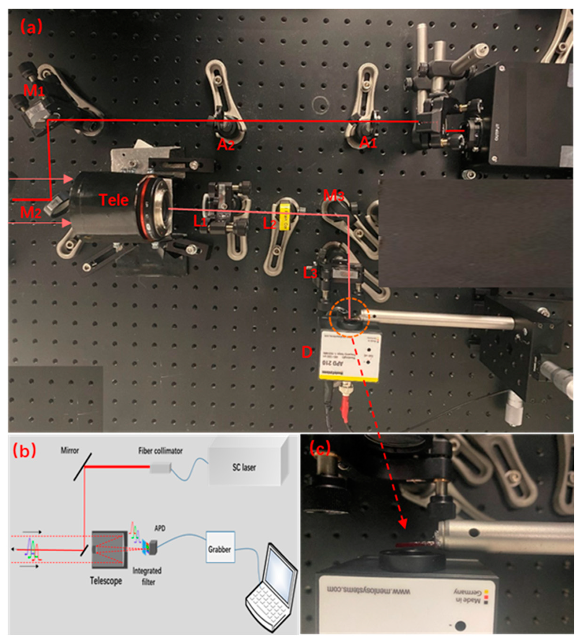
2.2. System Configuration

The schematic of the 6-channel IOF-HSL model is shown in Figure 2. An SC laser (YSL© OEM) spreading over a 400 to 2400 nm laser beam was employed as the laser source. The SC laser’s pulse width (full width at half maximum, FWHM) was 10 nanoseconds (ns) at a repetition rate of 0.01–1 kHz. The laser beam was collimated with a fiber collimator and then pointed to targets by two steering mirrors (M1, M2); the apertures (A1, A2) here were used to calibrate the optical circuit. A Cass-grain telescope (Tele, Samyang 300 mm F/6.3) was used to collect primary echoes from targets. Here, in the optics, two lenses (L1, L2) were used as a collimator and then to focus by the third lens (L3). The IOF was installed in the aft optics of this HSL system by a fretting platform, and clinging to the APD sensors (D). The passband can be chosen by modulating the fretting platform in the X direction. The echoes were split into 6 channels by the IOF and then focused on a Si-APD sensor (Thorlab-APD 210, 400–1100 nm). We chose an APD covering the 400–1000 nm wavelength range; its maximum gain was 2.5 × 10⁵ V/W @800 nm and maximum photosensitivity can achieve 50 A/W @800 nm. Through moving the IOF step by step to couple with a single-element APD sensor, 6-channel information can be collected by this Si-APD sensor. In this HSL prototype, a high-speed digitizer card (10 GS/s) was used to record the analogue signals from the Si-APD. With such a system schematic setting, the characterizations of the IOF-HSL prototype can be preliminary verified.

2.3. Experiments System

Several experiments were used to test the performance of the IOF-HSL prototype. More details are shown in Table 2. All the experiments were conducted in a light-controlled environment to obtain a high signal/noise ratio (SNR) result. Firstly, through measurement of the echo from the targets (standard reflective boards from SVC© with 60% (SRB-60%)) placed at different locations, we calibrated the IOF-HSL prototype. Here, the echo waveforms from an SRB-99% were also measured as the reflectance. Then, the ranging performance of the IOF-HSL prototype was carried out by testing the ranging accuracy of different targets at different distances. In addition, several kinds of targets (placed at a distance of 8.0 m from the HSL) with different spectral characteristics were employed to test their performance in spectral profiles. The oranges and carrots with similar appearance were measured to test the IOT-HSL’s capability in the material distinction. The spectral profiles from green/dry leaves and 3 kinds of dry pine wood were collected to test its capability to monitor the plant’s health status and water content. Three typical ores’ samples (quartz, plagioclase, and talc) were measured to test the IOF-HSL use for ore classification, which is widely used in mining.

3. Typographical Style

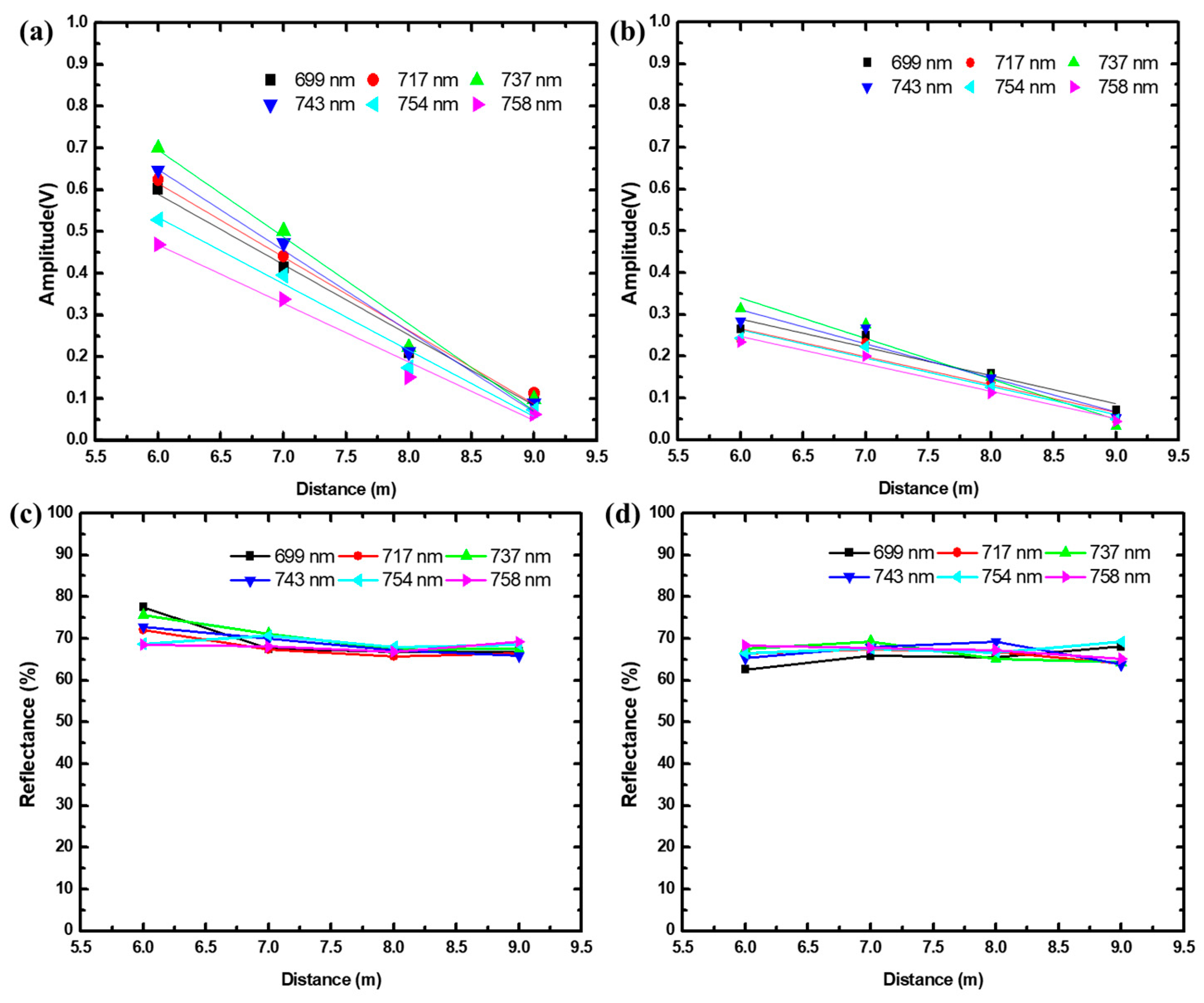
3.1. System Calibration
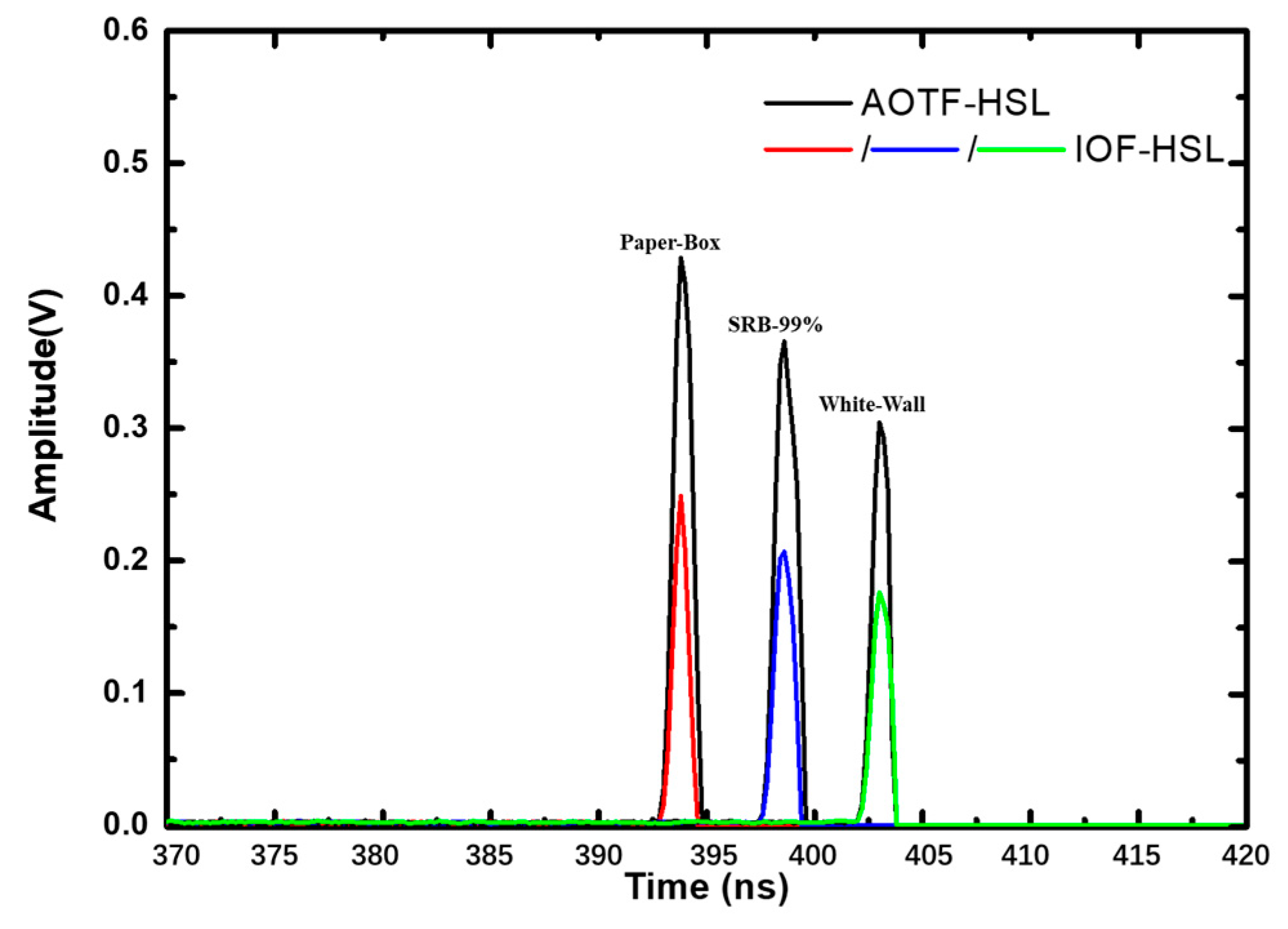
The echo waveforms from an identical SRB-60% (at distances of 6 m, 7 m, 8 m, and 9 m) were collected by the IOF-HSL prototype and AOTF-HSL simultaneously. All the data given here were the average values obtained by eight data samples. Figure 3a,b show that the echo intensity at each channel collected by the IOF all decreased as the distances increased from 6 m to 9 m, and the fitting results also showed a more linear relationship, which was followed by the Lidar Equation [3]:
P r = α × P t 4 π R 2
where Pr is the echo power received, Pt is the laser source power, R is the distance, and α is the parameter determined by the system and experiment (such as laser beam width, receiver optics, and surface reflectance and receiving area of the scatter). Compared with the AOTF-HSL, the echo intensity collected by the IOF-HSL was a little lower due to the transamination of the IOF components. After calibration by the SRB-99%, we obtained the reflectance of the IOF-HSL, shown in Figure 3c,d, which was an important factor that was used for target classification. In Figure 3c,d, we can see that the IOF-HSL’s capability in reflectance was almost uninfluenced by the lower transamination of the IOF components. Therefore, the IOF component shows the same effectiveness spectroscopically in the HSL system as other complex spectroscopic devices (such as AOTF and LCTF).

3.2. Ranging

The ranging capability of the designed IOF-HSL prototype can be evaluated by a distance test and could also further demonstrate its essential hyperspectral detection capability. Here, we chose the waveforms of one measurement (@758 nm) during the laboratory test collected by the high-speed digitizer card as shown in Figure 4. In this test, a paper box (white), SRB-99%, and white wall were used as the measured targets, which were placed at distances of 7.8 m, 8.5 m, and 9.2 m from the laser source, respectively, to test the IOF-HSL’s ranging capability. The AOTF-HSL also employed measurement as a comparison; the results are labelled as black lines.
In our system, the trigger signal was utilized as the start point of the time-of-flight measurement in the laser source. The peak positions of the three curves in Figure 4 are 393.8 ns, 398.6 ns, and 403.0 ns, respectively, which implies that the exact distances of the paper box, SRB-99%, and white wall were 7.82 m, 8.54 m, and 9.20 m from the laser source. The result verified that the IOF-HSL achieved a ranging accuracy as high as 0.01 m. Compared with the AOTF-HSL, the intensity of the ringing waveform collected by the IOF-HSL was lower, but the ranging accuracy was strictly coincident. In addition, although the reference range is infeasible to determine under current optics system settings, we can rectify the system error and improve the accuracy of the range measurements through the post-calibration procession.

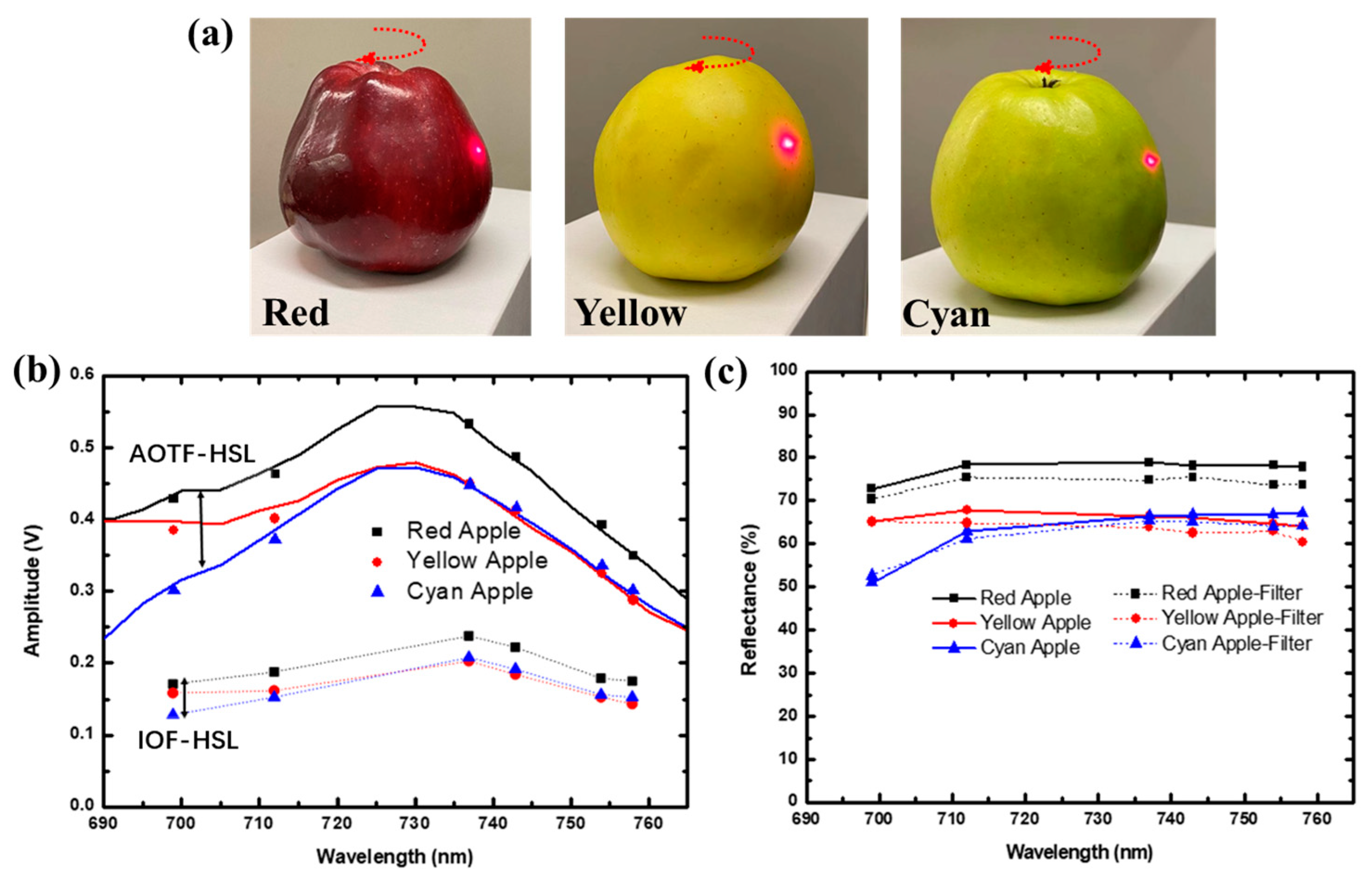
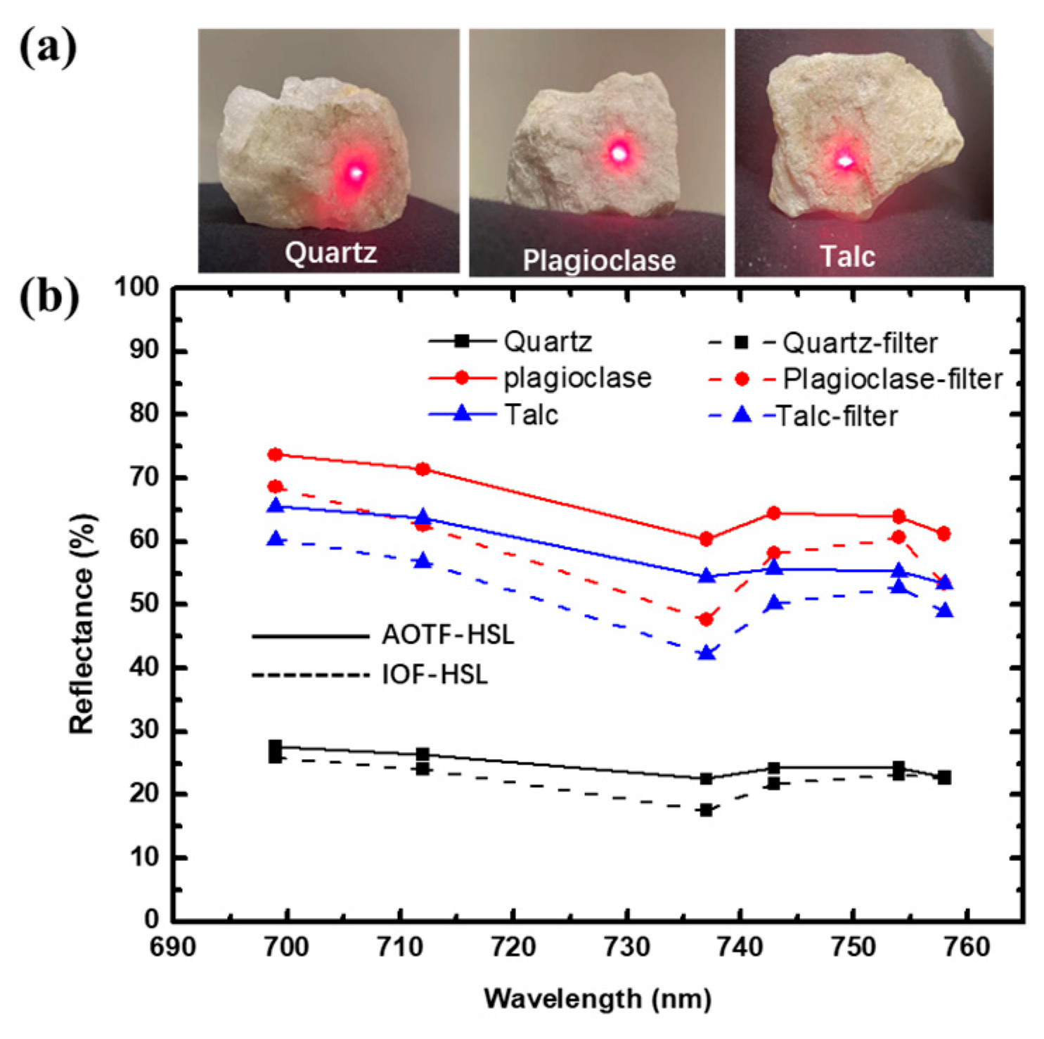
3.3. Spectral Profiles

Because the IOF’s channels mainly covered the wave band of 690–760 nm, we chose targets that appear orange-yellow in appearance to measure spectral profiles first. An orange and carrot were chosen as the typically measured targets, and an AOTF-HSL was also employed to test as a reference. By adjusting (rotating or translating) the targets in the direction shown in Figure 5a, we collected eight series of data in different surface areas and gave the average values. Figure 5b shows that the echo waveforms collected by the IOF-HSL were slightly lower than those of the AOTF-HSL; the reason should be attributed to the condition of the IOF component installed, whereas the reflectance obtained by the AOTF-HSL and IOF-HSL prototype coincided well for the same targets. Compared with the carrot, the orange shows a higher reflectance at all six channels (Figure 5b). The higher reflectance of the orange was attributed to the smoother surface of the orange and the content of water, sugar, and other components. The spectra and variation of the orange and carrot collected by both the AOTF-HSL and IOF-HSL were similar (Figure 5), which implies that the two targets exhibit similar appearances. These preliminary spectral profile results verified that the IOF could be employed as the key spectroscopic component in the HSL prototype.
Furthermore, the spectral profiles from apples that appear as red, yellow, and cyan were used to test the IOF-HSL’s capability in distinguishing targets’ appearance. All of the three apples were cleaned with water at 50 °C for 5 min to remove the wax layer on the surface. By rotating these apples, in the direction shown in Figure 6a, we collected eight series of data in different surface areas and gave the average values. The transamination of the IOF components slightly declined the amplitude intensity of echoes collected by the IOF-HSL, but the spectral profile was in accordance with that of the AOTF-HSL (Figure 6b). The reflectance of the red apple was slightly higher than the other two apples, which should be attributed to the red apple being wrapped with a thick and smoother peel. The red spectral appearance also induced a relatively higher reflectance, especially for the channel at 699 nm. The cyan spectral appearance induced a much lower reflectance [19]. The spectral profiles of the three spectra collected by the IOF-HSL prototype verified their applications in appearance classification.
The primary spectral profiles result from the two sets of objects, which appear as the same color consisting of different materials (components, sugar, etc.) and consist of the same materials appearing as a different color, verifying the capability of the IOF-HSL prototype to distinguish color and materials. This verification can be used in agricultural product classification and screening, including fruits, vegetables, and many other products. For large-scale classification, such as trees, crops, and forests, the IOF-HSL prototype will show much more attractive applications. Therefore, further research on spectral classification based on the IOF-HSL prototype covering a wider passband range will be carried out in our later reports.
The appearance, water concentrations, and surface characteristics of targets induced different spectral profiles, which have been widely used in forestry and agriculture classification. The IOF-HSL prototype was verified effectively in the spectral profile collecting based on the vegetables and fruits. Here, the spectral profiles of green/dry leaves and three kinds of dry wood (Figure 7a) were measured by the IOF-HSL prototype to test its capability in forest classification, and further compared with the NDVI (a typical parameter in forestry) of the target to perform its applications in classification. In Figure 7b, the higher intensity of the echo waveforms from the dry wood was induced by the smoother surface layer, and such a phenomenon can be obtained by both AOTF-HSL and IOF-HSL prototypes.
The echo’s highest waveforms from the green leaf, which also shows a smoother surface layer, are at around 737 nm. The smoother surface layer effective in the spectral profiles can be further verified by comparing the reflectance and waveform intensity from the dry wood inside and outside. The dry wood and wood with moss can be distinguished by the spectral profiles in the shorter wavelength bands (699 and 712 nm). In addition, the dry leaf shows a lower reflectance than the green leaf and the other two kinds of wood. The lower reflectance was attributed to the smoother surface layer, and the different spectral profiles should be attributed to the chlorophyll in green leaves, including the leaf pigment content and the leaf structure, inducing higher reflectance spectrums [20,21]. Generally, green plants usually exhibit higher reflectance in the red-edge and near-infrared (NIR) band, and chlorophyll exhibits a higher absorption in the red band [3,22,23,24]. Therefore, the reflectance of the green leaf increased as the wavelength increased from 699 nm to 758 nm, which was largely different from the dry leaf and wood (Figure 7c).
Additionally, the NDVI parameters of these leaves and wood were also obtained from the reflectance spectral profiles, shown in Figure 7d. The green leaf showed a much higher NDVI than the dry leaf and wood, which further verified that the chlorophyll affects the spectral profiles. The moss on the wood’s surface layer also influenced the NDVI parameters, leading to a large difference in NDVI between the dry leaf and wood. The dry wood without moss (both the outside and inside surface) showed lower NDVI parameters. The increase in NDVI induced by the moss further verifies the accuracy of the spectral profile collected by the IOF-HSL prototype. The spectral profile and corresponding NDVI parameters based on the IOF-HSL prototype exhibit its performance in vegetation classification.
The spectra profiles from ore samples (quartz, plagioclase, and talc) were measured to explore the IOF-HSL’s capabilities in geological material detection and classification. Among the three kinds of ores shown in Figure 8a, it was difficult to distinguish them in appearance due to almost the same appearance and materials, whereas Figure 8b shows that the talc has a much lower reflectance than that of quartz and plagioclase at all six channels, making it easier to distinguish the talc from quartz and plagioclase. And the reflectance between quartz and plagioclase was also different (about 10%), which can help us to distinguish these two ores. Furthermore, the spectral variation of the talc was also different from the other two ores, especially in the range of longer than 737 nm. This should be attributed to the different composition and internal structures. Based on the spectral variation, we can distinguish that the talc was composed of different materials from quartz and plagioclase. Therefore, the spectra profiles from ore samples make the IOF-HSL show potential applications in geological detection and classification.
Generally, the ranging and spectral profile results based on the IOF can arrive at the AOTF and any other spectroscopic devices, which are composed of complex and bulky structures. However, the IOF employed here shows a comparatively lower transmittance and only six channels compared to bulky components with lower integration. These results further verify that the IOF component can, instead of the complex and bulky spectroscopic devices, promote the miniaturizing of the HSL system. The further integrated scheme of the IOF and the detector will be given in our further research.

3.4. Coupling IOF and Sensor

Traditionally, the HSL could employ single-element APD to collect the echo signal, shown in Figure 9a, and could not obtain information at different spectral channels simultaneously, which also degraded the flexibility and integration of the system. The dominant reason was attributed to that the spectroscopic devices employed in the HSL system could not match well with the sensors. The IOF component could integrate well with APD array sensors. Here, we moved the IOF step by step to couple with a single-element APD sensor (Figure 9b) and preliminarily verified its capability to collect six-channel information simultaneously. This method has been used to verify the ranging and spectral profile capability of the IOF-HSL. Furthermore, based on the array detector, the IOF component could include a tight couple with the sensor through the strip and 2-dimension distributions, shown in Figure 9c,d, which will further the miniaturization of the HSL system. As an attempt, based on an array IOF, a chip-spectrometer covering 900–1700 nm with a spectral resolution of 2 nm has been reported [17]. This chip-spectrometer paved the way for further miniaturizing the IOF-HSL and also made the IOF-HSL much more integrated and functionalized. A miniature IOF-HSL customized to work in the VIS or IR band for target classification and distinguishing will further promote the IOF-HSL’s wide applications in autopilot, artificial intelligence, and many other fields.

4. Conclusions

In conclusion, a six-channel IOF-HSL prototype was proposed, and its performance in ranging and spectral profile collecting was preliminarily tested. The location of paper box, SRB-99%, and white wall measurement by the IOF-HSL illustrated that its ranging accuracy was the same as that of the AOTF-HSL. The ranging capability promotes that the IOF-HSL could mend the need for the three-dimensional reconstruction of targets. Then, the spectral profiles of the orange and carrot tested the IOF-HSL’s capability in distinguishing appearance, and three apples (appearing as red/yellow/cyan) further verified its capability in appearance classification. These spectral profiles verified that the IOF-HSL will show optional application in the distinguishing of fruits and vegetables. The spectral profiles of green/dry leaves and different wood, combined with the NDVI parameters, illustrated that the IOF-HSL was effectively applied to forestry classification. The miniature HSL system could especially have applications in unmanned aerial vehicles (UAVs), handheld platforms optional for a forest and agriculture. The spectral profiles of ores with similar surface layers and appearance further verified the IOF-HSL’s illustrated applications in geological material detection and classification, which will also promote the HSL system’s use in deep space detection and asteroid exploration. Although the transmittance of the IOF used here was a little lower, which mitigated the amplitude of the echo waveforms, it almost did not influence the IOF-HSL’s performance in classification. Additionally, based on the conception of integration, an array IOF integrated with an array detector will be further manufactured to improve the miniaturization of the HSL and also make the IOF-HSL much more flexible. The miniaturizing and integration of the IOF-HSL system will show wider applications in auto-drive, artificial intelligence, and many other fields.

Author Contributions

Conceptualization, Y.C., Z.S., and H.S.; methodology, Y.C., S.S., X.Y., and H.S.; software, Y.W. and J.J.; formal analysis, H.S. and S.W.; resources, Y.C.; data curation, C.J. and P.H.; writing—original draft preparation, H.S.; writing—review and editing, Y.C. and H.S.; visualization, H.Y.; supervision, Y.C., M.K., and J.H.; project administration, Y.C. and S.S. All authors have read and agreed to the published version of the manuscript.

Funding

Academy of Finland (No. 336145, No. 349229), Open Funding of the State Key Laboratory of Pulsed Power Laser Technology (No. SKL2023KF40), Shanghai Pu Jiang Program (No. 23PJ1414800) and Scientific Research Projects of National University of Defense Technology (No. 22-ZZCX-07).

Data Availability Statement

The data presented in this study are available on request from the corresponding author due to privacy restrictions.

Conflicts of Interest

The authors declare no conflicts of interest.

References

  1. Kaasalainen, S.; Lindroos, T.; Hyyppa, J. Toward Hyperspectral Lidar: Measurement of Spectral Backscatter Intensity With a Supercontinuum Laser Source. IEEE Geosci. Remote Sens. Lett. 2007, 4, 211–215. [Google Scholar] [CrossRef]
  2. Sun, J.; Shi, S.; Gong, W.; Yang, J.; Du, L.; Song, S.; Chen, B.; Zhang, Z. Evaluation of hyperspectral LiDAR for monitoring rice leaf nitrogen by comparison with multispectral LiDAR and passive spectrometer. Sci. Rep. 2017, 7, 40362. [Google Scholar] [CrossRef]
  3. Ghamisi, P.; Rasti, B.; Yokoya, N.; Wang, Q.M.; Hofle, B.; Bruzzone, L.; Bovolo, F.; Chi, M.M.; Anders, K.; Gloaguen, R.; et al. Multisource and multitemporal data fusion in remote sensing a comprehensive review of the state of the art. IEEE Geosci. Remote Sens. Mag. 2019, 7, 6–39. [Google Scholar] [CrossRef]
  4. Huo, L.-Z.; Silva, C.A.; Klauberg, C.; Mohan, M.; Zhao, L.-J.; Tang, P.; Hudak, A.T. Supervised spatial classification of multispectral LiDAR data in urban areas. PLoS ONE 2018, 13, e0206185. [Google Scholar] [CrossRef] [PubMed]
  5. Fernandez Diaz, J.; Carter, W.; Glennie, C.; Shrestha, R.; Pan, Z.; Ekhtari, N.; Singhania, A.; Hauser, D.; Sartori, M. Capability Assessment and Performance Metrics for the Titan Multispectral Mapping Lidar. Remote Sens. 2016, 8, 936. [Google Scholar] [CrossRef]
  6. Wallace, A.M.; McCarthy, A.; Nichol, C.J.; Ren, X.M.; Morak, S.; Martinez-Ramirez, D.; Woodhouse, I.H.; Buller, G.S. Design and Evaluation of Multispectral LiDAR for the Recovery of Arboreal Parameters. IEEE Trans. Geosci. Remote Sens. 2013, 52, 4942–4954. [Google Scholar] [CrossRef]
  7. Song, S.; Wang, B.; Gong, W.; Chen, Z.; Lin, X.; Sun, J.; Shi, S. A new waveform decomposition method for multispectral LiDAR. ISPRS J. Photogramm. Remote Sens. 2019, 149, 40–49. [Google Scholar] [CrossRef]
  8. Liu, H.; Yu, T.; Hu, B.; Hou, X.; Zhang, Z.; Liu, X.; Liu, J.; Wang, X.; Zhong, J.; Tan, Z.; et al. UAV-Borne Hyperspectral Imaging Remote Sensing System Based on Acousto-Optic Tunable Filter for Water Quality Monitoring. Remote Sens. 2021, 13, 4069. [Google Scholar] [CrossRef]
  9. Aruffo, E.; Chiuri, A.; Angelini, F.; Artuso, F.; Cataldi, D.; Colao, F.; Fiorani, L.; Menicucci, I.; Nuvoli, M.; Pistilli, M.; et al. Hyperspectral Fluorescence LIDAR Based on a Liquid Crystal Tunable Filter for Marine Environment Monitoring. Sensors 2020, 20, 410. [Google Scholar] [CrossRef]
  10. Hegyi, A.; Martini, J. Hyperspectral imaging with a liquid crystal polarization interferometer. Opt. Express 2015, 23, 28742–28754. [Google Scholar] [CrossRef]
  11. Du, L.; Gong, W.; Shi, S.; Yang, J.; Sun, J.; Zhu, B.; Song, S. Estimation of rice leaf nitrogen contents based on hyperspectral LIDAR. Int. J. Appl. Earth Obs. Geoinf. 2016, 44, 136–142. [Google Scholar] [CrossRef]
  12. Sun, H.; Wang, Z.; Chen, Y.; Tian, W.; He, W.; Wu, H.; Zhang, H.; Tang, L.; Jiang, C.; Jia, J.; et al. Preliminary verification of hyperspectral LiDAR covering VIS-NIR-SWIR used for objects classification. Eur. J. Remote Sens. 2022, 55, 291–303. [Google Scholar] [CrossRef]
  13. Devgan, P.S.; Pruessner, M.W.; Urick, V.J.; Williams, K.J. Detecting Low-Power RF Signals Using a Multimode Optoelectronic Oscillator and Integrated Optical Filter. IEEE Photon Techl. 2009, 22, 152–154. [Google Scholar] [CrossRef]
  14. D’Alessandro, A.; Donisi, D.; De Sio, L.; Beccherelli, R.; Asquini, R.; Caputo, R.; Umeton, C. Tunable integrated optical filter made of a glass ion-exchanged waveguide and an electro-optic composite holographic grating. Opt. Express 2008, 16, 9254–9260. [Google Scholar] [CrossRef]
  15. Wang, S.-W.; Chen, X.; Lu, W.; Wang, L.; Wu, Y.; Wang, Z. Integrated optical filter arrays fabricated by using the combinatorial etching technique. Opt. Lett. 2006, 31, 332–334. [Google Scholar] [CrossRef] [PubMed]
  16. Agrawal, P.; Tack, K.; Geelen, B.; Masschelein, B.; Moran, P.M.A.; Lambrechts, A.; Jayapala, M. Characterization of VNIR Hyperspectral Sensors with Monolithically Integrated Optical Filters. Electron. Imaging 2016, 28, 1–7. [Google Scholar] [CrossRef]
  17. Mao, C.-X.; Gao, S.; Wang, Y.; Wang, Z.; Qin, F.; Sanz-Izquierdo, B.; Chu, Q.-X. An Integrated Filtering Antenna Array With High Selectivity and Harmonics Suppression. IEEE Trans. Microw. Theory Tech. 2016, 64, 1798–1805. [Google Scholar] [CrossRef]
  18. Wang, S.-W.; Li, M.; Xia, C.-S.; Wang, H.-Q.; Chen, X.-S.; Lu, W. 128 channels of integrated filter array rapidly fabricated by using the combinatorial deposition technique. Appl. Phys. B 2007, 88, 281–284. [Google Scholar] [CrossRef]
  19. Xuan, Z.; Wang, Z.; Liu, Q.; Huang, S.; Yang, B.; Yang, L.; Yin, Z.; Xie, M.; Li, C.; Yu, J.; et al. Short-Wave Infrared Chip-Spectrometer by Using Laser Direct-Writing Grayscale Lithography. Adv. Opt. Mater. 2022, 10.19, 2200284. [Google Scholar] [CrossRef]
  20. Escobar, D.E.; Everitt, J.H.; Davis, M.R.; Fletcher, R.S.; Yang, C. Relationship between Plant Spectral Reflectances and their Image Tonal Responses on Aerial Photographs. Geocarto Int. 2002, 17, 65–76. [Google Scholar] [CrossRef]
  21. Main, R.; Cho, M.A.; Mathieu, R.; O’Kennedy, M.M.; Ramoelo, A.; Koch, S. An investigation into robust spectral indices for leaf chlorophyll estimation. ISPRS J. Photogramm. Remote Sens. 2011, 66, 751–761. [Google Scholar] [CrossRef]
  22. Hakala, T.; Suomalainen, J.; Kaasalainen, S.; Chen, Y. Full waveform hyperspectral LiDAR for terrestrial laser scanning. Opt. Express 2012, 20, 7119–7127. [Google Scholar] [CrossRef] [PubMed]
  23. Buschmann, C.; Lenk, S.; Lichtenthaler, H.K. Reflectance spectra and images of green leaves with different tissue structure and chlorophyll content. Isr. J. Plant Sci. 2012, 60, 49–64. [Google Scholar] [CrossRef]
  24. Xie, Q.; Dash, J.; Huang, W.; Peng, D.; Qin, Q.; Mortimer, H.; Casa, R.; Pignatti, S.; Laneve, G.; Pascucci, S.; et al. Vegetation Indices Combining the Red and Red-Edge Spectral Information for Leaf Area Index Retrieval. IEEE J. Sel. Top. Appl. Earth Obs. Remote Sens. 2018, 11, 1482–1493. [Google Scholar] [CrossRef]
Figure 1. (ae) A diagram of the procedure for fabricating the IOF filter; (f) the IOF component compared with a coin.
Remotesensing 16 01642 g001
Figure 2. (a) The optical schematic and (b) system setup of the 6-channel IOF-HSL; (c) shows the details of the structure of the IOF and the APD detector.
Remotesensing 16 01642 g002
Figure 3. The echo waveforms from an SRB-60% collected by the (a) AOTF-HSL and (b) IOF-HSL at distances of 6 m, 7 m, 8 m, and 9 m; (c,d) are the corresponding reflectance calibrated by an SRB-99%. The straight line in (a,b) is the linear fitting result.
Remotesensing 16 01642 g003
Figure 4. The waveforms from a paper box, SRB-99%, and white wall at different distances.
Remotesensing 16 01642 g004
Figure 5. (a) An orange and carrot, the arrows are the rotating direction; (b) the echo waveforms and (c) reflectance of each spectral channel, and the solid lines in (b,c) are the spectral profiles obtained by the AOTF-HSL.
Remotesensing 16 01642 g005
Figure 6. (a) three apples with different appearances, the arrows are the rotating direction; (b) the echo waveform and (c) the reflectance of each spectral channel.
Remotesensing 16 01642 g006
Figure 7. (a) Green/dry leaves and three kinds of dry wood, (b) the waveforms and (c) reflectance of each target, and (d) the Normalized Difference Vegetation Index (NDVI) parameters based on spectral profiles are also given.
Remotesensing 16 01642 g007
Figure 8. (a) three kinds of ores irradiated with the laser and (b) the corresponding spectral profiles collected by the IOF-HSL prototype.
Remotesensing 16 01642 g008
Figure 9. (a) HSL based on single-element APD, and IOF-HSL prototype employing (b) single-element APD with strip IOF; (c) array detector with strip IOF; and (d) array detector with array IOF.
Remotesensing 16 01642 g009
Table 1. The central wavelength and the bandwidth of the IOF.
λ (nm)699712737743754758
Δλ (nm)54.54.54.54.55
T (%)43%40%46%48%48%54%
Table 2. Experiment setting.
ExperimentTest ProposedTargets
1System CalibrationSignals from each channel
Signals from different distances
SRB-60%, SRB-99%
2Ranging Testing the ranging accuracy based on IOFSRB-99%, White Wall, Paper Box
3Spectral ProfilesDistinguish targets’ appearance and materialsOrange, Carrots, Red/Yellow/Cyan Apple
Monitoring the plantsGreen/Dry Leaf, 3 Kinds of Dry Pine Wood
Analysis of ore speciesQuartz, Plagioclase, Talc
Disclaimer/Publisher’s Note: The statements, opinions and data contained in all publications are solely those of the individual author(s) and contributor(s) and not of MDPI and/or the editor(s). MDPI and/or the editor(s) disclaim responsibility for any injury to people or property resulting from any ideas, methods, instructions or products referred to in the content.

