
An Advanced Quality Assessment and Monitoring of ESA Sentinel-1 SAR Products via the CyCLOPS Infrastructure in the Southeastern Mediterranean Region
 ,
,
Abstract
:1. Introduction
2. Theoretical Background
2.1. Radar Backscatter Coefficient
2.2. Radar Brightness
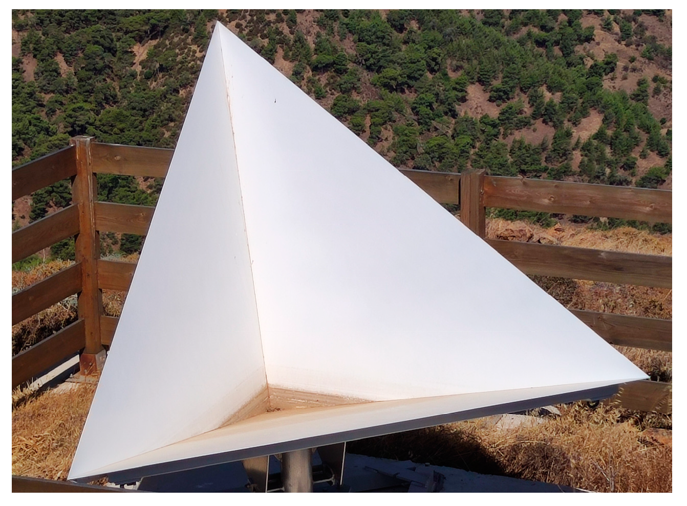
2.3. SAR Corner Reflectors
2.4. SAR Calibration Using Point Target Analysis
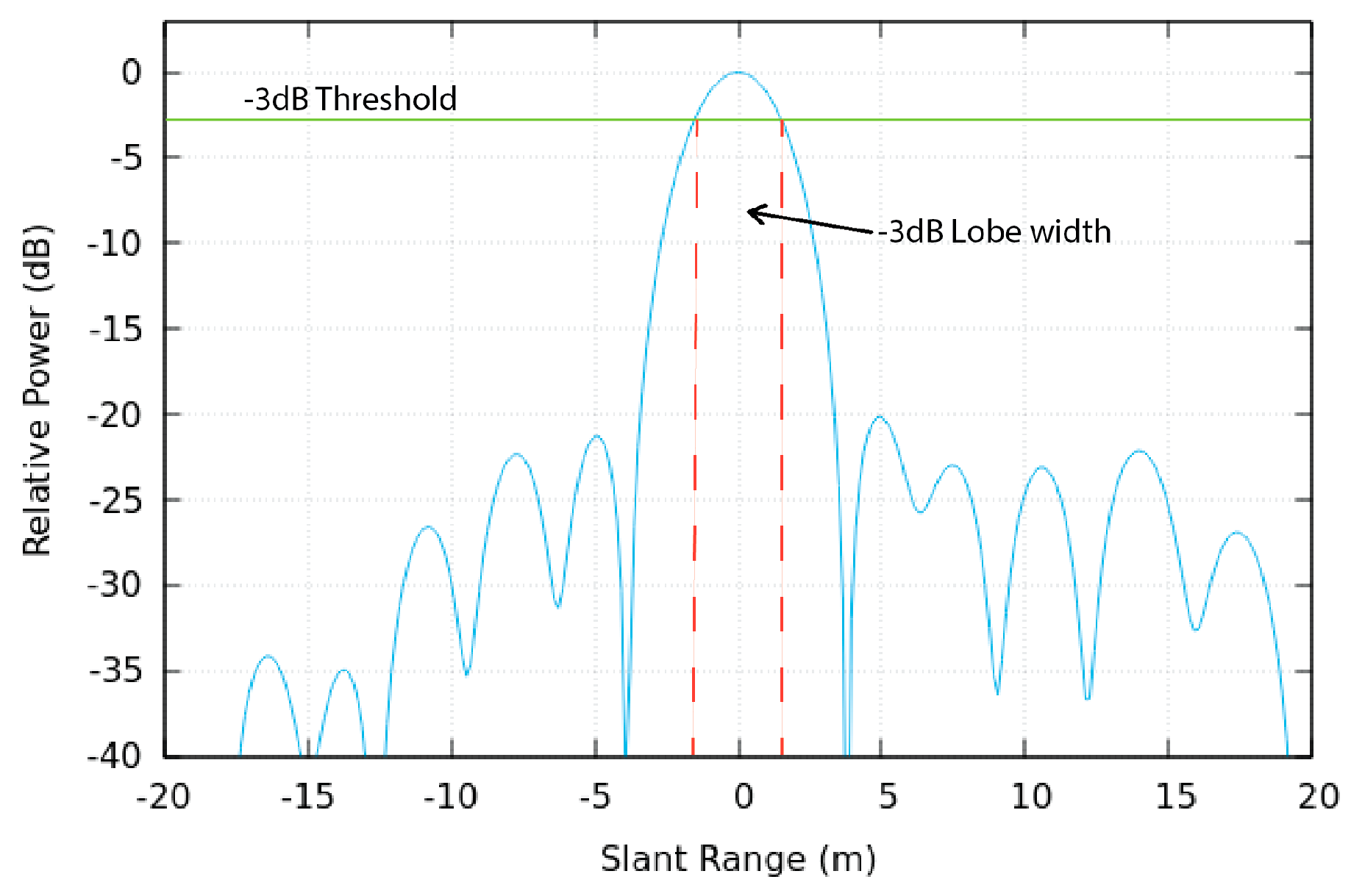
2.4.1. Impulse Response Function
- Spatial Resolution in SAR imaging
- 2.
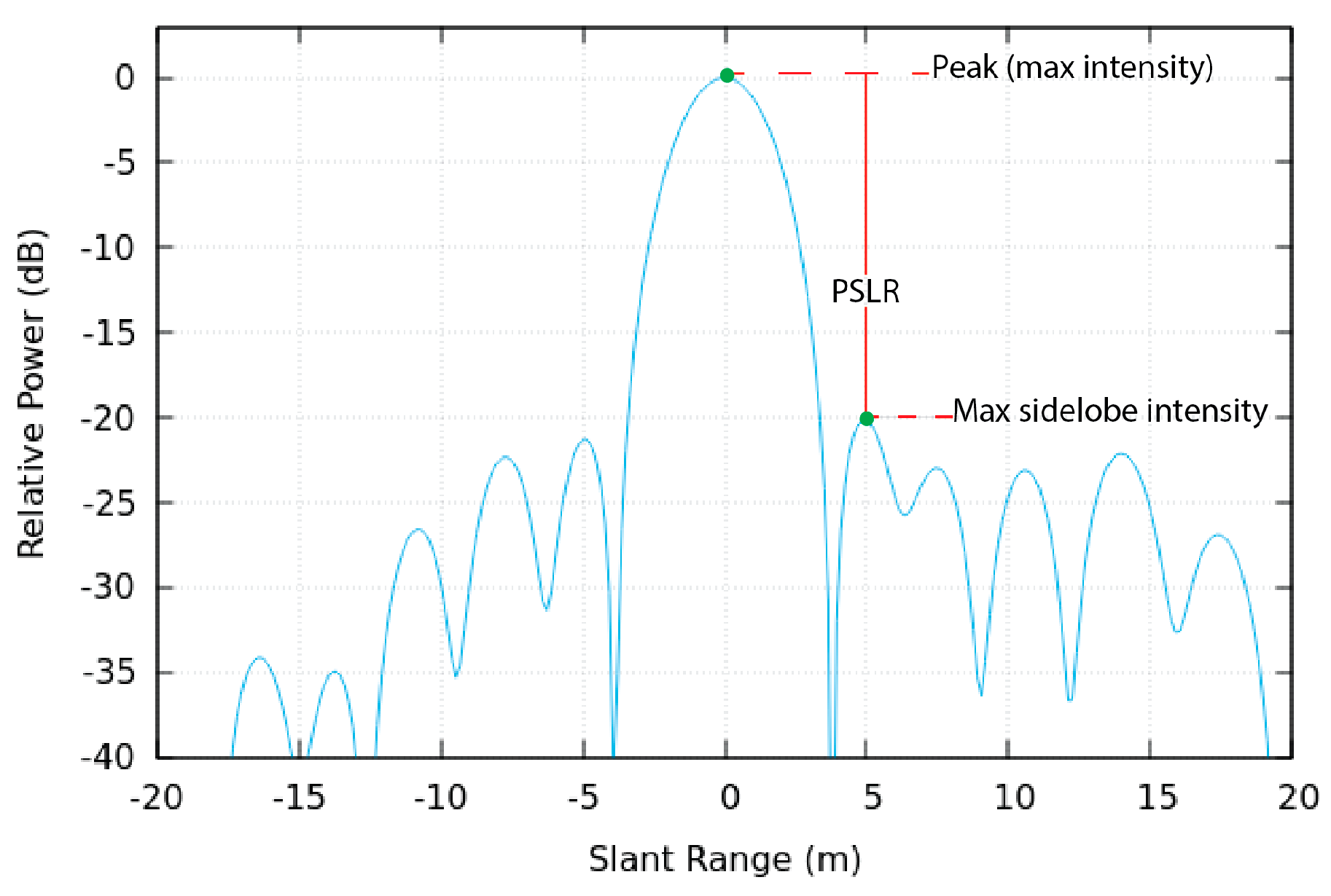
- Sidelobe Level
2.4.2. Radar Cross-Section
2.4.3. Signal-to-Clutter Ratio
2.4.4. Slant Distance Error in LoS
2.4.5. Geolocation Analysis
- 3.
- Oversampling the SLC image to accurately estimate the position of the target, which is expressed in range and azimuth time coordinates; thus, the estimated pixel coordinates of the TTCR are transformed into time coordinates.
- 4.
- Inverse geocoding to extract the azimuth time at which the satellite obtains the image with the CR’s position.
- 5.
- The final step entails the estimation of the location error in the radar time coordinate system which is defined as the difference between the measured position and the expected coordinates of the CR. These time differences can then be transformed into units of length, defining the ALE, following the process explained in [53].
3. Performance Assessment of TTCRs
3.1. Image Quality Performance
- 6.
- Spatial Resolution
- 7.
- Sidelobe Level
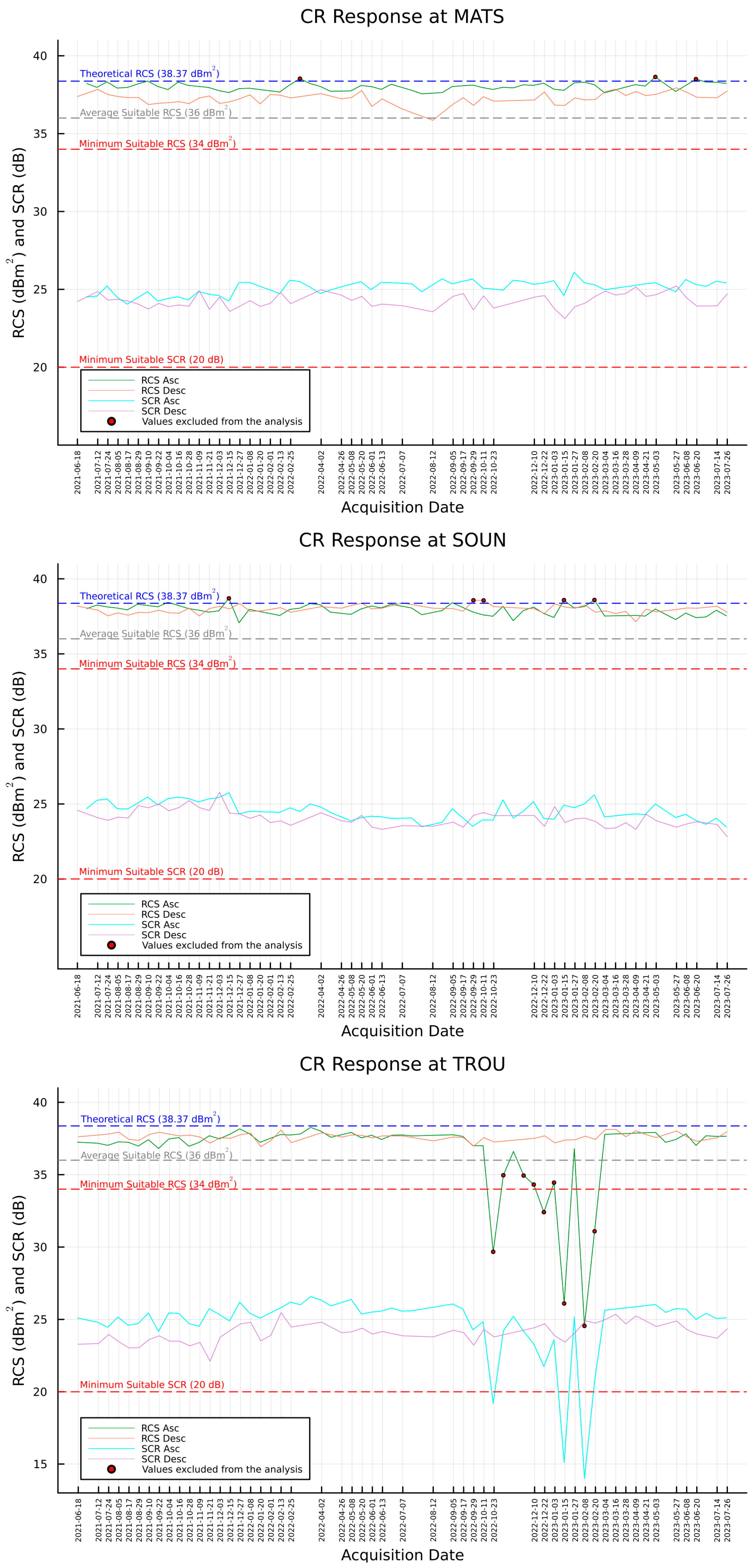
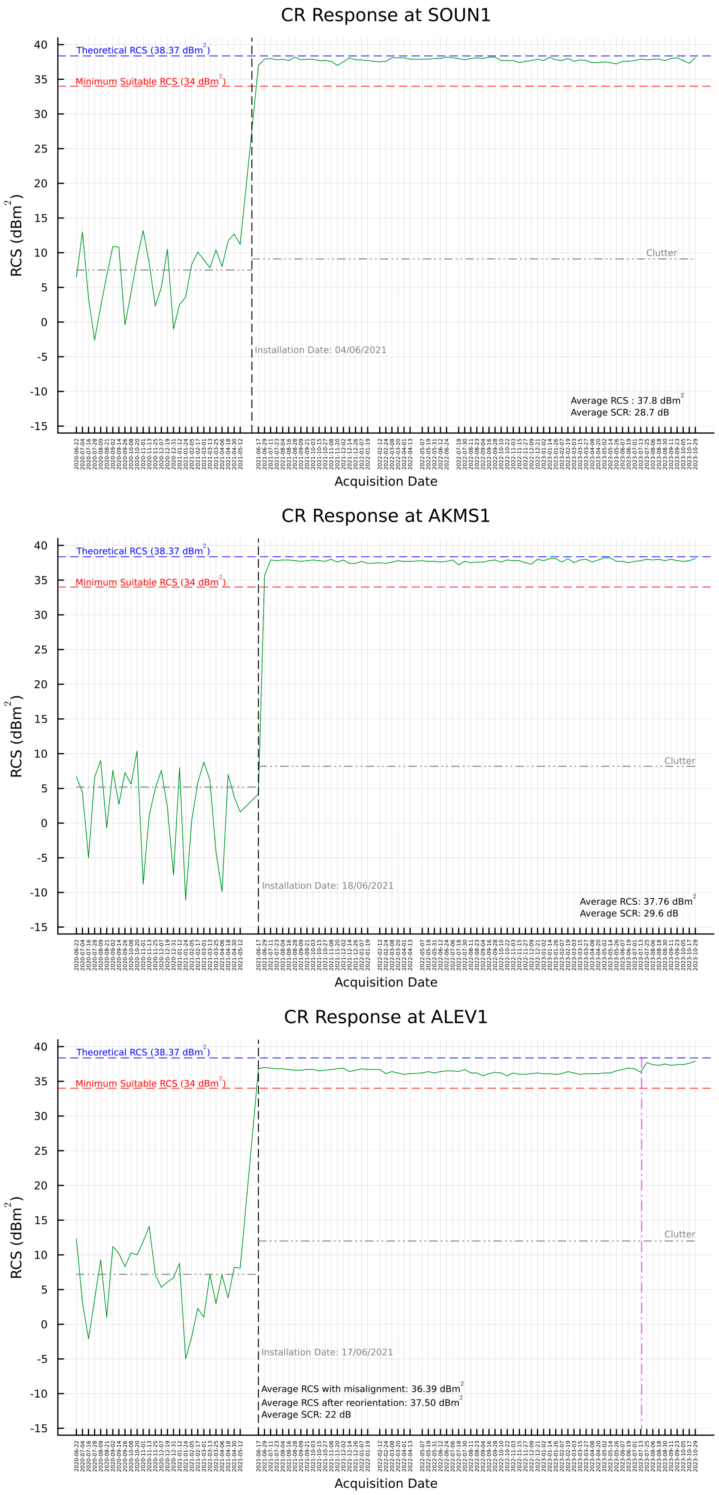
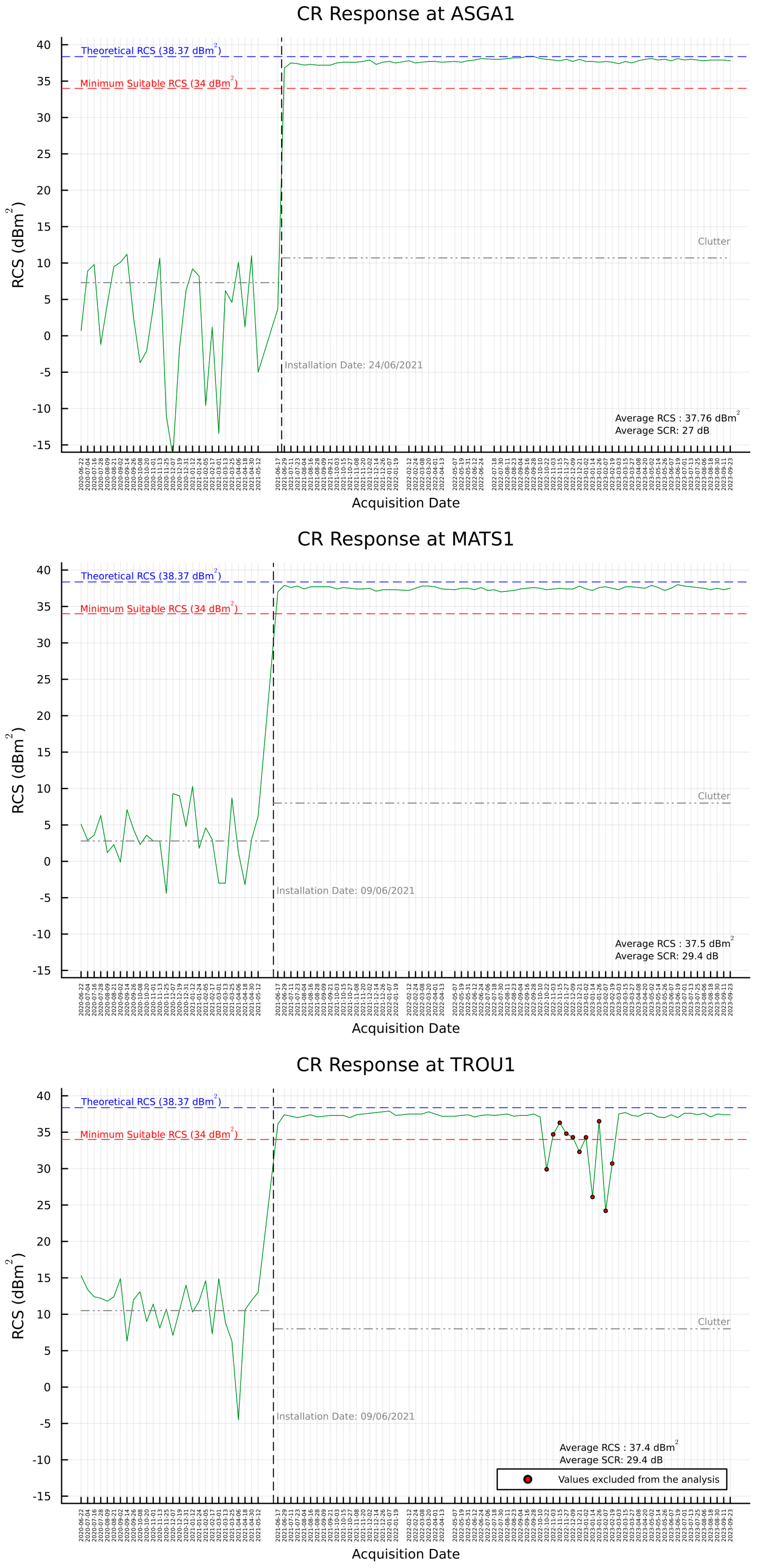
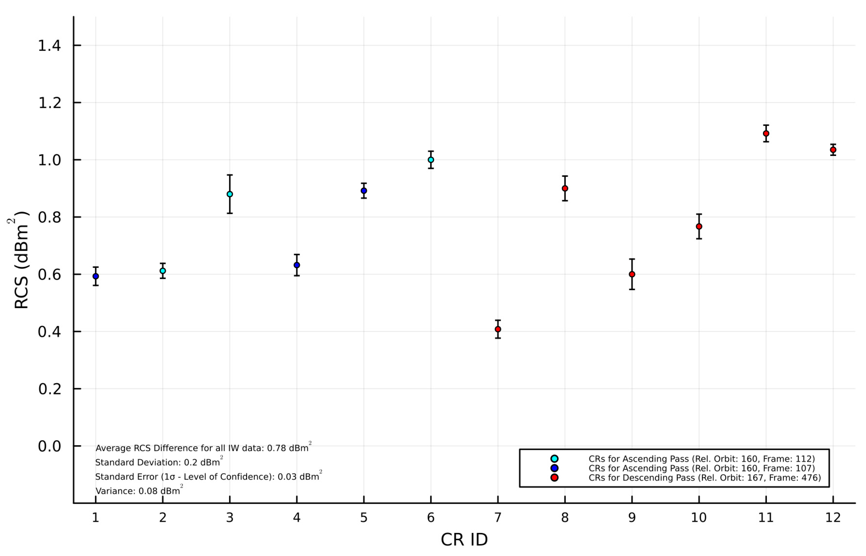
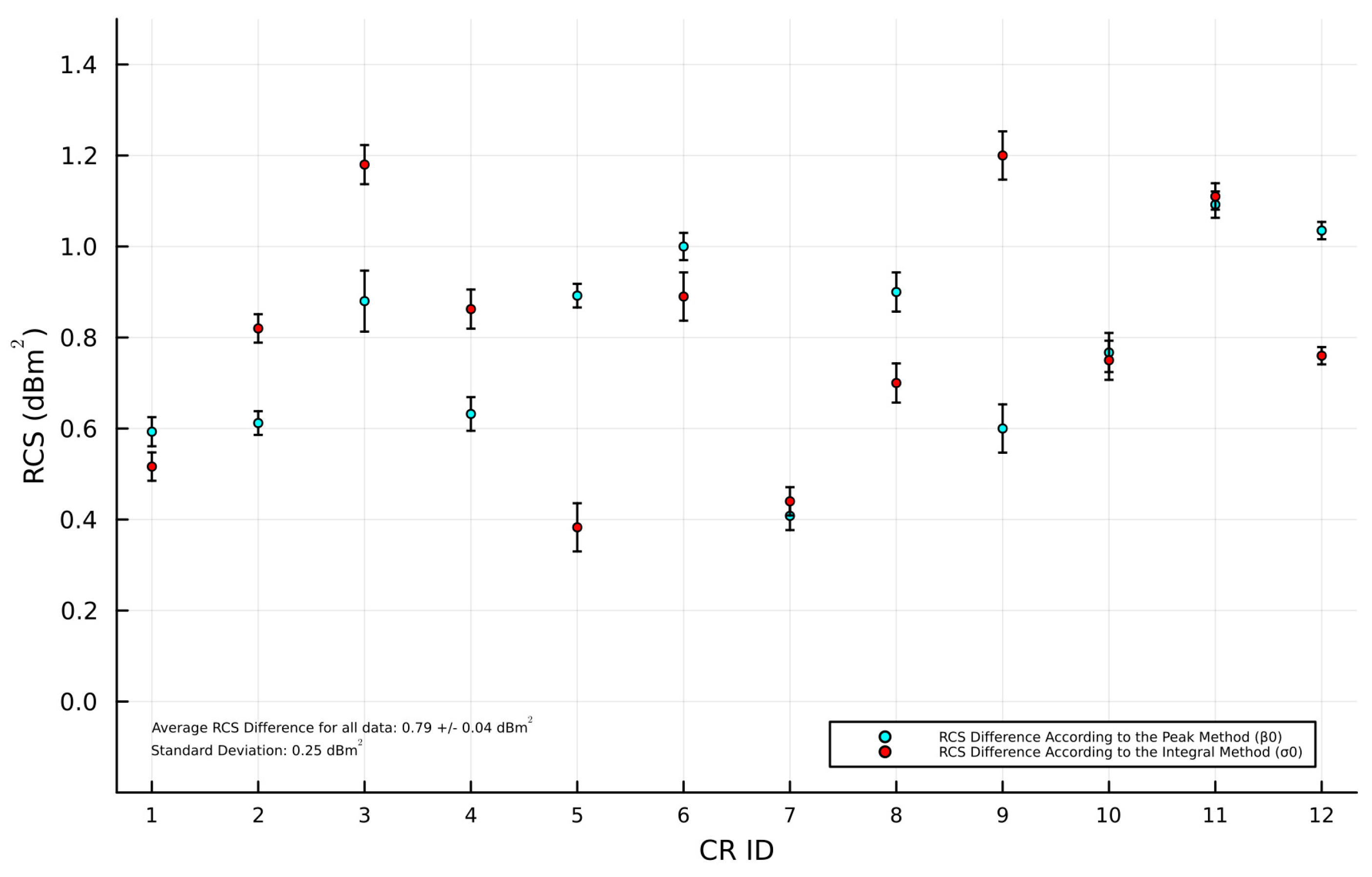
3.2. RCS and SCR Estimation
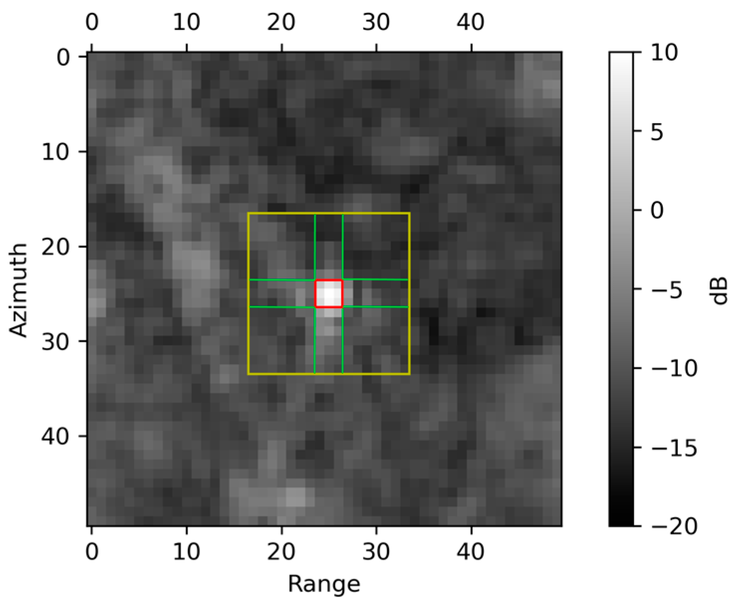
3.2.1. Integral Method
3.2.2. Peak Method
3.2.3. Displacement Error in LoS
3.2.4. Expected Localization Limits
3.2.5. Absolute Location Error
4. Discussion
5. Conclusions
Author Contributions
Funding
Data Availability Statement
Acknowledgments
Conflicts of Interest
Appendix A. Image Quality Performance


Appendix B. RCS and SCR Estimations


References
- Danezis, C.; Kakoullis, D.; Fotiou, K.; Pekri, M.; Chatzinikos, M.; Kotsakis, C.; Brcic, R.; Eineder, M.; Nikolaidis, M.; Ioannou, G.; et al. CyCLOPS: A National Integrated GNSS/InSAR Strategic Research Infrastructure for Monitoring Geohazards and Forming the Next Generation Datum of the Republic of Cyprus. In Geodesy for a Sustainable Earth. International Association of Geodesy Symposia; Freymueller, J.T., Sánchez, L., Eds.; Springer: Cham, Switzerland, 2022; Volume 154. [Google Scholar]
- Garthwaite, M.C.; Hazelwood, M.; Nancarrow, S.; Hislop, A.; Dawson, J.H. A Regional Geodetic Network to Monitor Ground Surface Response to Resource Extraction in the Northern Surat Basin, Queensland. Aust. J. Earth Sci. 2015, 62, 469–477. [Google Scholar] [CrossRef]
- Freeman, A. SAR Calibration: An Overview. IEEE Trans. Geosci. Remote Sens. 1992, 30, 1107–1121. [Google Scholar] [CrossRef]
- ESA External Calibration. Available online: https://sentinels.copernicus.eu/web/sentinel/technical-guides/sentinel-1-sar/cal-val-activities/calibration/external (accessed on 6 April 2023).
- Mahapatra, P.; Marel, H.; Van Leijen, F.; Samiei Esfahany, S.; Klees, R.; Hanssen, R. InSAR Datum Connection Using GNSS-Augmented Radar Transponders. J. Geod. 2017, 92, 21–32. [Google Scholar] [CrossRef]
- Kakoullis, D.; Fotiou, K.; Melillos, G.; Danezis, C. Considerations and Multi-Criteria Decision Analysis for the Installation of Collocated Permanent GNSS and SAR Infrastructures for Continuous Space-Based Monitoring of Natural Hazards. Remote Sens. 2022, 14, 1020. [Google Scholar] [CrossRef]
- IGS. IGS Site Guidelines; Infrastructure Commitee, Central Bureau: Pasadena, CA, USA, 2015.
- NGS. Guidelines for New and Existing Continuously Operating Reference Stations (CORS); NOAA: Washington, DC, USA; Silver Spring: Montgomery County, ML, USA, 2018; p. 21. [Google Scholar]
- EUREF Permanent GNSS Network Central Bureau Guidelines for EPN Stations and Operational Centres. 2022. Available online: https://www.epncb.oma.be/DOI/ROB-EUREF-Guidelines-Station.php (accessed on 4 July 2022).
- Garthwaite, M.C.; Lawrie, S.; Dawson, J.; Thankappan, M. Corner Reflectors as the Tie between InSAR and GNSS Measurements: Case Study of Resource Extraction in Australia. In Proceedings of the Fringe 2015: Advances in the Science and Applications of SAR Interferometry and Sentinel-1 InSAR Workshop, Frascati, Italy, 23–27 March 2015. [Google Scholar]
- Parker, A.L.; Featherstone, W.E.; Penna, N.T.; Filmer, M.S.; Garthwaite, M.C. Practical Considerations before Installing Ground-Based Geodetic Infrastructure for Integrated InSAR and cGNSS Monitoring of Vertical Land Motion. Sensors 2017, 17, 1753. [Google Scholar] [CrossRef]
- Thankappan, M.; Garthwaite, M.C.; Williams, M.L.; Hislop, A.; Nancarrow, S.; Dawson, J. Characterisation of Corner Reflectors for the Australian Geophysical Observing System to Support SAR Calibration. In Proceedings of the ResearchGate, Edinburgh, UK, 9 September 2013. [Google Scholar]
- Freeman, A. Radiometric calibration of SAR image data. ISPRS J. Photogramm. Remote Sens. 1993, XXIX, 212–222. [Google Scholar]
- Sharma, S.; Dadhich, G.; Rambhia, M.; Mathur, A.K.; Prajapati, R.P.; Patel, P.R.; Shukla, A. Radiometric Calibration Stability Assessment for the RISAT-1 SAR Sensor Using a Deployed Point Target Array at the Desalpar Site, Rann of Kutch, India. Int. J. Remote Sens. 2017, 38, 7242–7259. [Google Scholar] [CrossRef]
- Schubert, A.; Small, D.; Miranda, N.; Geudtner, D.; Meier, E. Sentinel-1A Product Geolocation Accuracy: Commissioning Phase Results. Remote Sens. 2015, 7, 9431–9449. [Google Scholar] [CrossRef]
- Gisinger, C.; Krieger, L.; Valentino, A.; Breit, H.; Albinet, C.; Eineder, M. ESA’s Extended Timing Annotation Dataset (ETAD) for Sentinel-1—Product Status and Case Studies. In Proceedings of the Living Planet Symposium 2022, Bonn, Germany, 23 May 2022. [Google Scholar]
- Schubert, A.; Small, D.; Meier, E.; Miranda, N.; Geudtner, D. Spaceborne SAR Product Geolocation Accuracy: A Sentinel-1 Update. In Proceedings of the 2014 IEEE Geoscience and Remote Sensing Symposium, Quebec City, QC, Canada, 13–18 July 2014; pp. 2675–2678. [Google Scholar]
- ESA Mission Ends for Copernicus Sentinel-1B Satellite. Available online: https://www.esa.int/Applications/Observing_the_Earth/Copernicus/Sentinel-1/Mission_ends_for_Copernicus_Sentinel-1B_satellite (accessed on 4 July 2022).
- ESA Sentinel-1 Data Products. Available online: https://www.esa.int/Applications/Observing_the_Earth/Copernicus/Sentinel-1/Data_products (accessed on 31 August 2023).
- ESA SAR Product Types. Available online: https://copernicus.eu/user-guides/sentinel-1-sar/product-types-processing-levels/level-1 (accessed on 31 August 2023).
- Facility Alaska Satellite Sentinel-1—Observation Plans. Available online: https://asf.alaska.edu/data-sets/sar-data-sets/sentinel-1/sentinel-1-observation-plans/ (accessed on 1 March 2024).
- De Zan, F.; Monti Guarnieri, A. TOPSAR: Terrain Observation by Progressive Scans. IEEE Trans. Geosci. Remote Sens. 2006, 44, 2352–2360. [Google Scholar] [CrossRef]
- Knott, E.F. Radar Cross Section Measurements; Springer Science and Business Media: Berlin/Heidelberg, Germany, 2012; ISBN 978-1-4684-9904-9. [Google Scholar]
- Garthwaite, M.C.; Nancarrow, S.; Hislop, A.; Thankappan, M.; Dawson, J.H.; Lawrie, S. The Design of Radar Corner Reflectors for the Australian Geophysical Observing System: A Single Design Suitable for InSAR Deformation Monitoring and SAR Calibration at Multiple Microwave Frequency Bands; Geoscience Australia: Canberra, Australia, 2015; ISBN 978-1-925124-57-6.
- Miranda, N.; Meadows, P.J. Radiometric Calibration of S-1 Level-1 Products Generated by the S-1 IPF 2015. Available online: https://sentinel.esa.int/documents/247904/685163/S1-Radiometric-Calibration-V1.0.pdf (accessed on 4 July 2022).
- Czikhardt, R.; Van Der Marel, H.; Papco, J. GECORIS: An Open-Source Toolbox for Analyzing Time Series of Corner Reflectors in InSAR Geodesy. Remote Sens. 2021, 13, 926. [Google Scholar] [CrossRef]
- Atwood, D.; Small, D.; Gens, R. Improving PolSAR Land Cover Classification With Radiometric Correction of the Coherency Matrix. IEEE J. Sel. Top. Appl. Earth Obs. Remote Sens. 2012, 5, 848–856. [Google Scholar] [CrossRef]
- Brock, B.; Doerry, A. Radar Cross Section of Triangular Trihedral Reflector with Extended Bottom Plate; U.S. Department of Commerce, National Techical Information Service: Springfield, VA, USA, 2009.
- Garthwaite, M.C. On the Design of Radar Corner Reflectors for Deformation Monitoring in Multi-Frequency InSAR. Remote Sens. 2017, 9, 648. [Google Scholar] [CrossRef]
- Qin, Y.; Perissin, D.; Lei, L. The Design and Experiments on Corner Reflectors for Urban Ground Deformation Monitoring in Hong Kong. Int. J. Antennas Propag. 2013, 2013, 191685. [Google Scholar] [CrossRef]
- Jauvin, M.; Yan, Y.; Trouvé, E.; Fruneau, B.; Gay, M.; Girard, B. Integration of Corner Reflectors for the Monitoring of Mountain Glacier Areas with Sentinel-1 Time Series. Remote Sens. 2019, 11, 988. [Google Scholar] [CrossRef]
- Bamler, R.; Hartl, P. Synthetic Aperture Radar Interferometry. Inverse Probl. 1998, 14, R1. [Google Scholar] [CrossRef]
- Czikhardt, R.; van der Marel, H.; van Leijen, F.J.; Hanssen, R.F. Estimating Signal-to-Clutter Ratio of InSAR Corner Reflectors From SAR Time Series. IEEE Geosci. Remote Sens. Lett. 2022, 19, 4012605. [Google Scholar] [CrossRef]
- Carsey, F.D. Microwave Remote Sensing of Sea Ice; American Geophysical Union: Washington, DC, USA, 1992; ISBN 978-0-87590-033-9. [Google Scholar]
- Bourbigot, M. Sentinel-1 Product Definition 2016. Available online: https://sentinels.copernicus.eu/documents/247904/1877131/Sentinel-1-Product-Definition.pdf/6049ee42-6dc7-4e76-9886-f7a72f5631f3?t=1461673251000 (accessed on 4 July 2022).
- Andersson, F.; Moses, R.; Natterer, F. Fast Fourier Methods for Synthetic Aperture Radar Imaging. IEEE Trans. Aerosp. Electron. Syst. 2012, 48, 215–229. [Google Scholar] [CrossRef]
- Tienda, C.; Bertl, N.; Younis, M.; Krieger, G. Characterization of the Cross-Talk SAR Image Produced by the Cross-Polarization in a Single Offset Parabolic Reflector. In Proceedings of the 2015 9th European Conference on Antennas and Propagation (EuCAP), Lisbon, Portugal, 13–17 April 2015; pp. 1–4. [Google Scholar]
- Dadhich, G.; Sharma, S.; Rambhia, M.; Mathur, A.K.; Patel, P.R.; Shukla, A. Image Quality Characterization of Fine Resolution RISAT-1 Data Using Impulse Response Function. Geocarto Int. 2019, 34, 586–596. [Google Scholar] [CrossRef]
- Small, D. Flattening Gamma: Radiometric Terrain Correction for SAR Imagery. IEEE Trans. Geosci. Remote Sens. 2011, 49, 3081–3093. [Google Scholar] [CrossRef]
- Vu, V.T.; Sjögren, T.K.; Pettersson, M.I.; Gustavsson, A. Definition on SAR Image Quality Measurements for UWB SAR. In Image and Signal Processing for Remote Sensing XIV; SPIE: Bellingham, WA, USA, 2008; Volume 7109, pp. 367–375. [Google Scholar]
- Martínez, A.; Marchand, J.L. SAR Image Quality Assessment. Rev. Teledetec. 1993, 2, 12–18. [Google Scholar]
- Schwerdt, M.; Schmidt, K.; Tous Ramon, N.; Klenk, P.; Yague-Martinez, N.; Prats-Iraola, P.; Zink, M.; Geudtner, D. Independent System Calibration of Sentinel-1B. Remote Sens. 2017, 9, 511. [Google Scholar] [CrossRef]
- Gray, A.L.; Vachon, P.W.; Livingstone, C.E.; Lukowski, T.I. Synthetic Aperture Radar Calibration Using Reference Reflectors. IEEE Trans. Geosci. Remote Sens. 1990, 28, 374–383. [Google Scholar] [CrossRef]
- Li, C.; Zhao, J.; Yin, J.; Zhang, G.; Shan, X. Analysis of RCS Characteristic of Dihedral Corner and Triangular Trihedral Corner Reflectors. In Proceedings of the 2010 5th International Conference on Computer Science Education, Hefei, China, 24–27 August 2010; pp. 40–43. [Google Scholar]
- Ulander, I.M.H. Accuracy of Using Point Targets for SAR Calibration. IEEE Trans. Aerosp. Electron. Syst. 1991, 27, 139–148. [Google Scholar] [CrossRef]
- Praveen, T.N.; Vinod Raju, M.; Vishwanath, B.D.; Meghana, P.; Manjula, T.R.; Raju, G. Absolute Radiometric Calibration of RISAT-1 SAR Image Using Peak Method. In Proceedings of the 2018 3rd IEEE International Conference on Recent Trends in Electronics, Information & Communication Technology (RTEICT), Bangalore, India, 18–19 May 2018; pp. 456–460. [Google Scholar]
- Ketelaar, G.; Marinkovic, P.; Hanssen, R. Validation of Point Scatterer Phase Statistics in Multi-Pass InSAR. In Envisat & ERS Symposium; ESA Special Publication; ESA: Salzburg, Austria, 2005; Volume 572, p. 72.1. [Google Scholar]
- Dawson, J. Satellite Radar Interferometry with Application to the Observation of Surface Deformation in Australia; The Australian National University: Canberra, Australia, 2008. [Google Scholar]
- Ferretti, A.; Savio, G.; Barzaghi, R.; Borghi, A.; Musazzi, S.; Novali, F.; Prati, C.; Rocca, F. Submillimeter Accuracy of InSAR Time Series: Experimental Validation. IEEE Trans. Geosci. Remote Sens. 2007, 45, 1142–1153. [Google Scholar] [CrossRef]
- Balss, U.; Gisinger, C.; Eineder, M. Measurements on the Absolute 2-D and 3-D Localization Accuracy of TerraSAR-X. Remote Sens. 2018, 10, 656. [Google Scholar] [CrossRef]
- Gisinger, C.; Schubert, A.; Breit, H.; Garthwaite, M.; Balss, U.; Willberg, M.; Small, D.; Eineder, M.; Miranda, N. In-Depth Verification of Sentinel-1 and TerraSAR-X Geolocation Accuracy Using the Australian Corner Reflector Array. IEEE Trans. Geosci. Remote Sens. 2021, 59, 1154–1181. [Google Scholar] [CrossRef]
- Gisinger, C.; Libert, L.; Marinkovic, P.; Krieger, L.; Larsen, Y.; Valentino, A.; Breit, H.; Balss, U.; Suchandt, S.; Nagler, T.; et al. The Extended Timing Annotation Dataset for Sentinel-1—Product Description and First Evaluation Results. IEEE Trans. Geosci. Remote Sens. 2022, 60, 5232622. [Google Scholar] [CrossRef]
- Balss, U.; Gisinger, C.; Eineder, M.; Breit, H.; Schubert, A.; Small, D. Survey Protocol for Geometric SAR Sensor Analysis; ESRIN: Frascati, Italy, 2018. [Google Scholar]
- Small, D.; Schubert, A. Guide to Sentinel-1 Geocoding; RSL, UZH, 2022; p. 42. Available online: https://sentinel.esa.int/documents/247904/1653442/Guide-to-Sentinel-1-Geocoding.pdf (accessed on 22 February 2024).
- Wegmuller, U.; Werner, C. GAMMA SAR Processor and Interferometry Software. In Proceedings of the 3rd ERS Scientific Symposium, Florencen, Italy, 17 March 1997. [Google Scholar]
- ASF ASF Data Search. Available online: https://search.asf.alaska.edu/#/ (accessed on 22 February 2024).
- Calabrese, D.; Episcopo, R. Derivation of the SAR Noise Equivalent Sigma Nought. In Proceedings of the EUSAR 2014: 10th European Conference on Synthetic Aperture Radar, Berlin, Germany, 3–5 June 2014; pp. 1–4. [Google Scholar]
- Department of Meteorology Climatological Information. Available online: https://www.moa.gov.cy/moa/dm/dm.nsf/home_en/home_en?openform (accessed on 19 January 2024).
- Hanssen, R.F. Radar Interferometry: Data Interpretation and Error Analysis; Springer Science and Business Media: Berlin/Heidelberg, Germany, 2001; ISBN 978-0-7923-6945-5. [Google Scholar]
- Hersbach, H.; Bell, B.; Berrisford, P.; Hirahara, S.; Horányi, A.; Muñoz-Sabater, J.; Nicolas, J.; Peubey, C.; Radu, R.; Schepers, D.; et al. The ERA5 Global Reanalysis. Q. J. R. Meteorol. Soc. 2020, 146, 1999–2049. [Google Scholar] [CrossRef]
- Eineder, M.; Minet, C.; Steigenberger, P.; Cong, X.; Fritz, T. Imaging Geodesy—Toward Centimeter-Level Ranging Accuracy With TerraSAR-X. IEEE Trans. Geosci. Remote Sens. 2011, 49, 661–671. [Google Scholar] [CrossRef]
- Cong, X.; Balss, U.; Eineder, M.; Fritz, T. Imaging Geodesy—Centimeter-Level Ranging Accuracy With TerraSAR-X: An Update. IEEE Geosci. Remote Sens. Lett. 2012, 9, 948–952. [Google Scholar] [CrossRef]


| Parameters | IW1 | IW2 | IW3 |
|---|---|---|---|
| * PSLR in range and azimuth [dB] | <−21.2 | ||
| * ISLR in range and azimuth [dB] | <−16.1 | ||
| Slant Range Resolution [m] | 2.7 | 3.1 | 3.5 |
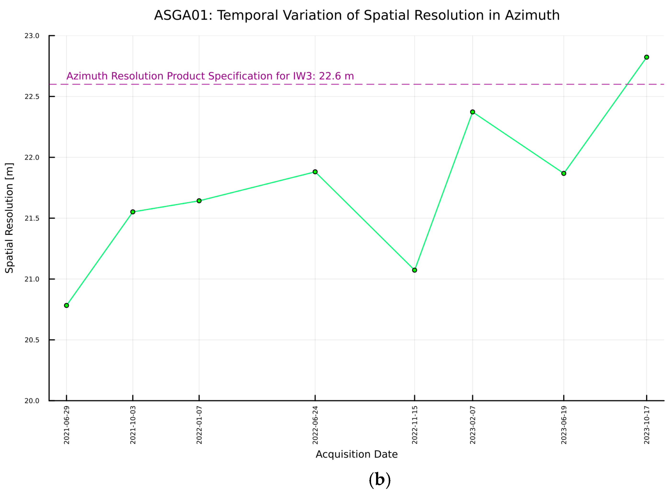
| Azimuth Resolution [m] | 22.5 | 22.7 | 22.6 |
| Range [m] | Azimuth [m] | |
|---|---|---|
| IW1 | ||
| Mean | 2.7 | 21.9 |
| St. Deviation | 0.09 | 0.5 |
| Max | 2.8 | 22.8 |
| Min | 2.5 | 20.8 |
| IW2 | ||
| Mean | 3.1 | 22.1 |
| St. Deviation | 0.09 | 0.6 |
| Max | 3.3 | 23.5 |
| Min | 2.9 | 21.2 |
| IW3 | ||
| Mean | 3.5 | 21.8 |
| St. Deviation | 0.09 | 0.5 |
| Max | 3.7 | 22.8 |
| Min | 3.4 | 20.8 |
| Range [dB] | Azimuth [dB] | |
|---|---|---|
| Mean | −19.3 | −20.2 |
| St. Deviation | 2.2 | 3.4 |
| Max | −15 | −13.6 |
| Min | −25.8 | −34.8 |
| Product | Rel. Orbit No. | Frame | Mode | Pixel Spacing (rg × az) [m] | Spatial Resolution (rg × az) [m] | No. of Looks | Coordinate System |
|---|---|---|---|---|---|---|---|
| SLC | 160, 167 | 107, 112, 476 | IW | 2.3 × 14.1 | 2.7 × 22 to 3.5 × 22 | 1 | Slant Range × Azimuth |
| GRD | 160, 167 | 107, 112, 476 | IW | H 10 × 10 | H 20 × 22 | 5 × 1 | Ground Range × Azimuth |
| Code No. | ID | Mean RCS ± 1σ | Standard Deviation | Diff. from RCST |
|---|---|---|---|---|
| 1 | SOUN01 | 37.9 ± 0.04 | ±0.3 | 0.5 |
| 2 | AKMS01 | 37.6 ± 0.05 | ±0.3 | 0.8 |
| 3 | ALEV01 | 37.3 ± 0.06 | ±0.4 | 1.1 |
| 4 | ASGA01 | 37.6 ± 0.04 | ±0.3 | 0.8 |
| 5 | MATS01 | 38 ± 0.03 | ±0.2 | 0.4 |
| 6 | TROU01 | 37.5 ± 0.06 | ±0.4 | 0.9 |
| 7 | SOUN02 | 38 ± 0.03 | ±0.2 | 0.4 |
| 8 | AKMS02 | 37.7 ± 0.04 | ±0.3 | 0.7 |
| 9 | ALEV02 | 37.2 ± 0.07 | ±0.5 | 1.2 |
| 10 | ASGA02 | 37.7 ± 0.06 | ±0.5 | 0.7 |
| 11 | MATS02 | 37.3 ± 0.05 | ±0.4 | 1.1 |
| 12 | TROU02 | 37.6 ± 0.04 | ±0.3 | 0.7 |
| Code No. | ID | Mean RCS before Realignment | Mean RCS after Realignment |
|---|---|---|---|
| 3 | ALEV01 | 36.4 ± 0.05 | 37.5 ± 0.06 |
| 8 | AKMS02 | 37.4 ± 0.04 | 38.2 ± 0.03 |
| 9 | ALEV02 | 36.3 ± 0.07 | 37.8 ± 0.05 |
| Code No. | ID | Mean RCS ± 1σ | Standard Deviation | Diff. from RCST |
|---|---|---|---|---|
| 1 | SOUN01 | 37.8 ± 0.03 | ±0.3 | 0.6 |
| 2 | AKMS01 | 37.8 ± 0.03 | ±0.2 | 0.6 |
| 3 | ALEV01 | 37.5 ± 0.06 | ±0.5 | 0.9 |
| 4 | ASGA01 | 37.8 ± 0.04 | ±0.3 | 0.6 |
| 5 | MATS01 | 37.5 ± 0.03 | ±0.2 | 0.9 |
| 6 | TROU01 | 37.4 ± 0.03 | ±0.2 | 1.0 |
| 7 | SOUN02 | 38.0 ± 0.03 | ±0.2 | 0.4 |
| 8 | AKMS02 | 37.5 ± 0.04 | ±0.3 | 0.9 |
| 9 | ALEV02 | 37.8 ± 0.05 | ±0.6 | 0.6 |
| 10 | ASGA02 | 37.6 ± 0.04 | ±0.3 | 0.8 |
| 11 | MATS02 | 37.3 ± 0.03 | ±0.2 | 1.1 |
| 12 | TROU02 | 37.3 ± 0.02 | ±0.2 | 1.1 |
| TTCR | SCR [dB] | Location Accuracy [Res. Cells] | Expected Localization Accuracy | |
|---|---|---|---|---|
| Range [m] | Azimuth [m] | |||
| SOUN01 | 28.7 | 0.014 | 0.044 | 0.298 |
| AKMS01 | 29.6 | 0.013 | 0.040 | 0.269 |
| ALEV01 | 22.0 | 0.031 | 0.096 | 0.644 |
| ASGA01 | 27.0 | 0.017 | 0.061 | 0.380 |
| MATS01 | 29.4 | 0.013 | 0.046 | 0.288 |
| TROU01 | 29.4 | 0.013 | 0.046 | 0.288 |
| SOUN02 | 29.0 | 0.014 | 0.043 | 0.288 |
| AKMS02 | 24.5 | 0.023 | 0.072 | 0.483 |
| ALEV02 | 21.3 | 0.034 | 0.104 | 0.698 |
| ASGA02 | 27.7 | 0.016 | 0.043 | 0.352 |
| MATS02 | 27.9 | 0.016 | 0.042 | 0.344 |
| TROU02 | 27.6 | 0.016 | 0.044 | 0.356 |
| TTCR ID | Range ALE [m] | Azimuth ALE [m] | Difference from the Expected Accuracy (Expected-|ALE|) | |
|---|---|---|---|---|
| Range [m] | Azimuth [m] | |||
| AKMS01 | −0.001 ± 0.039 | 0.154 ± 0.277 | (>) 0.043 | (>) 0.144 |
| AKMS02 | −0.051 ± 0.071 | −0.094 ± 0.509 | (>) 0.021 | (>) 0.389 |
| ALEV01 | 0.006 ± 0.096 | −0.011 ± 0.682 | (>) 0.090 | (>) 0.633 |
| ALEV02 | −0.029 ± 0.130 | −0.386 ± 0.925 | (>) 0.075 | (>) 0.312 |
| ASGA01 | 0.016 ± 0.060 | 0.134 ± 0.377 | (>) 0.045 | (>) 0.003 |
| ASGA02 | −0.021 ± 0.042 | −0.273 ± 0.347 | (>) 0.051 | (>) 0.079 |
| MATS01 | 0.025 ± 0.046 | −0.369 ± 0.286 | (>) 0.021 | (<) 0.081 |
| MATS02 | −0.041 ± 0.041 | −0.181 ± 0.330 | (>) 0.001 | (>) 0.163 |
| SOUN01 | 0.010 ± 0.044 | 0.333 ± 0.313 | (>) 0.034 | (<) 0.035 |
| SOUN02 | 0.009 ± 0.042 | −0.09 ± 0.304 | (>) 0.034 | (>) 0.193 |
| TROU01 | −0.029 ± 0.046 | −0.198 ± 0.287 | (>) 0.017 | (>) 0.090 |
| TROU02 | −0.043 ± 0.044 | −0.060 ± 0.194 | (>) 0.001 | (>) 0.296 |
Disclaimer/Publisher’s Note: The statements, opinions and data contained in all publications are solely those of the individual author(s) and contributor(s) and not of MDPI and/or the editor(s). MDPI and/or the editor(s) disclaim responsibility for any injury to people or property resulting from any ideas, methods, instructions or products referred to in the content. |
© 2024 by the authors. Licensee MDPI, Basel, Switzerland. This article is an open access article distributed under the terms and conditions of the Creative Commons Attribution (CC BY) license (https://creativecommons.org/licenses/by/4.0/).
Share and Cite
Kakoullis, D.; Fotiou, K.; Ibarrola Subiza, N.; Brcic, R.; Eineder, M.; Danezis, C. An Advanced Quality Assessment and Monitoring of ESA Sentinel-1 SAR Products via the CyCLOPS Infrastructure in the Southeastern Mediterranean Region. Remote Sens. 2024, 16, 1696. https://doi.org/10.3390/rs16101696
Kakoullis D, Fotiou K, Ibarrola Subiza N, Brcic R, Eineder M, Danezis C. An Advanced Quality Assessment and Monitoring of ESA Sentinel-1 SAR Products via the CyCLOPS Infrastructure in the Southeastern Mediterranean Region. Remote Sensing. 2024; 16(10):1696. https://doi.org/10.3390/rs16101696
Chicago/Turabian StyleKakoullis, Dimitris, Kyriaki Fotiou, Nerea Ibarrola Subiza, Ramon Brcic, Michael Eineder, and Chris Danezis. 2024. "An Advanced Quality Assessment and Monitoring of ESA Sentinel-1 SAR Products via the CyCLOPS Infrastructure in the Southeastern Mediterranean Region" Remote Sensing 16, no. 10: 1696. https://doi.org/10.3390/rs16101696