
Study on Spatialization and Spatial Pattern of Population Based on Multi-Source Data—A Case Study of the Urban Agglomeration on the North Slope of Tianshan Mountain in Xinjiang, China

Abstract
1. Introduction
2. Materials and Methods
2.1. Study Area and Data
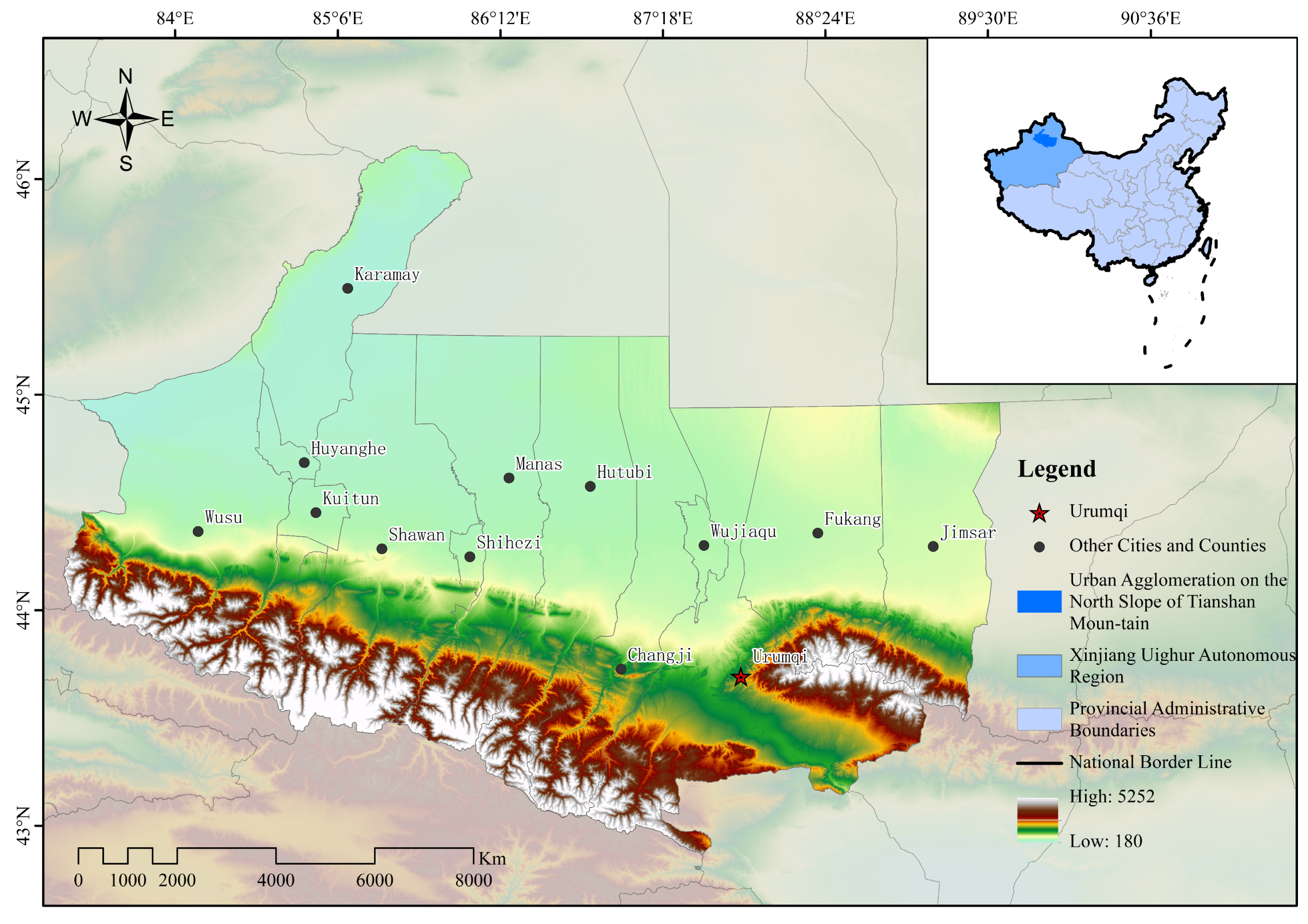
2.1.1. Study Area
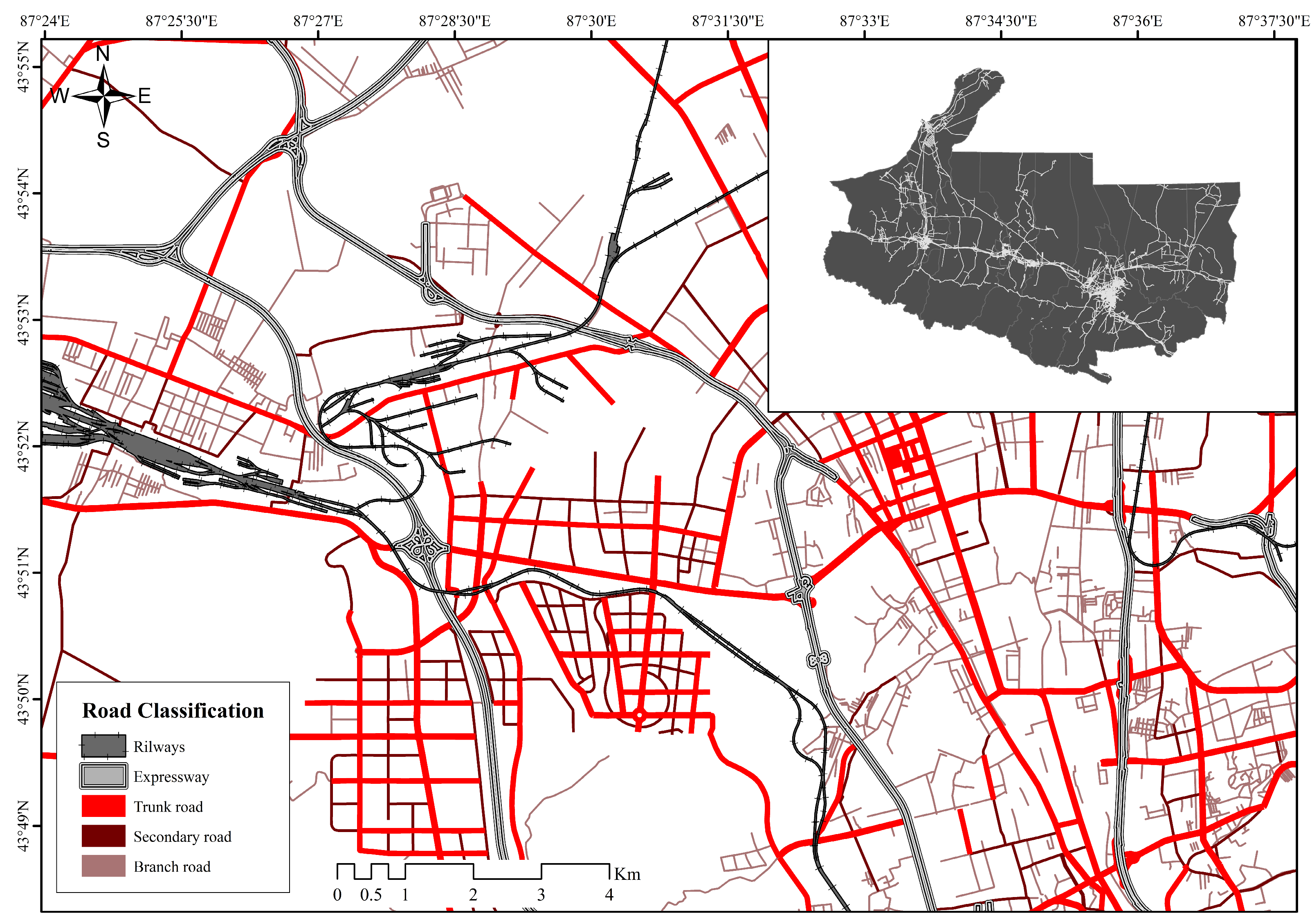
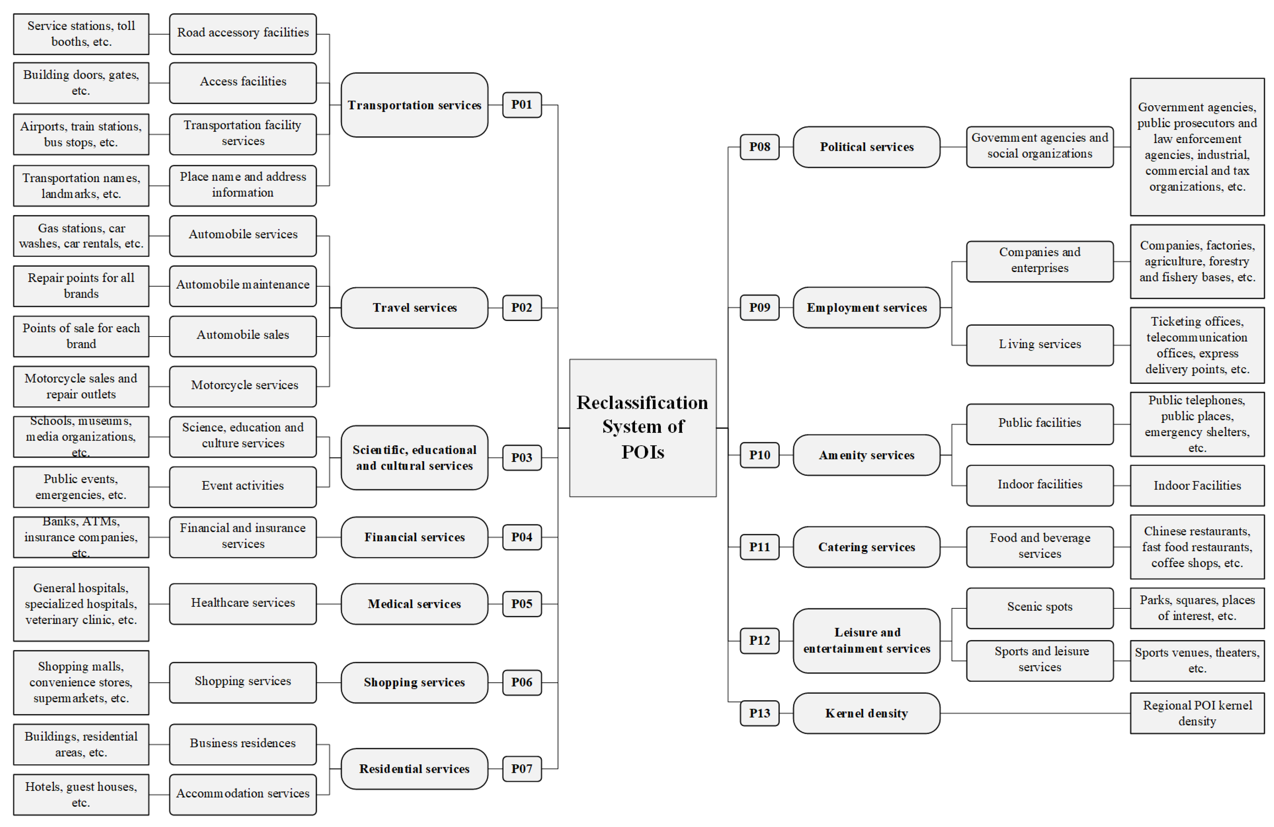
2.1.2. Data
2.2. Methods
2.2.1. Min–Max Standardization
2.2.2. Ordinary Least Square (OLS)
2.2.3. Pearson Correlation
2.2.4. Spatial Lag Model (SLM)
2.2.5. Random Forest Model (RFM)
2.2.6. Error Correction
2.2.7. Accuracy Verification
2.2.8. Standard Deviation Ellipse and Center of Gravity
2.2.9. Polycentricity
2.3. Database Indicator
2.3.1. Data Preprocessing
2.3.2. Significance and Covariance Diagnostics
3. Results
3.1. Spatialization of the Population
3.1.1. Spatial Autocorrelation Test
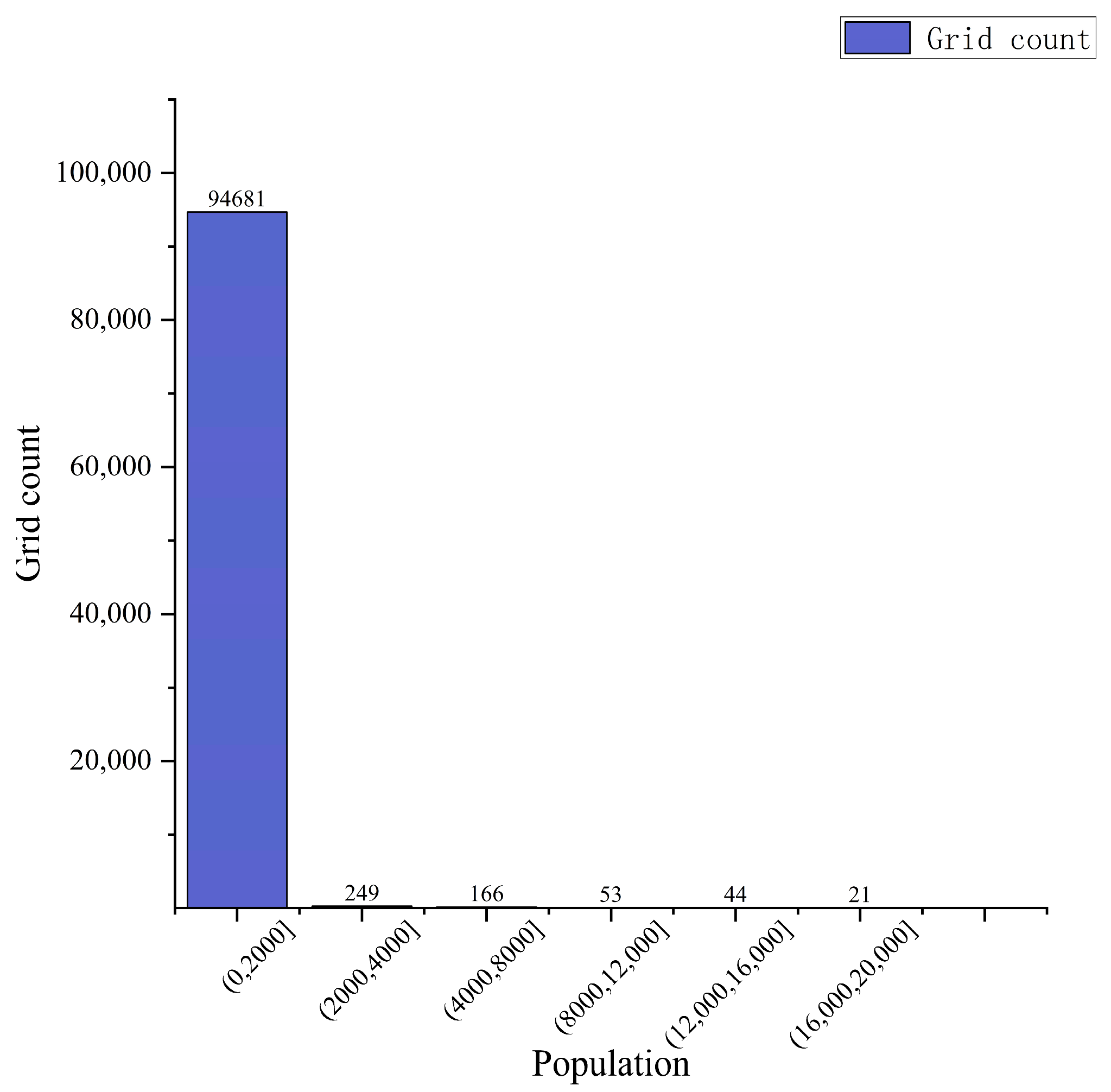
3.1.2. Construction of Population Spatialization Model Based on SLM
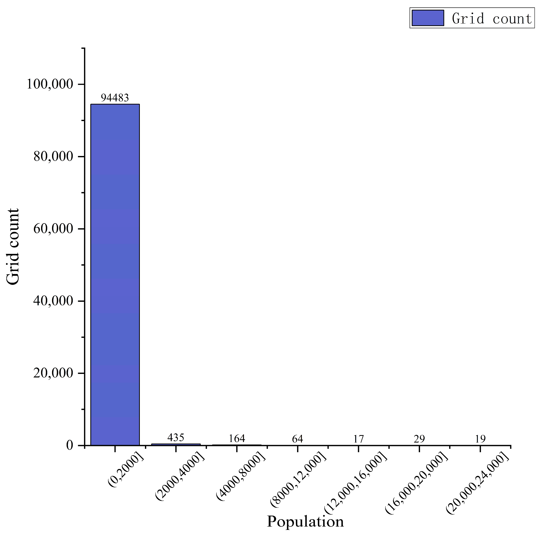
3.1.3. Construction of Population Spatialization Model Based on RFM
3.2. Accuracy Comparison
3.3. Patterns of Spatial Distribution of the Population
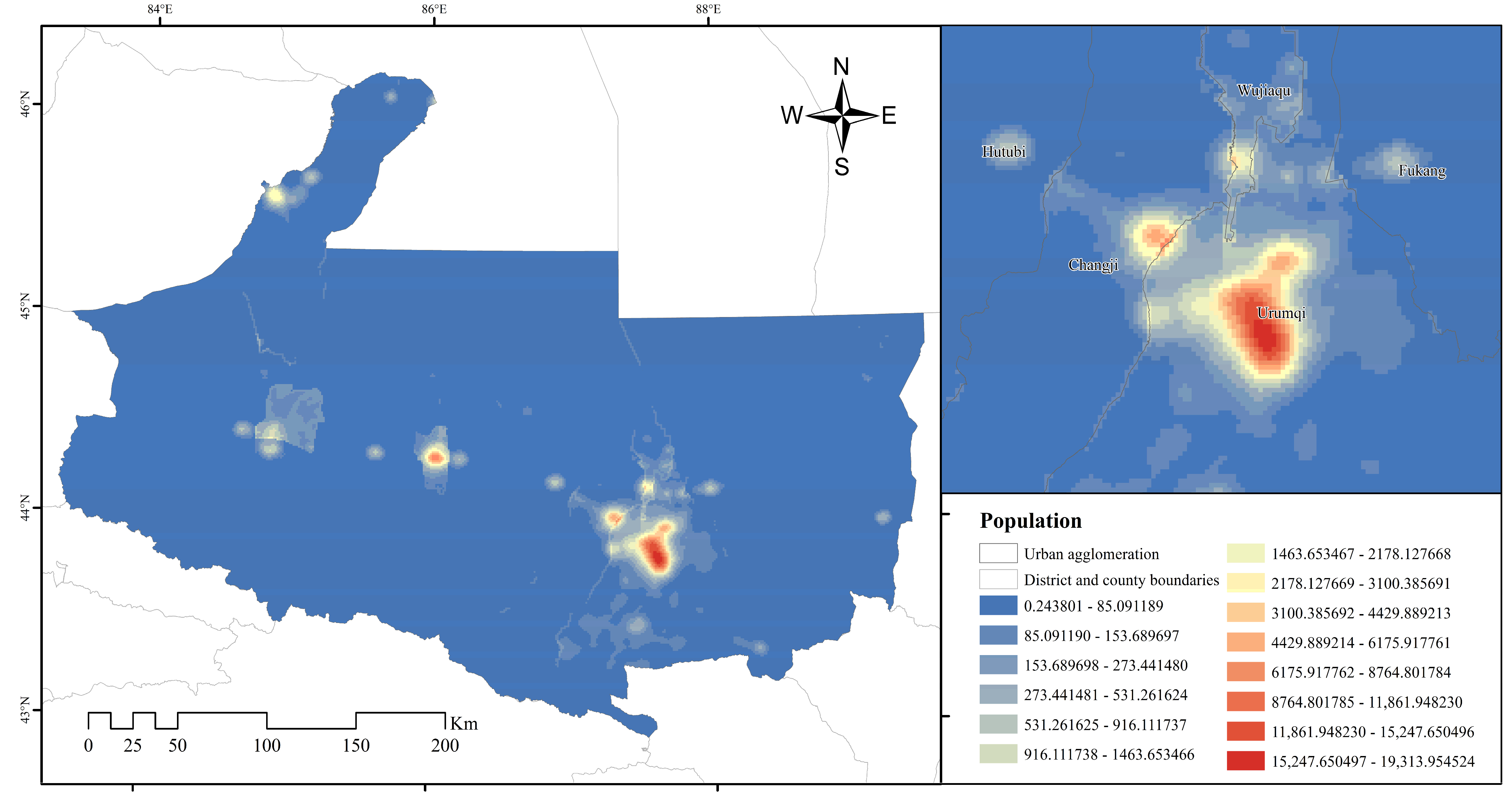
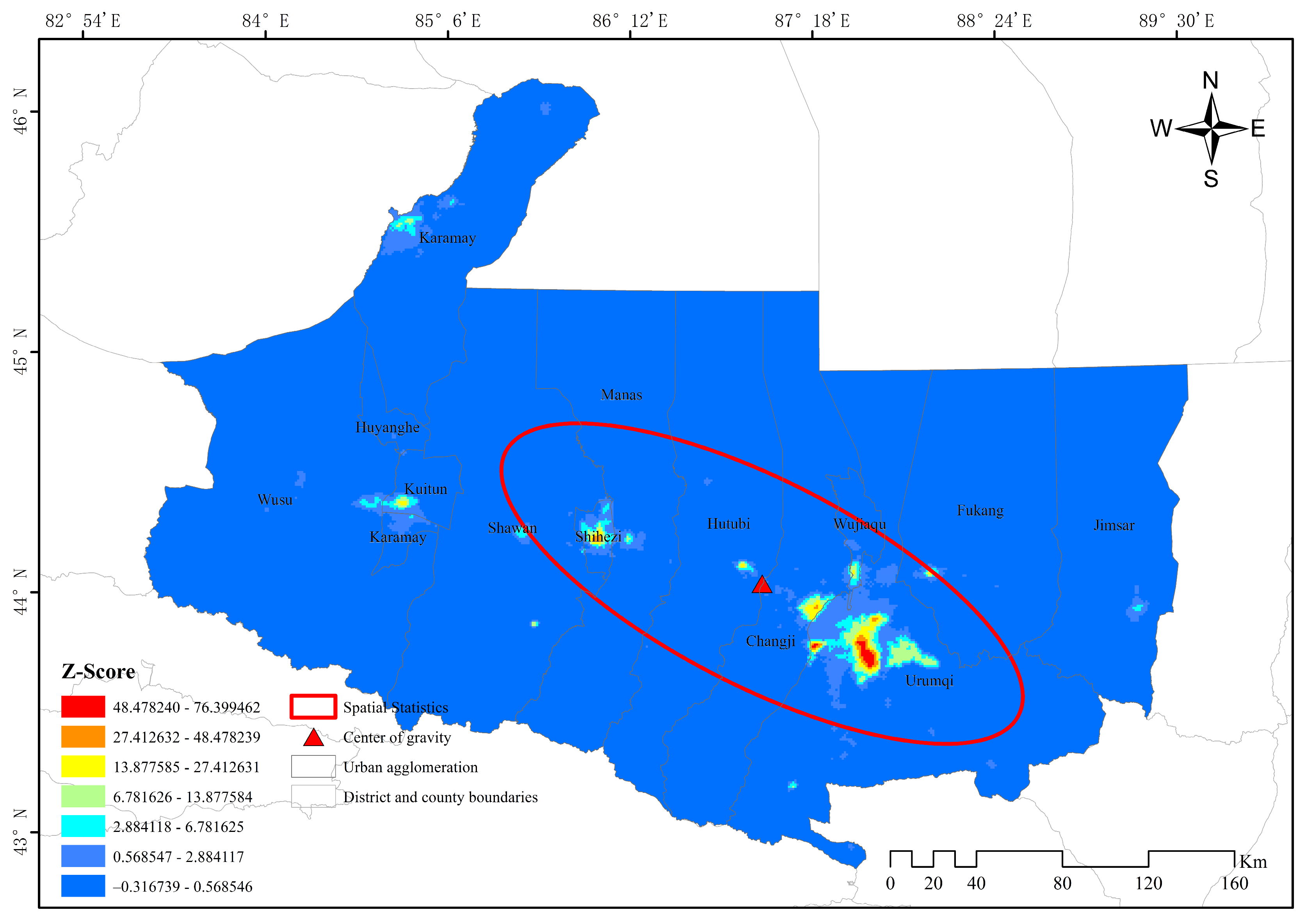
3.3.1. Cold and Hot Spots and Center of Gravity Distribution
3.3.2. Identification of Urban Agglomeration Centers
3.3.3. Exploration of Spatial Patterns of Population
4. Discussion
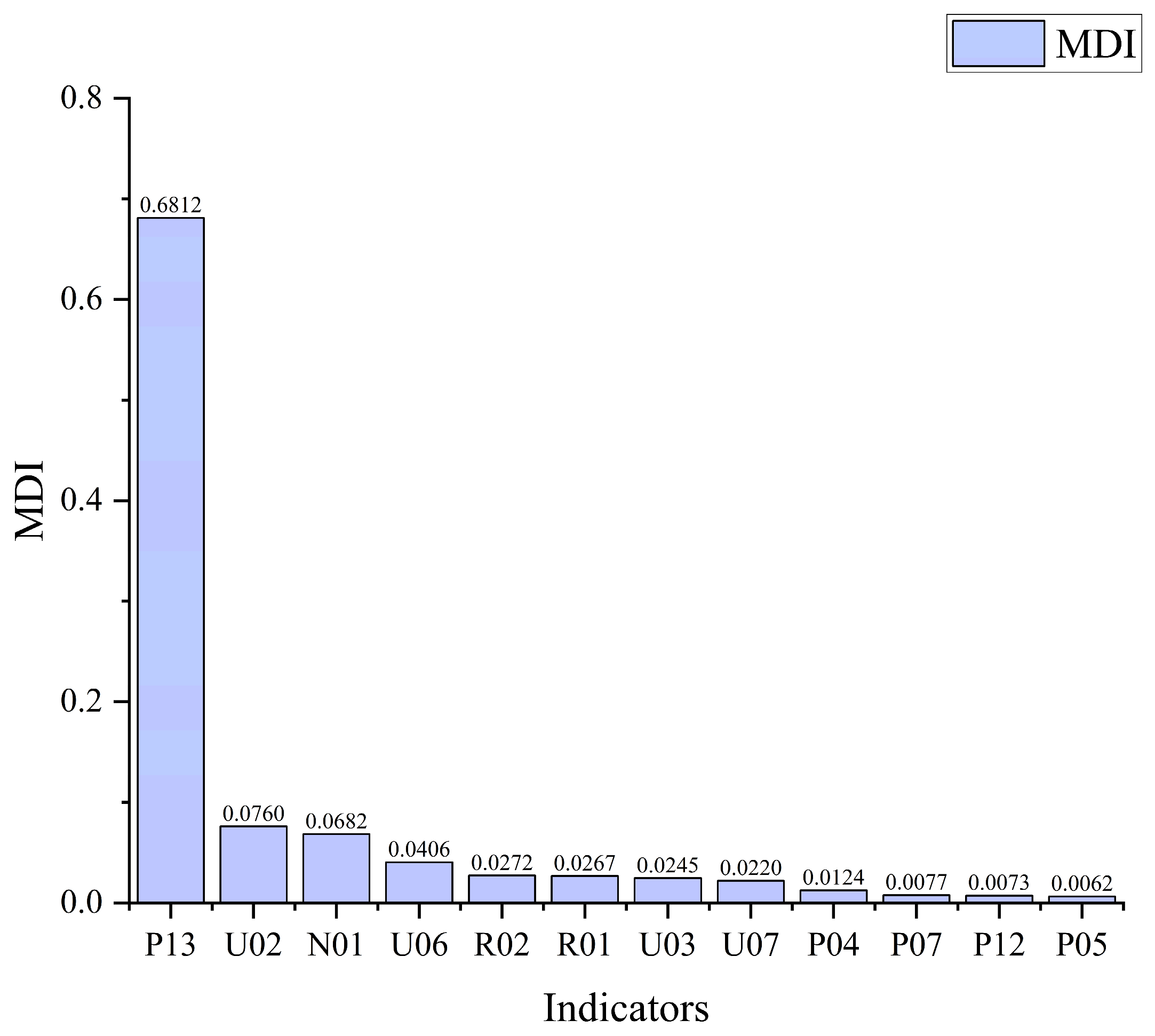
4.1. Feature Importance Analysis
4.2. Significance and Shortcomings
4.3. Recommendations
- Strengthen the radiating and driving effect: It is necessary to enhance the connection between the eastern and central–western parts of the urban agglomeration, further improve the information gathering and radiating capacity of the Urumqi–Shihezi–Kuitun–Karamay development axis both within and outside the region, strengthen the construction of transportation infrastructure, promote linkages between industries, and provide active guidance and support from the government to promote a more balanced and diversified new pattern of regional development.
- Coordinate regional communication and management: There is a need to strengthen the capacity for unified regional planning and management. Currently, there is a significant development gap between the “center” and “focal points” within the NSTS Urban Agglomeration. Further improvements in planning management and coordinated development mechanisms at various levels are required, with a focus on strengthening resource allocation towards peripheral cities, such as Wusu and Fukang, and accelerating the integration process.
- Strengthen internal industry collaboration: By encouraging cooperation between small- and medium-sized cities and the core city of Urumqi, an urban agglomeration structure with multiple active centers and extensive network connections should be constructed. Important linkages within the city network should be formed to optimize resource allocation and enhance the overall strength of the region. Ultimately, an economically strong, environmentally friendly, and culturally diverse urban agglomeration should be built.
- Respect the objective laws of development: Considering the characteristic of large spatial distances between cities and counties within the urban agglomeration, it is crucial to prevent the formulation of internal policies that detach from the actual economic development of the cities. Imitating the development paths of other large urban agglomerations blindly should be avoided. Instead, adapt to local geographic characteristics, setting new standards to measure the development status of the urban agglomeration, thus promoting sustainable regional development.
5. Conclusions
- The relative statistics of population under SLM simulation can show the spatial distribution of population more intuitively and effectively, but its actual performance has a more obvious near-circle layer structure.
- The spatial distribution of population under RFM simulation exhibits obvious spatial differentiation with irregular and expressive edges.
- SLM accuracy exceeds the two population raster datasets, GHS and GPW, with better accuracy but still needs improvement. RFM far exceeds the selected four types of datasets in terms of accuracy.
- The spatial pattern of the population of the NSTS Urban Agglomeration is mainly divided into four distinct circles, showing the distribution characteristics of “one center, multiple focal points”.
Author Contributions
Funding
Institutional Review Board Statement
Informed Consent Statement
Data Availability Statement
Acknowledgments
Conflicts of Interest
References
- Feng, Z.; Yang, Y.; You, Z.; Zhang, J. Research on the suitability of population distribution at the county level in China. Acta Geogr. Sin. 2014, 69, 723–737. [Google Scholar]
- Li, J.; Lu, D.; Xu, C.; Li, Y.; Chen, M. Spatial heterogeneity and its changes of population on the two sides of Hu Line. Acta Geogr. Sin. 2017, 72, 148–160. [Google Scholar]
- Ye, T.T.; Zhao, N.Z.; Yang, X.C.; Ouyang, Z.T.; Liu, X.P.; Chen, Q.; Hu, K.J.; Yue, W.Z.; Qi, J.G.; Li, Z.S.; et al. Improved population mapping for China using remotely sensed and points-of-interest data within a random forests model. Sci. Total Environ. 2019, 658, 936–946. [Google Scholar] [CrossRef] [PubMed]
- Chen, Z. Research on Demographic Statistical Data Spatialization Based on Residential Area Classifying. Geospat. Inf. 2016, 14, 47–48+52+47. [Google Scholar]
- Guo, H.; Zhu, W. A review on the spatial disaggregation of socioeconomic statistical data. Acta Geogr. Sin. 2022, 77, 2650–2667. [Google Scholar]
- Lung, T.; Lübker, T.; Ngochoch, J.K.; Schaab, G. Human population distribution modelling at regional level using very high resolution satellite imagery. Appl. Geogr. 2013, 41, 36–45. [Google Scholar] [CrossRef]
- He, M.; Xu, Y.M.; Li, N. Population Spatialization in Beijing City Based on Machine Learning and Multisource Remote Sensing Data. Remote Sens. 2020, 12, 1910. [Google Scholar] [CrossRef]
- Briggs, D.J.; Gulliver, J.; Fecht, D.; Vienneau, D.M. Dasymetric modelling of small-area population distribution using land cover and light emissions data. Remote Sens. Environ. 2007, 108, 451–466. [Google Scholar] [CrossRef]
- Zhuo, L.; Chen, J.; Shi, P.; Gu, Z.; Fan, Y.; Lchinose, T. Modeling Population Density of China in 1998 Based on DMSP/OLS Nighttime Light mage. Acta Geogr. Sin. 2005, 60, 266–276. [Google Scholar]
- Gao, Q.; Alimujiang, K.-S. Modeling the Population Spatial Distribution of Tianshan North-slope Urban Agglomeration Based on DMSP/OLS Night Lighting Data. Northwest Popul. J. 2017, 38, 113–120. [Google Scholar] [CrossRef]
- Li, H.; Zhang, H.; Wang, M. A Comparative Study of Population Spatialization Based on NPP/llRS and LJ1-01 Night Light Data:Taking Beijing for an Example. Remote Sens. Inf. 2021, 36, 90–97. [Google Scholar]
- Meiling, W.; Hesheng, Z. Research on Population Spatialization Based on Luojia-1 Nighttime Light Data. Geospat. Inf. 2021, 19, 53–56+57. [Google Scholar]
- Gaughan, A.E.; Stevens, F.R.; Linard, C.; Jia, P.; Tatem, A.J. High Resolution Population Distribution Maps for Southeast Asia in 2010 and 2015. PLoS ONE 2013, 8, e55882. [Google Scholar] [CrossRef]
- Ye, Q.; Yang, X.; Jiang, D. The Grid Scale Effect Analysis on Town leveled Population Statistical Data Spatialization. J. Geo-Inf. Sci. 2010, 12, 40–47. [Google Scholar] [CrossRef]
- Hu, L.J.; He, Z.Y.; Liu, J.P. Adaptive Multi-Scale Population Spatialization Model Constrained by Multiple Factors: A Case Study of Russia. Cartogr. J. 2017, 54, 265–282. [Google Scholar] [CrossRef]
- Zhuang, D.F.; Liu, M.L.; Deng, X.Z. Spatialization model of population based on dataset of land use and land cover change in China. Chin. Geogr. Sci. 2002, 12, 114–119. [Google Scholar] [CrossRef]
- Wang, K.; Cal, H.; Yang, X. Multiple scale spatialization of demographic data with multi-factor linear regression and geographically weighted regression models. Prog. Geogr. 2016, 35, 1494–1505. [Google Scholar]
- Xiong, J.N.; Li, K.; Cheng, W.M.; Ye, C.C.; Zhang, H. A Method of Population Spatialization Considering Parametric Spatial Stationarity: Case Study of the Southwestern Area of China. Isprs Int. J. Geo-Inf. 2019, 8, 495. [Google Scholar] [CrossRef]
- Tan, C.D.; Tang, Y.H.; Wu, X.F. Evaluation of the Equity of Urban Park Green Space Based on Population Data Spatialization: A Case Study of a Central Area of Wuhan, China. Sensors 2019, 19, 2929. [Google Scholar] [CrossRef]
- Guo, W.; Liu, J.K.; Zhao, X.S.; Hou, W.; Zhao, Y.X.; Li, Y.X.; Sun, W.B.; Fan, D.Q. Spatiotemporal dynamics of population density in China using nighttime light and geographic weighted regression method. Int. J. Digit. Earth 2023, 16, 2704–2723. [Google Scholar] [CrossRef]
- Chen, M.; Xian, Y.; Huang, Y.; Zhang, X.; Hu, M.; Guo, S.; Chen, L.; Liang, L. Fine-scale population spatialization data of China in 2018 based on real location-based big data. Sci. Data 2022, 9, 624. [Google Scholar] [CrossRef] [PubMed]
- Gao, P.; Wu, T.J.; Ge, Y.; Li, Z.H. Improving the accuracy of extant gridded population maps using multisource map fusion. Giscience Remote Sens. 2022, 59, 54–70. [Google Scholar] [CrossRef]
- Zhao, S.; Liu, Y.X.; Zhang, R.; Fu, B.J. China’s population spatialization based on three machine learning models. J. Clean. Prod. 2020, 256, 120644. [Google Scholar] [CrossRef]
- Chun, J.; Zhang, X.-C.; Huang, J.-F.; Zhang, P.-C. A Gridding Method of Redistributing Population Based on POls. Geogr. Geo-Inf. Sci. 2018, 34, 83–89+124+122. [Google Scholar]
- Li, K.N.; Chen, Y.H.; Li, Y. The Random Forest-Based Method of Fine-Resolution Population Spatialization by Using the International Space Station Nighttime Photography and Social Sensing Data. Remote Sens. 2018, 10, 1650. [Google Scholar] [CrossRef]
- Cui, X.; Zhang, J.; Wu, F.; Zhang, Q.; Wu, Y. Spatio-temporal Analysis of Population Dynamics based on Multi-source Data Integration for Beijing Municipal City. J. Geo-Inf. Sci. 2020, 22, 2199–2211. [Google Scholar]
- Mei, Y.; Gui, Z.; Wu, J.; Peng, D.; Li, R.; Wu, H.; Wei, Z. Population spatialization with pixel-level attribute grading by considering scale mismatch issue in regression modeling. Geo-Spat. Inf. Sci. 2022, 25, 365–382. [Google Scholar] [CrossRef]
- Peipei, D.; Xiyong, H. Spatial Simulation of Population in China’s Coastal Zone based on Multi-source Data. J. Geo-Inf. Sci. 2020, 22, 207–217. [Google Scholar]
- Wang, X.; Ning, X.; Zhang, H.; Wang, H.; Hao, M. Population spatialization by integrating LJ1-01 nighttime light and WeChat positioning data—Taking Beiiing city as an example. Sci. Surv. Mapp. 2022, 47, 173–183. [Google Scholar] [CrossRef]
- Guo, W.; Zhang, J.; Zhao, X.; Li, Y.; Liu, J.; Sun, W.; Fan, D. Combining Luojia1-01 Nighttime Light and Points-of-Interest Data for Fine Mapping of Population Spatialization Based on the Zonal Classification Method. IEEE J. Sel. Top. Appl. Earth Obs. Remote Sens. 2023, 16, 1589–1600. [Google Scholar] [CrossRef]
- Liu, Z. Research on Fine Population Spatialization Method Based on Multi-Source Geographic Data; Wuhan University: Wuhan, China, 2019; Available online: https://kns-cnki-net-s.webvpn.xju.edu.cn:8040/kcms2/article/abstract?v=FC2wxXHna7rhn0nl9d8IdtSskzdnzLE30RL0OFDmNKjUhWCyNMYWubAypu7MsyZCJXPkT3RaK4-XS5F9DI0CM_49anu0ivgowgTRD9MVcGEeekzGMC5B8136eIj0sZp37PhjpAXMQZo=&uniplatform=NZKPT&language=CHS (accessed on 12 December 2023).
- Zou, Y. Research on Population Spatialization Based on Multi-Source Data; China University of Mining and Technology: Beijing, China, 2020; Available online: https://link.cnki.net/doi/10.27623/d.cnki.gzkyu.2020.000269 (accessed on 12 December 2023).
- Bao, W.X.; Gong, A.D.; Zhao, Y.R.; Chen, S.Q.; Ba, W.R.; He, Y. High-Precision Population Spatialization In Metropolises Based On Ensemble Learning: A Case Study Of Beijing, China. Remote Sens. 2022, 14, 3654. [Google Scholar] [CrossRef]
- Sinha, P.; Gaughan, A.E.; Stevens, F.R.; Nieves, J.J.; Sorichetta, A.; Tatem, A.J. Assessing the spatial sensitivity of a random forest model: Application in gridded population modeling. Comput. Environ. Urban Syst. 2019, 75, 132–145. [Google Scholar] [CrossRef]
- Wang, Y.; Huang, C.; Zhao, M.; Hou, J.; Zhang, Y.; Gu, J. Mapping the Population Density in Mainland China Using Npp/Viirs And Points-of-Interest Data Based on a Random Forests Model. Remote Sens. 2020, 12, 3645. [Google Scholar] [CrossRef]
- Wang, M.; Wang, Y.; Li, B.; Cai, Z.; Kang, M. A Population Spatialization Model at the Building Scale Using Random Forest. Remote Sens. 2022, 14, 1811. [Google Scholar] [CrossRef]
- Jianjun, D.; Chunqiao, S.; Ruifan, L.; Guohua, Z. Spatial prediction of population based on random forest. In Proceedings of the 2022 IEEE 10th Joint International Information Technology and Artificial Intelligence Conference (ITAIC), Chongqing, China, 17–19 June 2022; Volume 10, pp. 1360–1363. [Google Scholar] [CrossRef]
- Liu, L.; Cheng, G.; Yang, J.; Cheng, Y. Population spatialization in Zhengzhou city based on multi-source data and random forest model. Front. Earth Sci. 2023, 11, 1092664. [Google Scholar] [CrossRef]
- Chen, Y.; Wang, S.; Gu, Z.; Yang, F. Modeling the Spatial Distribution of Population Based on Random Forest and Parameter Optimization Methods: A Case Study of Sichuan, China. Appl. Sci. 2024, 14, 446. [Google Scholar] [CrossRef]
- Liu, Y.; Yang, J.; Liu, Q. Study on Spatial Pattern of Population Development in Chinaan Empirical Study Based on the Data of the Seventh National Census. Stat. Decis. 2024, 40, 78–82. [Google Scholar] [CrossRef]
- Wang, H.; Zhang, W.; Song, H.; Yuan, Z.; Zhou, G.; Li, Q.; Chen, Y.; Zhu, P. Spatial Evolution of Urban Population in Changsha and Its Simulation:Based on the Multi-Source Data. Econ. Geogr. 2023, 43, 49–61. [Google Scholar] [CrossRef]
- Zhang, H.; Zhang, S.M.; Liu, Z.D. Evolution and influencing factors of China’s rural population distribution patterns since 1990. PLoS ONE 2020, 15, e233637. [Google Scholar] [CrossRef]
- Liu, Y.; Zhang, X.; Xu, M.; Zhang, X.; Shan, B.; Wang, A. Spatial Patterns and Driving Factors of Rural Population Loss Under Urban–Rural Integration Development: A Micro-Scale Study on the Village Level in a Hilly Region. Land 2022, 11, 99. [Google Scholar] [CrossRef]
- Lao, X.; Gu, H.; Lu, L.; Wang, S.-T.; Wen, F.-H. The Changes of Spatial Pattern and Influence Factors of Interprovincial Migration between 2 National Census Periods. Popul. Dev. 2023, 29, 15–30. [Google Scholar]
- Ke, W.; Xiao, B.; Lin, L.; Zhu, Y.; Wang, Y. Interprovincial urban and rural floating population evolution of China and its relationship with regional economic development. Acta Geogr. Sin. 2023, 78, 2041–2057. [Google Scholar]
- Fang, C. Strategic thinking and spatial layout for the sustainable development of urban agglomeration in northern slope of Tianshan Mountains. Arid Land Geogr. 2019, 42, 1–11. [Google Scholar]
- Xu, J.-H.; Kasimu, A.; Xu, H.; Reheman, R.; Wei, B.-H. Identification of the Spatial Pattern and Analysis of Spatial and Temporal Changes in the Urban Agglomeration on the Northern Slope of the Tianshan Mountains. J. Northwest For. Univ. 2024, 39, 237–246. [Google Scholar]
- Zhiyong, Z. Python Machine Learning Algorithm; Publishing House of Electronics Industry: Beijing, China, 2017. [Google Scholar]
- Zhao, L., Zhao, Z., Wang, W., Eds.; The Spatial Pattern of Economy in Coastal Area of China. Econ. Geogr. 2014, 34, 14–18+27. [Google Scholar]
- Wang, Q.; Liu, X.-Y.; Li, Y.-C. Spatial Structure, City Size and Innovation Performance of Chinese Cities. China Ind. Econ. 2021, 5, 114–132. [Google Scholar] [CrossRef]
- Li, Y.; Liu, X. How did urban polycentricity and dispersion affect economic productivity? A case study of 306 Chinese cities. Landsc. Urban Plan. 2018, 173, 51–59. [Google Scholar] [CrossRef]
- Dong, J.; Zhou, C.; Liang, W.; Lu, X. Determination Factors for the Spatial Distribution of Forest Cover: A Case Study of China’s Fujian Province. Forests 2022, 13, 2070. [Google Scholar] [CrossRef]
- Lu, D.; Wang, Y.; Yang, Q.; Su, K.; Zhang, H.; Li, Y. Modeling Spatiotemporal Population Changes by Integrating Dmsp-Ols and Npp-Viirs Nighttime Light Data in Chongqing, China. Remote Sens. 2021, 13, 284. [Google Scholar] [CrossRef]
- You, H.; Jin, C.; Sun, W. Spatiotemporal Evolution of Population in Northeast China During 2012–2017: A Nighttime Light Approach. Complexity 2020, 2020, 3646145. [Google Scholar] [CrossRef]
- Tao, Y.; Liu, W.; Chen, J.; Gao, J.; Li, R.; Ren, J.; Zhu, X. A Self-Supervised Learning Approach for Extracting China Physical Urban Boundaries Based on Multi-Source Data. Remote Sens. 2023, 15, 3189. [Google Scholar] [CrossRef]
- Thomson, D.R.; Rhoda, D.A.; Tatem, A.J.; Castro, M.C. Gridded population survey sampling: A systematic scoping review of the field and strategic research agenda. Int. J. Health Geogr. 2020, 19, 34. [Google Scholar] [CrossRef] [PubMed]
- Hierink, F.; Boo, G.; Macharia, P.M.; Ouma, P.O.; Timoner, P.; Levy, M.; Tschirhart, K.; Leyk, S.; Oliphant, N.; Tatem, A.J.; et al. Differences between gridded population data impact measures of geographic access to healthcare in sub-Saharan Africa. Commun. Med. 2022, 2, 117. [Google Scholar] [CrossRef] [PubMed]
- Wang, H.; Yu, X.; Luo, L.; Li, R. Urban–Rural Boundary Delineation Based on Population Spatialization: A Case Study of Guizhou Province, China. Sustainability 2024, 16, 1787. [Google Scholar] [CrossRef]
- Calka, B.; Nowak Da Costa, J.; Bielecka, E. Fine scale population density data and its application in risk assessment. Geomat. Nat. Hazards Risk 2017, 8, 1440–1455. [Google Scholar] [CrossRef]


| Number | Name | Resolution | Sources | |
|---|---|---|---|---|
| 1 | Land cover datasets (CLCD) | 30 m | Team of Prof. Jie Yang and Xin Huang, Wuhan University (https://zenodo.org/record/8176941, accessed on 5 December 2023) | |
| 2 | Points of interest (POI) data for the Xinjiang region 1 | \ | Gao De Map (https://ditu.amap.com/, accessed on 20 December 2023) | |
| 3 | Outline data of buildings in Xinjiang 1 | \ | Baidu’s online map (https://map.baidu.com/, accessed on 26 November 2023) | |
| 4 | Global nighttime light dataset (class NPP-VIIRS) | 500 m | The team of Prof. Yu Bailang from East China Normal University, Associate Researcher Chen Zuoqi from Fuzhou University, and Associate Professor Shi Open from Southwestern University (https://dataverse.harvard.edu/dataset.xhtml?persistentId=doi:10.7910/DVN/YGIVCD, accessed on 5 July 2023) | |
| 5 | Xinjiang road data (OSM) 1 | \ | OpenStreetMap (https://www.openstreetmap.org/, accessed on 25 November 2023) | |
| 6 | Xinjiang Population Raster Dataset | LandScan | 1000 m | Developed by the U.S. Department of Energy’s Oak Ridge National Laboratory (https://landscan.ornl.gov/, accessed on 3 January 2024) |
| 7 | WorldPop | 1000 m | The Department of Geography and Environmental Sciences at the University of Southampton, the Centre for Geosciences at the University of Louisville, the Centre for International Earth Science Information Networks at Columbia University and others collaborated to create the management (https://hub.worldpop.org/, accessed on 3 January 2024). | |
| 8 | GHSL | 250 m | Published by the European Commission (https://ghsl.jrc.ec.europa.eu/, accessed on 6 January 2024) | |
| 9 | GPW | nearly 1000 m | Centre for International Earth Science Information Networking (CIESIN) research release, Columbia University, United States (https://sedac.ciesin.columbia.edu/, accessed on 3 January 2024) | |
| 10 | Population Statistics Yearbook Data of Xinjiang Municipalities and Counties | \ | Xinjiang Uygur Autonomous Region Statistical Yearbook and the Statistical Bulletin for Cities and Counties | |
| Name | Description | Name | Description |
|---|---|---|---|
| N01 | Nighttime Lighting Index | P02 | Distance to travel service POI |
| B01 | Building area ratio | P03 | Distance from Science, Education and Culture Services POI |
| R01 | Distance from road | P04 | Distance to financial services POI |
| R02 | Road network area ratio | P05 | Distance to healthcare POI |
| U01 | Distance from farmland | P06 | Distance to Shopping Services POI |
| U02 | Distance to forest | P07 | Distance to residential service POI |
| U03 | Distance to grass | P08 | Distance to political services POI |
| U04 | Distance from water | P09 | Distance to Employment Services POI |
| U05 | Distance to snowfields | P10 | Distance to Convenience Services POI |
| U06 | Distance from bare ground | P11 | Distance to Food Service POI |
| U07 | Distance from impervious surface | P12 | Distance to Leisure and Entertainment Services POI |
| P01 | Distance to transportation services POI | P13 | Kernel Density of POI |
| Name | Regression Coefficient | Standard Error | t | p |
|---|---|---|---|---|
| B01 | 35,060.387 | 20,577.011 | 1.704 | 0.088 |
| N01 | 36,763.11 | 6744.1 | 5.451 | 0.000 2 |
| R01 | 520.412 | 230.504 | 2.258 | 0.024 1 |
| R02 | 60,174.107 | 12,641.641 | 4.76 | 0.000 2 |
| U01 | −156.973 | 85.346 | −1.839 | 0.066 |
| U02 | −612.757 | 165.096 | −3.712 | 0.000 2 |
| U03 | 659.51 | 126.504 | 5.213 | 0.000 2 |
| U04 | 20.591 | 142.509 | 0.144 | 0.885 |
| U05 | −73.96 | 169.388 | −0.437 | 0.662 |
| U06 | 690.802 | 175.422 | 3.938 | 0.000 2 |
| U07 | 430.998 | 102.147 | 4.219 | 0.000 2 |
| P01 | 65.488 | 209.397 | 0.313 | 0.754 |
| P02 | 656.333 | 176.535 | 3.718 | 0.000 2 |
| P03 | −230.746 | 171.433 | −1.346 | 0.178 |
| P04 | −880.354 | 109.058 | −8.072 | 0.000 2 |
| P05 | −367.234 | 149.638 | −2.454 | 0.014 1 |
| P06 | 189.724 | 152.453 | 1.244 | 0.213 |
| P07 | −626.009 | 152.614 | −4.102 | 0.000 2 |
| P08 | 931.317 | 231.433 | 4.024 | 0.000 2 |
| P09 | 204.867 | 113.5 | 1.805 | 0.071 |
| P10 | 0.823 | 86.007 | 0.01 | 0.992 |
| P11 | −116.589 | 107.328 | −1.086 | 0.277 |
| P12 | −648.513 | 119.457 | −5.429 | 0.000 2 |
| P13 | 190,141.435 | 13,326.573 | 14.268 | 0.000 2 |
| R2 | 0.635 | |||
| Adjusted R2 | 0.635 | |||
| F | F (24,31847) = 175.894, p = 0.000 | |||
| D-W | 2.015 | |||
| Indicator Layer | Number | Description |
|---|---|---|
| State of urban construction | N01 | Nighttime Lighting Index |
| R01 | Distance from road | |
| R02 | Road network area ratio | |
| State of natural cover | U02 | Distance to forest |
| U03 | Distance to grass | |
| U06 | Distance from bare ground | |
| U07 | Distance from impervious surface | |
| State of socioeconomic | P04 | Distance to financial services of POIs |
| P05 | Distance to healthcare of POIs | |
| P07 | Distance to residential service of POIs | |
| P12 | Distance to Leisure and Entertainment Services of POIs | |
| P13 | Kernel Density of POIs |
| Name | Regression Coefficient | Name | Regression Coefficient |
|---|---|---|---|
| W_POP | 0.890965 | U07 | 0.459132 |
| N01 | 713.867 | P04 | −6.03744 |
| R01 | −2.30669 | P05 | 4.92153 |
| R02 | −8.67391 | P07 | −0.826732 |
| U02 | −3.89721 | P12 | 0.138499 |
| U03 | 4.39785 | P13 | 2865.92 |
| U06 | 15.2164 |
| Name | Settings |
|---|---|
| Training set ratio | 70% |
| Test set ratio | 30% |
| Number of decision trees | 30 |
| Seed count | 42 |
| Maximum number of features | Auto |
| Maximum depth of decision tree | None |
| Sampling rules | replenishable |
| Implicit variable | POP |
| Explanatory variable | N01, R01, R02, U02, U03, U06, U07, P04, P05, P07, P12, P13 |
| Precision Indicators | SLM | RFM | GHSL | WorldPop | LandScan | GPW |
|---|---|---|---|---|---|---|
| MAE | 21,840.29 | 11,132.77 | 26,822.67 | 16,671.79 | 17,329.67 | 23,070.15 |
| RMSE | 51,180.14 | 23,114.50 | 55,251.70 | 48,138.11 | 48,244.11 | 53,458.65 |
| %RMSE | 1.89 | 0.85 | 2.04 | 1.78 | 1.78 | 1.97 |
| Rank | Extent | Area (km2) | Population |
|---|---|---|---|
| Level I Center | Urumqi, Changji and Wujiaqu | 1792.34 | 4,195,936 |
| Level III Center | Shihezi and Manas | 286.19 | 478,490 |
| Level III Center | Kuitun, Karamay (Dushanzi District) and Wusu | 331.03 | 312,628 |
| Level IV Center | Karamay | 218.79 | 180,014 |
Disclaimer/Publisher’s Note: The statements, opinions and data contained in all publications are solely those of the individual author(s) and contributor(s) and not of MDPI and/or the editor(s). MDPI and/or the editor(s) disclaim responsibility for any injury to people or property resulting from any ideas, methods, instructions or products referred to in the content. |
© 2024 by the authors. Licensee MDPI, Basel, Switzerland. This article is an open access article distributed under the terms and conditions of the Creative Commons Attribution (CC BY) license (https://creativecommons.org/licenses/by/4.0/).
Share and Cite
Zhang, Y.; Wang, H.; Luo, K.; Wu, C.; Li, S. Study on Spatialization and Spatial Pattern of Population Based on Multi-Source Data—A Case Study of the Urban Agglomeration on the North Slope of Tianshan Mountain in Xinjiang, China. Sustainability 2024, 16, 4106. https://doi.org/10.3390/su16104106
Zhang Y, Wang H, Luo K, Wu C, Li S. Study on Spatialization and Spatial Pattern of Population Based on Multi-Source Data—A Case Study of the Urban Agglomeration on the North Slope of Tianshan Mountain in Xinjiang, China. Sustainability. 2024; 16(10):4106. https://doi.org/10.3390/su16104106
Chicago/Turabian StyleZhang, Yunyi, Hongwei Wang, Kui Luo, Changrui Wu, and Songhong Li. 2024. "Study on Spatialization and Spatial Pattern of Population Based on Multi-Source Data—A Case Study of the Urban Agglomeration on the North Slope of Tianshan Mountain in Xinjiang, China" Sustainability 16, no. 10: 4106. https://doi.org/10.3390/su16104106
APA StyleZhang, Y., Wang, H., Luo, K., Wu, C., & Li, S. (2024). Study on Spatialization and Spatial Pattern of Population Based on Multi-Source Data—A Case Study of the Urban Agglomeration on the North Slope of Tianshan Mountain in Xinjiang, China. Sustainability, 16(10), 4106. https://doi.org/10.3390/su16104106