Study on the Effect and Enhancement of Near-Natural Integrated Plant Positioning Configuration in the Hilly Gully Region, China

Abstract

The establishment of protective forests plays a crucial role in mitigating soil erosion on slopes within hilly and gully regions. However, in practical applications, the configuration of protective forests on slopes is intricate and diverse, and the suitability and rationality of different configuration patterns for various slope sections have not been thoroughly investigated. This study focuses on a 40-year-old artificial protective forest, examining 16 different configuration patterns on the top, middle, and lower slopes. It compares the growth conditions, community structure stability, and characteristics of the saturated soil’s hydraulic conductivity. The findings indicate that the top slope should be identified as a critical area for slope protection. The optimal configuration for this area is the “tree + grass” pattern with a spacing of 5 m × 5 m, which promotes the optimal growth of tree species and effectively reduces the surface runoff of gravel particles ranging from 1 cm to 3 cm in diameter. On the middle slope, the “tree + shrub + grass” structure proves effective in slowing down the erosive force of slope runoff. The recommended spacing for trees is 5 m × 6 m, and for understory shrubs, it is 1 m × 6 m. This configuration pattern results in the most stable structure for the plant community and maximizes the water conservation potential of forest litter. By analyzing the characteristics of the saturated soil’s hydraulic conductivity, we find that the complexity of the plant configuration on the lower slopes is correlated with a greater coefficient of variation in the saturated soil’s hydraulic conductivity. Nevertheless, there is no significant difference in the average soil saturated hydraulic conductivity per unit area between the different configuration patterns. Consequently, the lower slope can rely on the natural recovery of herbaceous plants. The results of this research contribute valuable scientific and technical insights to the management of soil erosion in hilly and gully areas, both in China and around the world.

1. Introduction

Mountains and hilly regions cover at least two-thirds of China’s total land area and are characterized by relatively complex geological conditions, with frequent natural landslides [1]. Various plant slope protection techniques have been developed since the 1960s to maintain slope stability and reduce soil erosion. These techniques provide efficient hillside protection and enhance the engineering environment, while also promoting a harmonious natural setting [2]. Since the 1980s, the hilly gully region of Inner Mongolia’s Ordos has been considered a typical area for the establishment of vast expanses of soil and water conservation forests. These forests primarily consist of Pinus tabuliformis Carr., and have significantly contributed to mitigating soil erosion, regulating climate, and reducing natural disasters. However, over time, these large-scale pure P. tabuliformis forests have encountered a series of ecological issues such as slow arbor growth, reduced ecological protective functions, low biodiversity, and severe infestations of pests such as pine caterpillars due to their homogeneity and suboptimal structure [3]. In recent years, the policy of closing mountains and cultivating forests in the study area has significantly improved vegetation coverage, increased surface roughness, and effectively reduced soil and water loss caused by wind erosion. However, due to its water-soluble characteristics, the main rock type in the study area is the arsenic sandstone which easily erodes during rainy periods and is eventually transported into rivers by currents. Therefore, compared to wind erosion, water erosion is a significant problem in the study area. The construction of slope protection forests should fully utilize their function of intercepting flow and blocking sand.

Vegetation plays a crucial role in preventing and controlling soil and water loss. Higher vegetation coverage can effectively inhibit soil and water loss, while damaged vegetation can exacerbate such losses [4]. When rain hits the thick branches and leaves of vegetation, most of the kinetic energy is absorbed by the branches and leaves. This greatly weakens the energy of raindrops reaching the surface, thus reducing sputtering erosion [5]. Currently, vegetation remains the primary means of ecological protection for slopes in mountainous and hilly areas. Vegetation is the cornerstone of harmonious and coordinated ecosystem structure and function. It acts as a green protective umbrella for the soil, playing a vital role in preventing soil erosion, regulating the hydrological cycle, and conserving water resources. Vegetation also lays a foundation for development projects that yield economic, ecological, and social benefits [6]. The proliferation of plantation vegetation enhances soil anti-scouring, permeability, and water storage capacity [7]. Vegetation also increases infiltration, prevents erosion, and resists slope runoff movement. Most importantly, shrub and grass vegetation can reduce excessive stream flow and decrease the erosive power of runoff, thereby minimizing soil and water loss [8].

Chinese and international scholars have conducted extensive research on the impact of vegetation on soil and water loss. According to Peng et al. (2012) [9], the shrub layer can reduce the total kinetic energy of rainfall by 44%. In addition to partial evaporation, the remaining rainwater trapped by branches and leaves falls slowly or flows into the ground along the tree trunk, thereby slowing the runoff rate, reducing the volume of runoff, and minimizing soil erosion and loss [10]. Andres and Jorba’s (2000) [11] experiments in Spain have shown that when the vegetation coverage on a slope is less than 25%, the erosion rate becomes too great to support slope stability. The slope meets the basic stability requirements only when the vegetation coverage exceeds 50%. Using field vegetation surveys, Feng et al. (2017) [12] found that Artemisia vegetation makes up a significant proportion of slope vegetation in the loess hilly and gully regions. Liu et al. (2016) [13] used Artemisia ordosica as the sole vegetation type and conducted erosion tests on slopes planted with this species. They found that the shear strength of soil containing plant roots before and after erosion was higher than that of rootless soil. In addition, Shen et al. (2023) [14] focused on the Liuli River demonstration area and used simulated artificial rainfall to study the effects of soil bioengineering measures on slope erosion reduction in the following years.

The protective forest system combines various forest types with multiple functions and benefits to form a regional, multispecies, high-benefit, and organically integrated protective entity [15]. The present study focused on the protective forests in the upper reaches of the 10 major tributaries of the Yellow River basin and aimed to address the issue that current slope ecological protection often relies on the designer’s experience for plant selection, resulting in somewhat arbitrary and simplistic vegetation configurations. By integrating ecological, soil, and plant science, and soil and water conservation theories, the synchronized, comprehensive monitoring of the vegetation–water–soil interactions across multiple scales was conducted. This allowed for the quantitative comparison of the vegetation composition and growth conditions, soil saturated hydraulic conductivity (Ks) differences, and gravel coverage characteristics per unit area under different configurations. The present study evaluated the adaptability and protective capabilities of different configurations of mountain slopes to identify the optimal vegetation configuration for slope protection. This study aimed to provide scientific guidance for the construction of protective forests on slopes in hilly and gully regions. Therefore, the establishment of the optimal vegetation allocation model should ensure maximum reduction in gravel exposure and promote stand growth, benefiting plant community structure stability, increasing soil saturated water conductivity and litter water retention. Additionally, during subsequent research processes, we will continue to investigate carbon sink capacity, water quality, and wind erosion in stands with different configuration modes to provide more scientific guidance for slope protection forest construction in hilly and gully regions.

2. Materials and Methods

2.1. Overview of the Study Area

The research area is located in the Dongsheng mountainous and hilly regions of Ordos, Inner Mongolia (Figure 1). This area has a unique geographical position, so its topography exhibits zonal characteristics. The primary soil type in this basin is chestnut calcium, which covers approximately 75% of the basin. The nutrient content of the soil is relatively low, and the dominant rock type is arsenic sandstone [16]. Arsenic sandstone accounts for 51% of the total basin area. The bedrock in the vast majority of the region exhibits poor rock-forming properties and coarse granulation, and is subject to intense mechanical weathering and exfoliation, making it highly susceptible to erosion and surface runoff. The region exhibits a continental monsoon climate, with annual precipitation ranging from 309.5 mm to 414.9 mm. More than 70% of the annual rainfall occurs between July and September, predominantly in the form of torrential downpours. The winter and spring seasons are characterized by drought and frequent winds. The region experiences an average of 28.5 days of strong winds annually, with a maximum of 50 days. The average wind speed during these windy days is 19 m/s, with peak speeds of 24 m/s. The average annual temperature for the entire basin is between 6.2 °C and 7.2 °C, with January averaging −12 °C and July averaging 23 °C [17].

2.2. Research Methodology

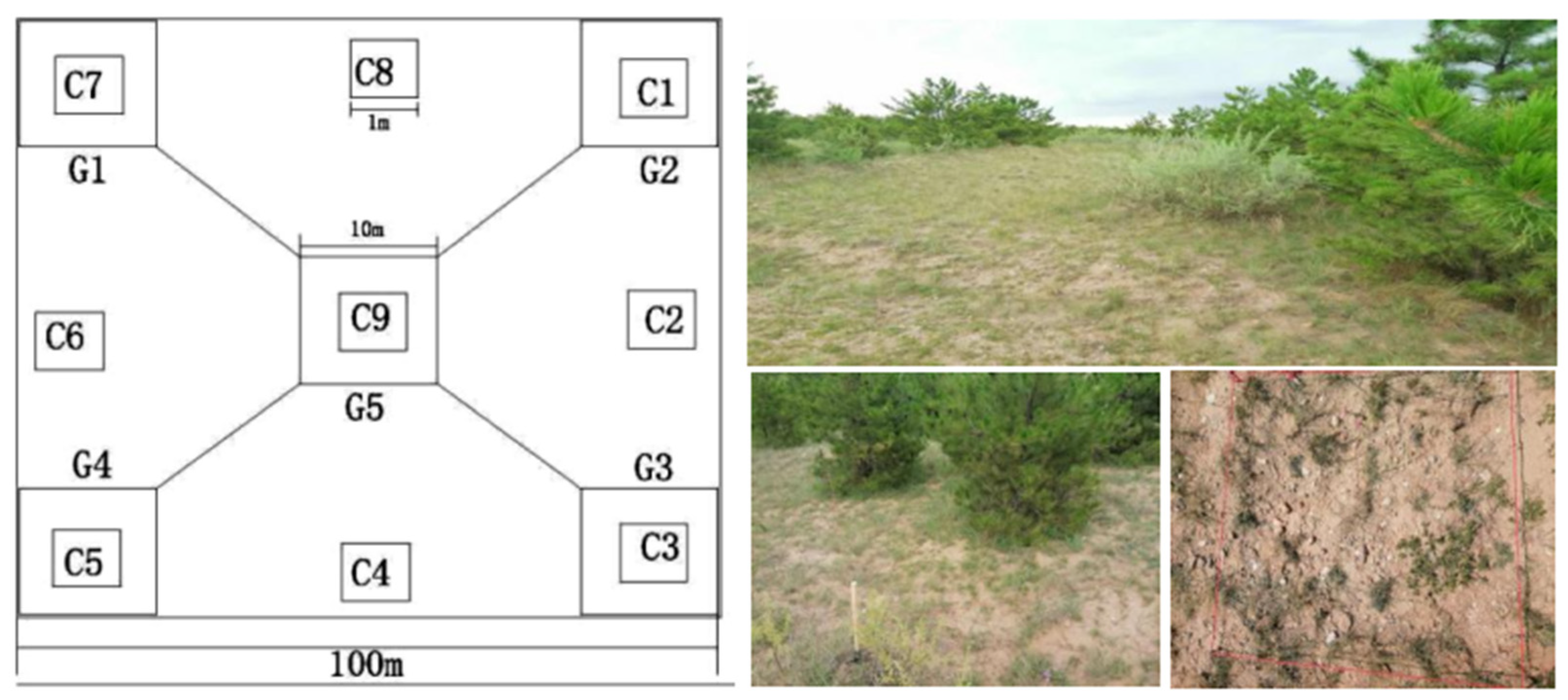
2.2.1. Plot Layout and Vegetation Survey

Eight typical protective areas were selected for the plant community survey between June and August 2020–2022. A survey point with evenly distributed vegetation was selected within each area to ensure that the sampling was representative. A 100 m × 100 m plot was designated at each selected survey point (Figure 2). Using the 5-point quadrat sampling method, 5 20 m × 20 m quadrats and 9 1 m × 1 m herbaceous quadrats were established within each plot [18]. Within the quadrats, information on the arbor and shrub species, the number of stems (density), the diameter at breast height (DBH), the height, and the canopy width were recorded. Additionally, the species and number of dead arbors and shrubs were recorded. The herbaceous quadrats were surveyed to determine the community species composition, density, height, and coverage. Plant height refers to the vertical distance from the highest point of a plant in its natural state to the ground. Canopy width is defined as the product of widths in the north–south and east–west directions of the sapling. The height, growth rate, and canopy width were measured using a steel tape. Ground diameter refers to the diameter of the sapling stem close to the ground, and it was measured using digital calipers [19]. The survey results are shown in

Table 1. Overview of community structure in the eight configuration modes.

Pattern	Altitude/m	Slope/°	Aspect of Slope	Different Slope Position Configuration Structure
				Slope Top	Slope Middle	Slope Bottom
1	1439	15	NW	Grass	arbor + Shrub + Grass	Grass
2	1418	13	NW	arbor + Grass	arbor + Shrub + Grass	Shrub + Grass
3	1416	16	NW	arbor + Grass	Shrub + Grass	arbor + Grass
4	1426	14	NW	arbor + Grass	arbor + Shrub + Grass	arbor + Shrub + Grass
5	1420	14	NW	Grass	Grass	Grass
6	1431	13	NW	Grass	Shrub + Grass	Shrub + Grass
7	1425	15	NW	Shrub + Grass	Grass	Shrub + Grass
8	1427	15	NW	Shrub + Grass	Grass	Grass

Note: all the trees in the plant community in this study were Pinus tabuliformis, and the shrub species were Caragana korshinskii Kom. Both trees and herbs were planted in the 1980s, and the herb species were mainly Stipa spp., Leymus chinensis, and other plants.

.

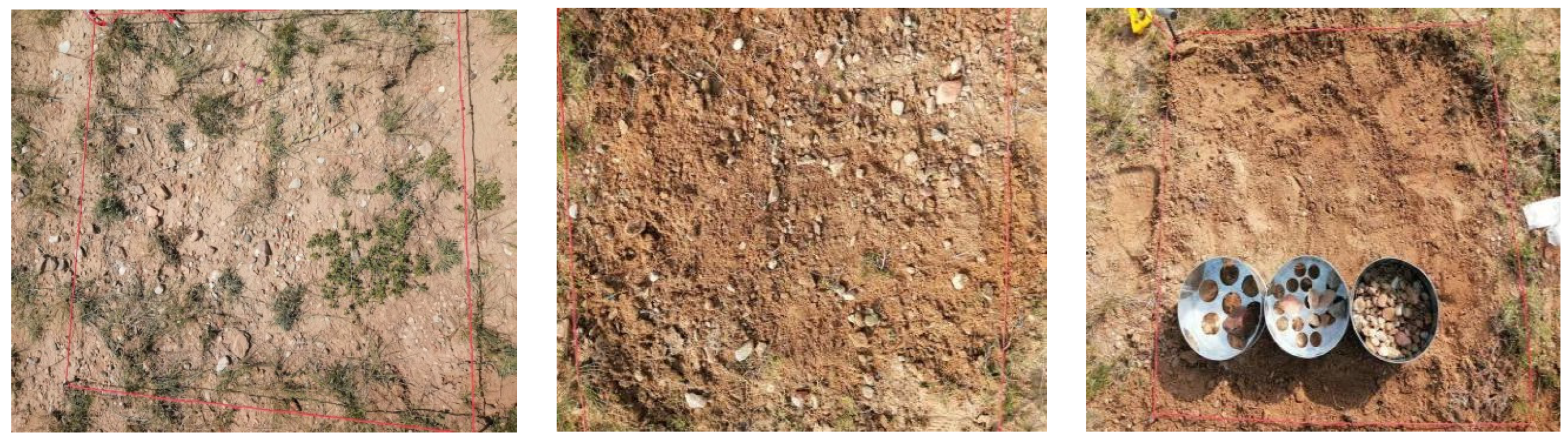
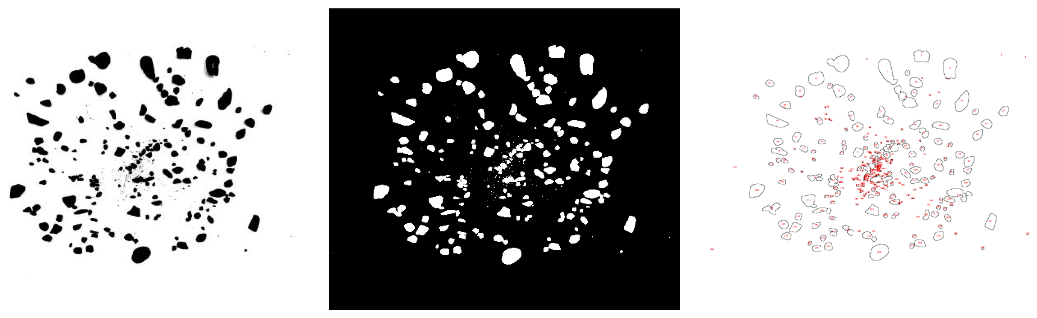
2.2.2. Determination of the Surface Gravel Coverage

Three 1 m × 1 m gravel quadrats were uniformly selected at each sampling point. Surface weeds were removed, and the top 0–5 cm of the soil within the quadrat was collected. After an initial field screening, the gravel retained on each sieve layer was gathered, sorted based on particle size, stored in sealed plastic bags, and labeled for identification (Figure 3).

The collected gravel samples were air-dried in the laboratory. They were then rinsed several times with clean water until all adhering substances were completely removed. Once dried, gravel pieces were stained with ink and air-dried in a cool place for 12 h until they turned completely black. The stained gravel pieces were then randomly scattered on a square wooden board with a white background (side length, 100 cm) [20]. A digital camera was used to capture three sets of photographs of the gravel, which were then stored, labeled, and processed using ImageJ 2018 software to determine the gravel coverage (Figure 4).

2.2.3. M. Godron’s Method for Determining Community Structural Stability

The stability of the plant community structure was assessed using M. Godron’s method of stability determination [21]. First, the measured plant coverage was sorted in descending order and then converted to the relative coverage. Subsequently, these relative coverages were cumulatively added in descending order to calculate the cumulative relative coverage, represented by (y). The inverse of the total herbaceous plant coverage within the plot was calculated and cumulatively summed based on the number of plant species, termed as the species cumulative percentage, represented as (x) [22].

The results were fitted using a curve equation, with the intersection of the straight line (y = 100 − x) and smoothed curve serving as the reference point for plant community stability.

Equation (1):

$${\mathit{RC}}_i=C_i/C_T,$$

(1)

where RC_i is the relative canopy cover of the ith species, C_i is the canopy cover of the ith species, and C_T is the total canopy cover of species in the sample plot.

Equation (2):

$$X={\displaystyle {\sum }_{i=1}^S\frac{1}{S}},$$

(2)

where X is the cumulative percentage of species, i is the ith species, and S is the total number of species.

Equation (3):

$$Y={\displaystyle {\sum }_{i=1}^S{\mathit{RC}}_i},$$

(3)

where Y is the cumulative relative canopy cover, RC_i is the relative canopy cover of the ith species, and S is the total number of species.

The linear equation is

$$Y=100-x,$$

(4)

When the smoothed curve is fitted to the system of linear equations and combined with the linear equation, the resulting value of x should be selected such that both x and Y are real numbers greater than 0 and represent where the curve intersects. The coordinates (x, Y) of this intersection point and the Euclidean distance to the stability point (20, 80) determine the level of stability. A shorter distance from the intersection to the reference point implies a more stable community, whereas a longer distance indicates an unstable community [23].

2.2.4. Investigation of the Water Retention Function of Litterfall

Measurement of Litterfall Water-Holding Capacity

Three 0.5 m × 0.5 m plots were set up diagonally in each sample site. Although the natural state of the litterfall was maintained, the species composition, thickness, and cover of the litterfall within the plot were measured using both the ruler and grid collection methods. After recording the measurements, litterfall was collected from the undecomposed and semi-decomposed layers separately, placed in sealed plastic bags, labeled, and weighed to obtain the fresh weight (Figure 5).

The litterfall samples were dried in a constant-temperature oven (80 °C) until a constant weight was reached. The dry weight per unit area was measured to determine the litterfall accumulation. The water-holding capacity and absorption rate of the litterfall were measured using a fixed-time soaking method. At intervals of 0.08 h (5 min), 0.17 h (10 min), 0.25 h, 1 h, 1.5 h, 2.5 h, 4.5 h, 12 h, and 24 h, the soaked litterfall was removed, left to allow the weight to stabilize, and then weighed to record the water retention process and to calculate the water-holding capacity and absorption rate for each soaking time. The maximum retention capacity of litterfall occurred when the maximum retention capability was reached. However, under actual rainfall, due to the influence of factors such as gravity and the slope, the actual retention amount was only 0.85 times the maximum, known as the effective retention amount. The calculation formulae are as follows [24].

The natural moisture content of litterfall (R₀%):

$$R_0=\frac{\left(W_1-W_2\right)}{W_2}\times 100\%,$$

(5)

where W₁ is the wet weight of the litterfall (g) and W₂ is the dry weight of the litterfall (g).

Dry accumulation of litterfall per unit area:

$$M=\frac{W_2\times {10}^{-6}}{2.5\times {10}^{-5}},$$

(6)

Maximum water-holding rate of the litterfall:

$$R_{\mathit{hmax}}=\frac{W_3-W_2}{W_2}\times 100,$$

(7)

where W₃ is the water content of litter after 24 h immersion in water (g).

Maximum water-holding capacity of litterfall:

$$W_{\mathit{hmax}}=\frac{R_{\mathit{smax}}\times M}{100},$$

(8)

Maximum retention rate of litterfall:

$$R_{\mathit{smax}}=R_{\mathit{hmax}}-R_0,$$

(9)

Maximum retention amount of litterfall:

$$W_{\mathit{smax}}=\frac{R_{\mathit{smax}}\times M}{100},$$

(10)

Effective retention rate of litterfall:

$$R_{\mathit{sv}}=(0.85R_{\mathit{hmax}}-R_0)\times 100,$$

(11)

Effective retention amount of litterfall:

$$W_{\mathit{sv}}=\frac{R_{\mathit{sv}}\times M}{100}$$

(12)

Evaluation of Water Retention Function of Litterfall

This study used a coordinate comprehensive evaluation method to investigate the water retention function of litterfall in P. tabuliformis forests under four different modes [25]. The evaluation criteria were based on the following six indicators (n = 6): thickness of litterfall, maximum water-holding rate, effective retention rate, accumulation amount, maximum water-holding amount, and effective retention amount. First, each indicator is standardized, where i denotes different densities of P. tabuliformis forests and j represents different indicators. The original data are denoted as X_ij, and X_j signifies the maximum value of each indicator. Based on Formula (13), the relative value d matrix coordinates are obtained. Then, according to Formula (14), the distance of the j indicator of the P. tabuliformis forest of density to the standard point is calculated. Finally, based on Formula (15), the sum Si of the distances of each indicator of the P. tabuliformis forest of density i to the standard point can be obtained. A smaller evaluation value indicates a relatively higher water retention function [26].

$$d_{\mathit{ij}}=X_{\mathit{ij}}/X_j,$$

(13)

$$P_{\mathit{ij}}=\sqrt{{\displaystyle \sum _i(1-d_{\mathit{ij}}{)}^2}},$$

(14)

$$\mathit{Si}={\displaystyle \sum _{j=1}^n{P}_{\mathit{ij}}},$$

(15)

2.2.5. Saturated Hydraulic Conductivity of Soil

The saturated hydraulic conductivity refers to the amount of water that flows through a unit area of soil under a unit hydraulic gradient over a unit time when the soil is saturated. A ring knife was used to collect undisturbed soil samples, and a filter paper of the same size as the ring knife was placed with its bottom facing upwards. A piece of gauze was wrapped around the bottom of the ring knife using a rubber band. The gauzed end of the ring knife was immersed in a container filled with standing water until the water level was approximately 1 mm from the top of the ring knife. After the ring knife was saturated, it was weighed. The water content at this point represented the saturated water content of the soil. A saturated weighed ring knife was placed in a funnel with a plastic cup underneath. An empty ring knife was fitted over each saturated ring knife, and the junction was sealed with glue, tape, or rubber bands to ensure that no water leaked. The ring knife was connected to a Mariotte bottle, and the water head was adjusted to approximately 2 cm. Timing began once the water began to infiltrate the ring-knife sample. The infiltration volumes were recorded at intervals of 1, 2, 5, 10, 20, and 30 min. Each interval was measured 10 times until a steady infiltration rate was achieved. The stable infiltration rate was calculated based on the infiltration volume and time [27] using the following formula:

$$K_0=\left(10\mathit{QL}\right)/\mathit{Atn}(H+L),$$

(16)

where K₀ represents the measured saturated hydraulic conductivity of the soil (mm/min), Q is the flow volume of water in the ring knife over the measurement time (cm³), L is the height of the ring knife (5 cm in this study), A is the cross-sectional area of the ring knife (20 cm²), t is the measured time (min), and H is the height of the water head (cm).

The measured values were converted to those at 10 °C using the following formula [28]:

$$K_s=K_0/(0.7+0.03t_0),$$

(17)

where K_s is the saturated hydraulic conductivity of the soil at 10 °C (mm/min) and t₀ is the temperature (°C) at which the saturated hydraulic conductivity of the soil was measured.

2.2.6. Calculation of Species Diversity

Plant diversity serves as a foundational tool for studying the organizational level and functional status of communities, and acts as a prime indicator of the state of soil and water conservation in the research area. The quantitative characteristics of plant communities can be analyzed by surveying and recording the types, canopy coverage, and frequency of plants in the study area [29]. Species diversity indices include the species richness index, Shannon–Wiener diversity index, and Pielou’s evenness index. The diversity index D is calculated based on its importance [30]:

$$\mathit{ImportanceValue}=(\mathit{CR}+\mathit{HR}+\mathit{DR})/3,$$

(18)

where CR is the relative canopy coverage, HR is the relative height, and DR is the relative density.

Relative Density (%) = (number of individuals of a species/total number of species) × 100%

(19)

Relative Canopy Coverage (%) = (Canopy coverage of a species/Total canopy coverage of all species) × 100%

(20)

Relative Height (%) = (Average height of a species/Sum of average heights of all species) × 100%

(21)

Species Richness Index:

$$R=S,$$

(22)

where S represents the number of species in each sample plot.

Shannon–Wiener Diversity Index:

$$D=-{\displaystyle \sum P_i}{\mathit{lnP}}_i,$$

(23)

Pielou’s Evenness Index:

$$J=D/\mathit{lnS}$$

(24)

where P_i = N_i/N, N_i is the importance value of the i species, and N is the sum of the importance values of all species in the community.

2.2.7. Data Processing

Data were summarized and statistical analyses were performed using Excel software 2020. Vegetation canopy cover and diversity indices were calculated. The M. Godron community structure stability graph was plotted using Origin 2021 software. The surface gravel coverage was computed after scanning with ImageJ software. Schematic diagrams of the plant layout were generated using Figdraw 2019 software. The research process is shown in Figure 6.

3. Results and Analysis

3.1. Characteristics of Plant Communities in the Study Area

Analysis of Plant Diversity Indices under Different Configuration Modes

Plant diversity is a vital indicator of ecosystem stability that plays a pivotal role in preventing soil erosion, sustaining soil productivity, and other aspects [31]. Indices such as the Margalef richness index, Simpson index, and Pielou evenness index can directly reflect the stability of ecosystems and have been widely applied in the field of ecology.

From Figure 7, a comprehensive analysis incorporating the Margalef richness index, Simpson index, Pielou evenness index, and Shannon–Wiener index revealed that plant diversity varied under different configuration modes. At the slope top and middle, the species diversity in the arbor + grass and arbor + shrub + grass configurations was higher than in the shrub + grass and pure natural herb configurations. Thus, in the hilly slope tops and middle areas, the arbor + grass and arbor + shrub + grass composite configurations dominated. However, species diversity at the slope base was not significantly affected by forest structure. Studies have shown that soil from the top and middle of a slope erodes and accumulates at the slope base, resulting in a thicker soil layer. In hilly areas, soil influences plant growth more than forest structure, leading to a lack of significant differences in species diversity at the slope base among the various configuration modes.

Considering species diversity, four arbor + shrub + grass configuration types that exhibited higher diversity among the existing eight protective modes were selected for comparative analysis. For different slope positions, the soil and water conservation performances were assessed based on different evaluation indices. The best protective mode for soil and water conservation in hilly areas was established based on the excellence of these indices. The simulation diagrams of the four selected protective modes shown in Figure 8 are based on field investigations.

For detailed investigation, the slope was divided into three parts based on the forestry classification standards for slopes: the top, the middle, and the bottom. The specific configuration modes are presented in

Table 2. Plant configurations of the four protective modes.

Pattern	Position	Species of Arbors	Configuration Structure (Plant Space × Row Space)	Quantity (Strain/hm2)
P-1	Slope top	Herbal	——	——
	Slope middle	P. tabuliformis Caragana korshinskii	5 m × 6 m 6 m × 1 m	333 1667
	Slope bottom	Herbal	——	——
P-2	Slope top	C. korshinskii	1 m × 5 m	2000
	Slope middle	P. tabuliformis C. korshinskii	5 m × 3 m 1 m × 5 m	667 2000
	Slope bottom	C. korshinskii	1 m × 5 m	2000
P-3	Slope top	P. tabuliformis	3 m × 3 m	1111
	Slope middle	C. korshinskii	1 m × 3 m	3333
	Slope bottom	P. tabuliformis	3 m × 3 m	1111
P-4	Slope top	P. tabuliformis	5 m × 5 m	400
	Slope middle	P. tabuliformis C. korshinskii	5 m × 10 m 1 m × 10 m	200 1000
	Slope bottom	P. tabuliformis C. korshinskii	5 m × 5 m 1 m × 5 m	400 2000

Note: P-(1–4) represent different configuration modes.

.

3.2. Protective Forest Configuration Effects at the Slope Top

3.2.1. Analysis of Surface Gravel Coverage under the Canopy

The goal of slope treatment is to reduce the runoff time and intensity on the slope surface to prevent soil erosion. As the highest part of the mountain, the slope top has infertile soil and high gravel coverage. This makes the slope top highly susceptible to wind and water erosion, leading to substantial nutrient loss. Therefore, the treatment of the top slope is of paramount importance [32].

The primary protective modes at the top of the study area were natural grass recovery, shrub–grass protection, arbor–shrub–grass protection, and arbor–grass protection. To compare the effects of different configuration modes, ImageJ software was used to analyze the characteristics of the exposed surface gravel at the top of the slope (Figure 4). Based on gravel particle size classification standards, the gravel particle size ranged from 1 cm to 8.4 cm. In this study, gravel particles of size D were categorized into the following three size ranges for analysis: 1–3 cm, 3–5 cm, and >5 cm.

As shown in Figure 9, there were significant differences in the surface gravel coverage at the top of the slope under the four configuration modes. The percentages of surface gravel coverage per unit area for modes 1–4 were 46.7%, 40.5%, 7.6%, and 6.3%, respectively. The gravel coverage at the slope top without vegetation measures and under pure shrub configurations was similar, and significantly higher than that under pure arbor forests and arbor–shrub mixed forests at six to seven times their coverage.

The size of the exposed gravel at the top of the slope was further analyzed using sieving and measuring methods. As shown in Figure 10, different protective modes influenced surface gravel of different sizes to varying extents. For gravel sizes in the ranges of 1 cm < D < 3 cm and 3 cm < D < 5 cm, the surface gravel coverage under the bare land and pure shrub modes was significantly higher than that under the pure arbor and arbor–shrub modes. However, this difference was not pronounced for D > 5 cm. In this study, it was observed that smaller gravel particles were mainly composed of arsenopyrite, which quickly dissolves upon contact with water, supplying the flow with substantial sandy material. Given that the slope top is the highest point of the mountain, providing ample force for water flow directly leads to mudslides, posing a significant threat to local ecological safety. Hence, arbor–grass or arbor–shrub–grass configurations should be applied for protection at the slope top, essentially opting for Mode 3 or Mode 4 to effectively reduce the amount of soil carried away by water erosion and minimize soil and water losses. This approach is termed the “cap on the mountaintop” strategy.

3.2.2. Comparison of Growth Conditions between the Two Configuration Modes

The cap on the mountaintop configuration mode had a noticeable effect on intercepting flow and reducing sediment on the slope top. However, in practical applications, it is crucial to focus on the survival and growth conditions of the protective forests. The survival rate and growth directly affect the ecological benefits of forests. Hence, the ecological methodology of “three dimensions, one quantity” was used to compare the growth index characteristics of the arbor layer at the slope top for Mode 3 and Mode 4 to identify the optimal configuration mode for slope top protection.

The most significant difference between the two modes was in the spacing between arbor plants. In Mode 3, the plant spacing was 5 m × 5 m, whereas in Mode 4, it was 3 m × 3 m. As shown in Figure 11, after comparing the growth indices of the arbor layers for the two configurations, it was observed that the average height, average DBH, and average timber volume of the Mode 3 arbor layer were all higher than those of Mode 4. The average coverage per unit area was similar in both groups. A comprehensive comparison indicated that Mode 3 was superior to Mode 4. The main reason for this is that in Mode 4, the interplant distance is shorter. Although this initially leads to a denser forest canopy, as time progresses, the adverse effects of excessive planting density become more evident. This is mainly reflected in greater competition between species, which results in slower plant growth. The overall development and stability of such forests deteriorate over time, increasing their susceptibility to pests and diseases. This can cause the death of many plants. Therefore, when the arbor plant spacing at the top of the slope was 5 m × 5 m, this spacing offered the best long-term protective effect for the slope top.

3.3. Protective Forest Configuration Mode Effect on the Slope Middle

3.3.1. Analysis of Forest Stand Community Structural Stability

The mid-slope area is crucial for maintaining slope stability. This area effectively slows slope runoff erosion and reduces the chances of flash floods, making it a primary protective area in hilly regions. This study adopted the modified M. Godron stability measurement method and employed Origin 2021 software to simulate the curves for the four slope-protection modes (Figure 12). According to the principle of M. Godron stability and the intersection coordinates of the smooth curve and the straight line, the closer the intersection coordinate values are to the equilibrium point (20, 80), the more stable the community structure [33]. The Euclidean squared distance between the intersection and equilibrium points was used as the evaluation standard to intuitively express the difference in distance between the intersection and equilibrium coordinates. The smaller the distance, the greater the stability. The results are presented in

Table 3. Impact of different configuration modes on plant community stability.

Pattern	Fit Line	R2	Intersection Coordinates	Euclidean Square Distance	Judgment Results
P-1	y = −0.0055x2 + 0.9421x − 58.8068	0.97	(22.65, 77.35)	14.05	Stabilize
P-2	y = −0.00943x2 + 1.3931x − 50.5464	0.93	(22.69, 77.31)	14.52	Stabilize
P-3	y = −0.00922x2 + 1.3884x − 49.7916	0.94	(24.08, 75.92)	25.94	Instabilize
P-4	y = −0.0102x2 + 1.5875x − 40.7730	0.99	(25.44, 74.56)	59.21	Instability

.

From Figure 13 and Table 3, the results of the community structure stability assessment for the four configuration modes are as follows:

The Mode 1 community stability fitting equation is y = −0.0055x² + 0.9421x − 58.8068, with intersection coordinates at (22.65, 77.35) and a Euclidean squared distance of 14.05 from the equilibrium point. Among the four modes, this distance was the smallest.

The Mode 2 vegetation community stability fitting equation is y = −0.00943x² + 1.3931x − 50.5464, with intersection coordinates at (22.69, 77.31) and a Euclidean squared distance of 14.52 from the equilibrium point. This distance was slightly less than that of Mode 1. However, the difference between the two modes was not significant, and the vegetation community stability was similar.

The Mode 3 vegetation community stability fitting equation is y = −0.00922x² + 1.3884x − 49.7916, with intersection coordinates at (24.08, 75.92) and a Euclidean squared distance of 25.94 from the equilibrium point, which was higher than in Mode 1 and Mode 2.

The Mode 4 community stability fitting equation is y = −0.0102x² + 1.5875x − 40.7730, with intersection coordinates at (25.44, 74.56) and a Euclidean squared distance of 59.21 from the equilibrium point. This was significantly higher than that of the first three modes. The main reason was that the Mode 4 mid-slope configuration of the P. tabuliformis forest had a spacing of 3 m × 3 m, resulting in a larger canopy closure per unit area. This limited the photosynthesis of plants underneath, leading to poor growth conditions. As a result, the vegetation community stability was the worst. In Mode 3, the spacing between arbor species was larger, leading to weaker soil and water conservation effects as well as soil erosion, which caused the loss of nutrients necessary for plant growth.

In general, an appropriate configuration mode is the key factor for maximizing the soil and water conservation role of a forest stand, minimizing soil nutrient loss, benefiting vegetation growth and recovery, and playing a decisive role in the stability of the plant community.

3.3.2. Hydrological Benefits of Understory Litter under Different Configuration Modes

The litter layer, which acts as the second functional layer in forests for water conservation, possesses robust runoff interception and water-retention properties. Its water retention capacity is two to five times its dry weight and plays an extremely vital role in the hydrological processes of the forest ecosystem [34].

As shown in Figure 13, a comprehensive comparison of six indicators (the litter thickness, accumulation, maximum water retention rate, effective water retention volume, effective interception rate, and effective interception volume under different configuration modes) revealed that the accumulation of the semi-decomposed litter layer was two to four times that of the undecomposed layer, and its thickness was doubled. The water retention and interception rates of the semi-decomposed layer were also higher, indicating their key roles in water conservation. Among the four configuration modes, the indicators of litter thickness, accumulation, water retention, and interception rate in Mode 1 were significantly higher than those in the other three modes, suggesting that the water conservation function of understory litter in P-1 was superior to that in the other three modes.

Analyzing the water retention capability indicators of understory litter under different configuration modes revealed varying patterns, making it challenging to evaluate the water conservation function of litter under different modes. The comprehensive coordinated evaluation method adopted in this study can address this issue effectively.

The results of the evaluation of the water conservation function of understory litter under the four configuration modes are shown in

Table 4. Evaluation of water conservation function of P. tabuliformis litter at different densities in Ziwuling, Loess Plateau.

Pattern	Thickness	Max. Water Retention	Effective Retention Rate	Standing Volume	Max. Water Capacity	Effective Storage Capacity	Evaluate	Sort
P-1	0.00	0.02	0.14	0.00	0.00	0.00	0.16	1
P-2	0.17	0.00	0.00	0.33	0.25	0.07	0.82	2
P-3	0.25	0.02	0.01	0.28	0.35	0.25	1.16	3
P-4	0.21	0.15	0.14	0.23	0.21	0.17	1.11	4·

. The understory litter water conservation function in Mode 1 was significantly better than those of the other modes. Therefore, based on a comparative analysis of the stability of the plant community structure and the water conservation function of litter under different configuration modes, it is recommended that a protection mode of arbors + shrubs + herbs be adopted in the mid-slope area during actual slope protection processes. In this mode, the arbor stand spacing should be 5 m × 6 m, the understory Caragana korshinskii spacing should be 1 m × 6 m, and the herbaceous layer should primarily consist of naturally regenerated plants.

3.4. Protective Effect of Slope Bottom Configuration Modes

3.4.1. Analysis of Ks

The Ks refers to the flow rate of water through a fixed area of soil when the soil is saturated and under a unit hydraulic gradient [28]. The Ks, as an essential indicator of soil permeability, is conducive to the infiltration of rainfall into the soil, reducing surface runoff and thereby achieving the objectives of disaster mitigation and water conservation. In the slope bottom areas, where the soil layer is relatively thick, a higher Ks can effectively slow the flow of water, thus reducing soil and water erosion.

As shown in Figure 14, research on the saturated hydraulic conductivity of the 0–60 cm soil layer under the 4 slope bottom vegetation configuration modes revealed the following:

For the 0–20 cm soil layer, the Ks ranged from 0.17 to 3.87 mm/min, with an average Ks of 1.38–1.47 mm/min. For the 20–40 cm soil layer, the Ks ranged from 0.43 to 1.73 mm/min, with an average Ks of 0.74–0.79 mm/min. For the 40–60 cm soil layer, the Ks ranged from 0.23 to 0.69 mm/min, with an average Ks of 0.42–0.45 mm/min.

Overall, the trend revealed higher values in the topsoil that gradually decreased with depth. This pattern corresponded to the changes in the saturated hydraulic conductivity values along the soil profile. However, no significant differences were observed in the average saturated hydraulic conductivity of the soil within the same soil layer. This phenomenon was primarily influenced by the soil texture. The soil in the study area consists mainly of antimony shale, which dissolves upon contact with water. The distribution characteristics of the arbors and shrub roots also affected the saturated hydraulic conductivity. During the research, it was found that within a 0–50 cm radius under the arbor or shrub canopy, the Ks was relatively high. When the radius exceeded 50 cm, the conductivity gradually decreased. This phenomenon was mainly due to the fact that the herbaceous cover beneath the arbor canopy at the slope bottom was less than that without arbors. Therefore, although arbors and shrubs increased the Ks within a certain range, there was no difference in the average conductivity when calculated over the entire plot. This was also a significant factor contributing to the observed variability in the Ks within the same configuration mode (Figure 15).

3.4.2. Variation Coefficient of Ks

In classical statistics, the coefficient of variation (Cv) is used to analyze the variability characteristics. Based on the degree of variation, a Cv of ≤0.1 indicates weak variability, 0.1 < Cv ≤ 1 indicates moderate variability, and Cv > 1 signifies strong variability [35].

As shown in Figure 16, significant differences were observed in the Cv for saturated hydraulic conductivity across different soil layers. Overall, the variation was moderate. Ranked in order of the Cv magnitude, the sequence was arbor + shrub + grass mode > arbor + grass mode > shrub + grass mode > pure herbaceous mode. This indicates that the more complex the vegetation configuration mode, the greater the Cv for the Ks.

Considering both the average Ks per unit area and the Cv and adhering to the principles of scientific protection and cost efficiency, the protective mode at the slope bottom should mainly consist of naturally recovered herbaceous plants, supplemented with artificial maintenance and grazing prohibition measures to ensure the stable growth of the herbaceous community.

4. Discussion

4.1. Diversity of Different Forest Stand Structures

Species diversity is fundamental for the functioning and maintenance of ecological systems. Most forests experience varying degrees of human activity. Plant paracommunities are influenced by fragmentation and climate change, leading to the formation of microhabitats within these regions [36]. There is limited understanding of how environmental heterogeneity affects community composition, structure, and function. Environmental heterogeneity is a crucial factor in the development of biodiversity conservation plans [37]. Different forest types have different species compositions, resulting in distinct structures. Secondary forests exhibit structures formed through long-term interactions between forest plants and the environment. In contrast, plantations often display inferior spatial structures because of their regeneration methods. Species diversity determines the complexity of community structure and function, reflecting multifaceted differences in the community [38].

Vegetation restoration directly manifests itself as the recovery of plant diversity. Studies of plant diversity beneath various forest stand structures have revealed significant differences in the Shannon–Weiner diversity index, Simpson diversity index, and Pielou’s evenness within the herbaceous layer among different stand structures. Species diversity and dominance in the arbor + shrub + grass mode were markedly higher than in the shrub + grass and sole herbaceous modes. The arbor + shrub + grass mode exhibited the most uniform distribution with the highest species diversity and richness. This indicates that compound structural stands can effectively enhance plant diversity in hilly and gully areas, thereby improving the regional environment [39]. However, when the spacing between arbors was too small, the richness of the interspecies plants significantly diminished. Although such communities approach climax communities and become almost entirely closed canopies, the growth and renewal capabilities of understory plants decline. Consequently, the herbaceous layer has diminished species richness and shows a notable lack of resilience and adaptability to environmental change. Density plays a significant role in seedling survival rates and the maintenance of species diversity. Competition for resources such as sunlight and soil nutrients also affects the persistence of species diversity [40].

4.2. Community Structure Stability

4.2.1. Relationship between Plant Diversity and Community Structure Stability

Community stability refers to the ability of a community to maintain interspecies interactions and achieve relative equilibrium, as well as its capacity to recover to a stable state when subjected to external disturbances [41]. It is commonly believed that the more complex the community structure and the higher its species diversity, the more stable the community. Thus, community diversity is an essential metric for stability [42]. In this study, the stability of the herbaceous communities beneath various vegetation configurations mirrored the trend in plant diversity. A study by Zhang et al. (2023) [43] found that species diversity can enhance community productivity, optimize ecosystem functions, and bolster community stability. Meanwhile, Keersmaecker et al. (2014) [44] reported on the relationship between biodiversity and ecosystem stability. They posited that plant diversity serves as a critical barrier to sustaining ecosystem functions when plant communities face severe external disturbances. This is an indispensable condition for maintaining community stability. An increase in plant diversity tends to enhance community stability. This aligns with the findings of the present study that when the total community density is held constant, the species density variability diminishes with increased species diversity, subsequently enhancing community stability. However, some researchers have argued that species diversity does not correlate linearly with stability. The driving force behind the stability introduced by species diversity is not the diversity itself, but the community’s ability to include species or functional groups. Gu et al. (2020) [45], in their analysis of community diversity and stability in mining areas, found no significant correlation between the two.

The study area, which is characterized as a hilly gully region, has a fragile environment. The primary vegetation type in natural succession in this area consists of herbaceous plants, and the study area is currently in an early succession stage, with limited plant species and no mature functional groups. In artificial forests, the native species combination of P. tabuliformis and C. korshinskii was found to have the highest species diversity. However, the community stability varied depending on the configuration mode. This finding indicates that community stability is closely associated with multiple factors. The sole use of species diversity to explain community stability has limitations, particularly during the initial phase of community construction. Birmele et al.’s (2015) [46] research suggests that as community succession progresses, the structural units with strong and very strong interspecies combinations increase, the species richness grows, and the forest stability strengthens. Hu et al. (2016) [47] research also indicates that the community succession trend progresses from instability to stability. The aim of this study was to enhance the ecological quality of the mixed P. tabuliformis forest in the study area, including both artificially planted and naturally occurring forest stands. Given its simple arbor species composition and structure, only appropriate configuration methods can increase the community stability. Therefore, selective logging and replanting can be performed in relatively unstable forests to increase the species richness and promote positive succession in artificial forests.

4.2.2. Community Stability Research

The stability of the vegetation community in hilly gully regions presents an intricate issue. To date, there is no unified understanding or methodological framework regarding community stability, its influencing mechanisms, and measurement approaches [48]. Research on community stability is generally based on a linear regression succession. The M. Godron method has been widely adopted for stability measurements. This offers a systematic and comprehensive approach to gauging the stability of vegetation communities. This method, which is based on the overall characteristics of the vegetation community, effectively mirrors the developmental trajectory and evolving trends of the community. Given that the present study focused on the hilly gully region of China, which is characterized by complex geographical features, topography, and soil, among other environmental factors, the M. Godron method was modified. In the revised approach, plant species were substituted for vegetation cover. Combined with mathematical modeling, this made the M. Godron stability measurement method more quantitative, thereby enhancing its credibility. This approach provided a more intuitive representation of the stability of vegetation communities. By eliminating subjective human influence, this approach more accurately represented the stability of vegetation communities, aligning with the principles of ecological development [49].

4.3. Factors Affecting the Water-Holding and Retention Abilities of Litter

The water-holding capacity of litter is a crucial indicator of its ability to retain moisture and its role in water conservation. This can be quantified through metrics such as the maximum water-holding capacity and the maximum water-holding rate. Research by Song et al. (2012) [50] and others on three forest types in the southwestern mountainous region found no significant difference between the maximum water-holding capacities of partially decomposed and undecomposed litter layers. This suggested that the degree of litter decomposition did not significantly influence the maximum water-holding capacity. In contrast, the present study found that the maximum water-holding capacity of partially decomposed litter was significantly higher than that of undecomposed litter. This could be because litter storage in different forest types was positively correlated with the maximum water-holding capacity, and there was no significant difference in litter storage among the different decomposition layers, making the difference in their maximum water-holding capacities insignificant.

The effective retention volume and rate of litter are estimates of how litter intercepts rainfall, factoring in its natural moisture content, and reflecting the actual water conservation function of the litter. Liu et al. (2016) [13] study on the typical forest litter storage and water-holding ability in the southwestern mountain region found that there were no significant differences in the effective retention volume and rate between different forest types, whether in the partially decomposed or undecomposed litter layers. Moreover, the maximum water-holding capacity and effective retention volume of litter under different forest configurations were positively correlated. However, the magnitude of the correlation showed no evident patterns across different forest types or decomposition layers. Conversely, Hu et al. (2021) [15] study of the litter of seven artificial forests in the plains and lake region of the middle Yangtze River found that the effective retention volume of the partially decomposed layer was higher than that of the undecomposed layer, whereas the effective retention rate of the undecomposed layer surpassed that of the partially decomposed layer. However, the present study observed that both the effective retention volume and rate were higher in partially decomposed litter than in the undecomposed layer. These discrepancies might arise from the insignificant differences in litter storage among the decomposition layers and the litter’s natural moisture content, where the high spatiotemporal variability of the natural moisture content significantly affects its retention rates.

4.4. Factors Influencing the Ks

Existing studies have shown that the factors affecting the Ks vary across different research areas. Furthermore, the interactions between various basic soil properties add to the complexity, resulting in distinct mechanisms affecting the Ks across different regions. The present study revealed that on average, the Ks decreased vertically downward, with the highest values appearing in the topsoil. This phenomenon is primarily due to gravel components in the surface layer and the extensive distribution of plant roots, which leads to higher soil porosity and improved soil water infiltration properties. There was significant variance in the Ks Cv across different plant configurations in the study area, with more complex plant community structures leading to larger variances. Research by Yao et al. (2022) [51] on the Ks of erosion-prone areas in the Loess Plateau showed that the Ks varied to a low degree. Research by Cao (2011) [52] indicated that the Ks of different sandy soils in the Horqin region also had low variability. This suggests that compared with other regions, hill and gully areas exhibit greater variability in terms of the Ks, which is primarily related to sampling locations. The Ks values in the present study were higher closer to arbors or shrubs and lower otherwise.

Of course, many factors affect the Ks. Horn et al. (2020) [53] found that grasslands subjected to heavy trampling exhibited higher variability in topsoil Ks than those not subjected to trampling. The development of root systems in different vegetation types also uniquely affects the soil porosity and bulk density. In a study on the soils of various subtropical vegetation types by Hao et al. (2019) [54], the vegetation type was found to be a crucial factor affecting the Ks. This was mainly because of the varied effects of different vegetation roots on soil porosity and the improvement of water-stable aggregates. In addition, differences in the composition and decomposition states of litter from different vegetation types can change the soil organic matter content to varying extents. As indicated by Gao et al.’s (2023) [55] research, there is a continuous increase in the Ks with the succession of plant communities from grasslands to shrubs and then to forests. Arbors provided the best effects in improving the soil Ks, a conclusion consistent with the findings of the present study. Shi et al. (2023) [56] focused on the Loess Plateau area and analyzed 12 types of vegetation cover, concluding that variations in factors such as the soil litter biomass, capillary porosity, and soil bulk density all significantly influence the Ks. Wang et al. (2023) [57] study on the hydrophysical properties of soils from five land-use types in the Luoyugou basin elaborated on the interrelationships of various factors, revealing significant differences in the Ks across different vegetation types. Evidently, different types of vegetation cover significantly impact soil infiltration abilities, which is in line with the present research findings.

5. Conclusions

In practical work, the primary goal of soil and water conservation is to maximize the ecological functions of vegetation. This study integrated soil hydrological characteristics, plant community structural stability, and litter water-retention capabilities. After analyzing various indicators, including the species diversity in forest structures with different slope positions, the surface gravel coverage, the community structure stability, and the Ks, it was found that composite forest structures with appropriate permeability could effectively enhance species diversity, favoring the stable development of plant communities. The top of the slope, which is the highest point on the mountain, is crucial for soil erosion and is a key area for protection. The capping the mountaintop approach should therefore be adopted. Thus, for the top slope regions, an arbor + grass configuration is recommended, with an arbor spacing of 5 m × 5 m. At this spacing, the surface gravel exposure was minimal, and all arbor species showed optimal growth in the present study. For mid-slope regions, an arbor + shrub + grass structure is recommended, with an arbor spacing of 5 m × 6 m and an underbrush shrub spacing of 1 m × 6 m. In this configuration, the plant community structure was the most stable and the water-retention capability of the underbrush litter was optimal. Further research on the average saturation rate in the lower slope soil revealed that there was no difference in the Ks per unit area between the different configurations. Therefore, the natural restoration of herbaceous plants is suitable for the bottom slope, complemented by conservation measures to prevent disturbances and damage caused by human activities.

References

1. Grima, N.; Edwards, D.; Edwards, F.; Petley, D.; Fisher, B. Landslides in the Andes: Forests can provide cost-effective landslide regulation services. Sci. Total. Environ. 2020, 745, 141128. [Google Scholar] [CrossRef] [PubMed]
2. Li, Y.; Tao, J.; Wu, G.H. Analysis of Ecological Slope Protection Technology in River Regulation. In Proceedings of the 2019 International Conference on Management, Finance and Social Sciences Research (MFSSR 2019), Lyon, France, 2–4 August 2019; pp. 19–22. [Google Scholar] [CrossRef]
3. Zhai, J.; Wang, L.; Liu, Y.; Wang, C. Assessing the effects of China’s Three-North Shelter Forest Program over 40 years. Sci. Total Environ. 2022, 857, 159354. [Google Scholar] [CrossRef]
4. Gyssels, G.; Poesen, J. The importance of plant root characteristics in controlling concentrated flow erosion rates. Earth Surf. Process. Landf. 2003, 28, 371–384. [Google Scholar] [CrossRef]
5. Rey, F. Effectiveness of vegetation barriers for marly sediment trapping. Earth Surf. Process. Landf. 2004, 29, 1161–1169. [Google Scholar] [CrossRef]
6. Wang, Y.; Shangguan, Z. Formation mechanisms and remediation techniques for low-efficiency artificial shelter forests on the Chinese Loess Plateau. J. Arid. Land 2022, 14, 837–848. [Google Scholar] [CrossRef]
7. Wang, S.; Fu, B.; Gao, G.; Liu, Y.; Zhou, J. Responses of soil moisture in different land cover types to rainfall events in a re-vegetation catchment area of the Loess Plateau, China. CATENA 2013, 101, 122–128. [Google Scholar] [CrossRef]
8. Feng, X.M.; Wang, Y.F.; Chen, L.D.; Fu, B.; Bai, G. Modeling soil erosion and its response to land-use change in hilly catchments of the Chinese Loess Plateau. Geomorphology 2010, 118, 239–248. [Google Scholar] [CrossRef]
9. Peng, T.; Wang, S.J. Effects of land use, land cover and soil loss on karts slopes in southwest China. and rainfall regimes on the surface runoff. CATENA 2012, 90, 53–62. [Google Scholar] [CrossRef]
10. Wei, W.; Chen, L.; Fu, B.; Huang, Z.; Wu, D.; Gui, L. The effect of land uses andrainfall regimes on runoff and soil erosion in the semi-arid loess hilly area, China. J. Hydrol. 2007, 335, 247–258. [Google Scholar] [CrossRef]
11. Andres, P.; Jorba, M. Mitigation strategies in some motorway embankments (Catalonia, Spain). Restor. Ecol. 2000, 8, 268–275. [Google Scholar] [CrossRef]
12. Yang, F.; Zhou, Y. Quantifying spatial scale of positive and negative terrains pattern at watershed-scale: Case in soil and water conservation region on Loess Plateau. J. Mt. Sci. 2017, 14, 1642–1654. [Google Scholar] [CrossRef]
13. Li, L.; Li, X.-Y.; Zhang, S.-Y.; Jiang, Z.-Y.; Zheng, X.-R.; Hu, X.; Huang, Y.-M. Stemflow and its controlling factors in the subshrub Artemisia ordosica during two contrasting growth stages in the Mu Us sandy land of northern China. Hydrol. Res. 2016, 47, 409–418. [Google Scholar] [CrossRef]
14. Shen, E.; Liu, G.; Xia, X.; Dan, C.; Zheng, F.; Zhang, Q.; Zhang, Y.; Guo, Z. Resistance to sheet flow induced by raindrop impact on rough surfaces. CATENA 2023, 231, 5514. [Google Scholar] [CrossRef]
15. Hu, Y.; Li, H.; Wu, D.; Chen, W.; Zhao, X.; Hou, M.; Li, A.; Zhu, Y. LAI-indicated vegetation dynamic in ecologically fragile region: A case study in the Three-North Shelter Forest program region of China. Ecol. Indic. 2021, 120, 106932. [Google Scholar] [CrossRef]
16. Wen, B.; Duan, G.; Lu, J.; Zhou, R.; Ren, H.; Wen, Z. Response relationship between vegetation structure and runoff-sediment yield in the hilly and gully area of the Loess Plateau, China. CATENA 2023, 227, 107107. [Google Scholar] [CrossRef]
17. Chen, Z.; Guo, M.; Wang, W.; Wang, W.; Feng, L. Response of soil erodibility of permanent gully heads to revegetation along a vegetation zone gradient in the loess-table and gully region of the Chinese Loess Plateau. Sci. Total. Environ. 2023, 892, 164833. [Google Scholar] [CrossRef] [PubMed]
18. Lu, J.; Feng, S.; Wang, S.; Zhang, B.; Ning, Z.; Wang, R.; Chen, X.; Yu, L.; Zhao, H.; Lan, D.; et al. Patterns and driving mechanism of soil organic carbon, nitrogen, and phosphorus stoichiometry across northern China’s desert-grassland transition zone. CATENA 2023, 220, 106695. [Google Scholar] [CrossRef]
19. Lu, J.; Zhao, X.; Wang, S.; Feng, S.; Ning, Z.; Wang, R.; Chen, X.; Zhao, H.; Chen, M. Untangling the influence of abiotic and biotic factors on leaf C, N, and P stoichiometry along a desert-grassland transition zone in northern China. Sci. Total. Environ. 2023, 884, 163902. [Google Scholar] [CrossRef]
20. Katra, I.; Lavee, H.; Sarah, P. The effect of rock fragment size and position on topsoil moisture on arid and semr arid hillslopes. CATENA 2008, 72, 49–55. [Google Scholar] [CrossRef]
21. Yang, Z.; van Ruijven, J.; Du, G. The effects of long-term fertilization on the teporal stability ofalpine meadow communities. Plant Soil 2011, 345, 315–324. [Google Scholar] [CrossRef]
22. Xie, P.; Liu, T.; Chen, H.; Su, Z. Community Structure and Soil Mineral Concentration in Relation to Plant Invasion in a Subtropical Urban and Rural Ecotone. Forests 2021, 12, 185. [Google Scholar] [CrossRef]
23. Lamit, L.J.; Wojtowicz, T.; Kovacs, Z.; Wooley, S.C.; Zinkgraf, M.; Whitham, T.G.; Lindroth, R.L.; Gehring, C.A. Hybridization among foundation tree species influences the structure of associated understory plant communities. Botany 2011, 89, 165–174. [Google Scholar] [CrossRef]
24. Wong, N.K.; Morgan, J.W. Experimental changes in disturbance type do not induce short-term shifts in plant community structure in three semi-arid grasslands of the Victorian Riverine Plain managed for nature conservation. Ecol. Manag. Restor. 2012, 13, 175–182. [Google Scholar] [CrossRef]
25. Fu, T.; Chen, H.; Zhang, W.; Nie, Y.; Wang, K. Vertical distribution of soil saturated hydraulic conductivity and its influencing factors in a small karst catchment in Southwest China. Environ. Monit. Assess. 2015, 187, 92. [Google Scholar] [CrossRef]
26. Pereira, L.C.; Balbinot, L.; Lima, M.T.; Bramorski, J.; Tonello, K.C. Aspects of forest restoration and hydrology: The hydrological function of litter. J. For. Res. 2021, 33, 543–552. [Google Scholar] [CrossRef]
27. Morbidelli, R.; Saltalippi, C.; Flammini, A.; Cifrodelli, M.; Picciafuoco, T.; Corradini, C.; Govindaraju, R. In situ measurements of soil saturated hydraulic conductivity: Assessment of reliability through rainfall–runoff experiments. Hydrol. Process. 2017, 31, 3084–3094. [Google Scholar] [CrossRef]
28. Aşkın, T. Soil Saturated Hydraulic Conductivity: A Study on Path Analysis in Clayey Soils. Res. Agric. Sci. 2005, 36, 23–25. [Google Scholar]
29. Chand, H.; Verma, K.S.; Bhardwaj, S.K.; Reddy, M.C. Assessment of floral diversity in north western Himalayas—A case study from Kol Dam watershed. Ecol. Environ. Conserv. 2014, 20, 823–828. [Google Scholar]
30. Chen, Y.; Cao, Y. Response of tree regeneration and understory plant species diversity to stand density in mature Pinus tabulaeformis plantations in the hilly area of the Loess Plateau, China. Ecol. Eng. 2014, 73, 238–245. [Google Scholar] [CrossRef]
31. Steur, G.; Verburg, R.W.; Wassen, M.J.; Teunissen, P.A.; Verweij, P.A. Exploring relationships between abundance of non-timber forest product species and tropical forest plant diversity. Ecol. Indic. 2020, 121, 107202. [Google Scholar] [CrossRef]
32. Zhang, X.; Hu, X.; Li, G.; Zhu, H.; Mao, X.; Yuan, X. Time effect of young shrub roots on slope protection of loess area in Northeast Qinghai-Tibetan plateau. Editor. Off. Trans. Chin. Soc. Agric. Eng. 2012, 55, 136–141. [Google Scholar]
33. Hao, G.; Yang, N.; Dong, K.; Xu, Y.; Ding, X.; Shi, X.; Chen, L.; Wang, J.; Zhao, N.; Gao, Y. Shrub-encroached grassland as an alternative stable state in semiarid steppe regions: Evidence from community stability and assembly. Land Degrad. Dev. 2021, 32, 3142–3153. [Google Scholar] [CrossRef]
34. Celentano, D.; Zahawi, R.A.; Finegan, B.; Casanoves, F.; Ostertag, R.; Cole, R.J.; Holl, K.D. Tropical forest restoration in Costa Rica: The effect of several strategies on litter production, accumulation and decomposition. Rev. Biol. Trop. 2011, 59, 1323–1336. [Google Scholar]
35. Zuo, Y.; He, K. Evaluation and Development of Pedo-Transfer Functions for Predicting Soil Saturated Hydraulic Conductivity in the Alpine Frigid Hilly Region of Qinghai Province. Agronomy 2021, 11, 1581. [Google Scholar] [CrossRef]
36. Wan, H.; Bai, Y.; Schönbach, P.; Gierus, M.; Taube, F. Effects of grazing management system on plant community structure and functioning in a semiarid steppe: Scaling from species to community. Plant Soil 2011, 340, 215–226. [Google Scholar] [CrossRef]
37. Faith, D.P.; Walker, P.A. The role of trade-offs in biodiversity conservation planning: Linking local management, regional planning and global conservation efforts. J. Biosci. 2002, 27, 393–407. [Google Scholar] [CrossRef] [PubMed]
38. Alemayhu, A. Role of Participatory Forest Management in Woody Species Diversity and Forest Conservation: The Case of Gimbo Woreda in Keffa Zone South West Ethiopia. J. Environ. Earth Sci. 2019, 9, 1–12. [Google Scholar]
39. Zhang, W.; Huang, D.; Wang, R.; Liu, J.; Du, N. Altitudinal Patterns of Species Diversity and Phylogenetic Diversity across Temperate Mountain Forests of Northern China. PLoS ONE 2016, 11, e0159995. [Google Scholar] [CrossRef]
40. Van Do, T.; Kozan, O.; Tuan, T.M. Altitudinal Changes in Species Diversity and Stand Structure of Tropical Forest, Vietnam. Annu. Res. Rev. Biol. 2014, 6, 156–165. [Google Scholar] [CrossRef]
41. Zelikova, T.J.; Blumenthal, D.M.; Williams, D.G.; Souza, L.; LeCain, D.R.; Morgan, J.; Pendall, E. Long-term exposure to elevated CO2 enhances plant community stability by suppressing dominant plant species in a mixed-grass prairie. Proc. Natl. Acad. Sci. USA 2014, 111, 15456–15461. [Google Scholar] [CrossRef]
42. Fakhry, A.M.; khazzan, M.M.; Aljedaani, G.S. Impact of disturbance on species diversity and composition of Cyperus conglomeratus plant community in southern Jeddah, Saudi Arabia. J. King Saud Univ.-Sci. 2020, 32, 600–605. [Google Scholar] [CrossRef]
43. Zhang, H.; Wang, W. Grassland degradation alters the effect of nitrogen enrichment on the multidimensional stability of plant community productivity. Journal of Applied Ecology. J. Appl. Ecol. 2023, 60, 2437–2448. [Google Scholar] [CrossRef]
44. De Keersmaecker, W.; Lhermitte, S.; Honnay, O.; Farifteh, J.; Somers, B.; Coppin, P. How to measure ecosystem stability? An evaluation of the reliability of stability metrics based on remote sensing time series across the major global ecosystems. Glob. Change Biol. 2014, 20, 2149–2161. [Google Scholar] [CrossRef] [PubMed]
45. Gu, Q.; Yu, Q.; Grogan, P. Cryptogam plant community stability: Warming weakens influences of species richness but enhances effects of evenness. Ecology 2022, 104, e3842. [Google Scholar] [CrossRef] [PubMed]
46. Birmele, J.; Kopp, G.; Brodbeck, F.; Konold, W.; Sauter, U.H. Successional changes of phytodiversity on a short rotation coppice plantation in Oberschwaben, Germany. Front. Plant Sci. 2015, 6, 124. [Google Scholar] [CrossRef] [PubMed]
47. Hu, G.; Liu, H.; Yin, Y.; Song, Z. The Role of Legumes in Plant Community Succession of Degraded Grasslands in Northern China. Land Degrad. Dev. 2016, 27, 366–372. [Google Scholar] [CrossRef]
48. Wright, A.J.; Ebeling, A.; de Kroon, H.; Roscher, C.; Weigelt, A.; Buchmann, N.; Buchmann, T.; Fischer, C.; Hacker, N.; Hildebrandt, A.; et al. Flooding disturbances increase resource availability and productivity but reduce stability in diverse plant communities. Nat. Commun. 2015, 6, 6092. [Google Scholar] [CrossRef] [PubMed]
49. Zhang, X.; Tan, L.; Cai, Q.; Ye, L. Environmental factors indirectly reduce phytoplankton community stability via functional diversity. Front. Ecol. Evol. 2022, 10, 990835. [Google Scholar] [CrossRef]
50. Song, X.; Yan, C.; Xie, J.; Li, S. Assessment of changes in the area of the water conservation forest in the Qilian Mountains of China’s Gansu province, and the effects on water conservation. Environ. Earth Sci. 2012, 66, 2441–2448. [Google Scholar] [CrossRef]
51. Yao, Z.; Zhang, X.; Wang, X.; Shu, Q.; Liu, X.; Wu, H.; Gao, S. Functional Diversity of Soil Microorganisms and Influencing Factors in Three Typical Water-Conservation Forests in Danjiangkou Reservoir Area. Forests 2022, 14, 67. [Google Scholar] [CrossRef]
52. Cao, C.; Jiang, S.; Ying, Z.; Zhang, F.; Han, X. Spatial variability of soil nutrients and microbiological properties after the establishment of leguminous shrub Caragana microphylla Lam. plantation on sand dune in the Horqin Sandy Land of Northeast China. Ecol. Eng. 2011, 37, 1467–1475. [Google Scholar] [CrossRef]
53. Horn, R.; Mordhorst, A.; Fleige, H.; Zimmermann, I.; Burbaum, B.; Filipinski, M.; Cordsen, E. Soil type and land use effects on tensorial properties of saturated hydraulic conductivity in northern Germany. Eur. J. Soil Sci. 2020, 71, 179–189. [Google Scholar] [CrossRef]
54. Hao, M.; Zhang, J.; Meng, M.; Chen, H.Y.H.; Guo, X.; Liu, S.; Ye, L. Impacts of changes in vegetation on saturated hydraulic conductivity of soil in subtropical forests. Sci. Rep. 2019, 9, 8372. [Google Scholar] [CrossRef] [PubMed]
55. Gao, L.; Wang, W.; Liao, X.; Tan, X.; Yue, J.; Zhang, W.; Wu, J.; Willison, J.H.M.; Tian, Q.; Liu, Y. Soil nutrients, enzyme activities, and bacterial communities in varied plant communities in karst rocky desertification regions in Wushan County, Southwest China. Front. Microbiol. 2023, 14, 1180562. [Google Scholar] [CrossRef] [PubMed]
56. Li, Y.; Xie, Y.; Liu, Z.; Shi, L.; Liu, X.; Liang, M.; Yu, S. Plant species identity and mycorrhizal type explain the root-associated fungal pathogen community assembly of seedlings based on functional traits in a subtropical forest. Front. Plant Sci. 2023, 14, 1251934. [Google Scholar] [CrossRef] [PubMed]
57. Wang, B.; Xu, G.; Ma, T.; Chen, L.; Cheng, Y.; Li, P.; Li, Z.; Zhang, Y. Effects of vegetation restoration on soil aggregates, organic carbon, and nitrogen in the Loess Plateau of China. CATENA 2023, 231, 107340. [Google Scholar] [CrossRef]
Figure 1. Overview of the research area.
Forests 15 00841 g001
Figure 2. Schematic of quadrat layout and quadrat survey. Note: (C1–C9: herbaceous quadrats; G1–G5: arbor quadrats).
Forests 15 00841 g002
Figure 3. Collection of exposed surface gravel.
Forests 15 00841 g003
Figure 4. Scanned image processing results of surface gravel.
Forests 15 00841 g004
Figure 5. Measurement and collection of understory litterfall.
Forests 15 00841 g005
Figure 6. Research technology roadmap.
Forests 15 00841 g006
Figure 7. Comparison of species diversity across different slope positions for the eight configuration modes. Note: P-1 through P-8 represent different configuration modes.
Forests 15 00841 g007
Figure 8. Schematic of the four protective modes. Note: P-1 through P-4 represent different configuration modes.
Forests 15 00841 g008
Figure 9. Proportions of gravel particles of different sizes at the slope top in four modes. Note: different letters indicate significant differences (p < 0.05). P-1 through P-4 represent different configuration modes.
Forests 15 00841 g009
Figure 10. Comparison of different gravel coverage particle sizes at the slope top for the four modes. Note: (D: gravel size).
Forests 15 00841 g010
Figure 11. Comparison of growth indices of arbor layer at the slope top for two configuration modes. Note: DBH: Diameter at breast height.
Forests 15 00841 g011
Figure 12. M. Godron stability fitting curves for different configuration modes.
Forests 15 00841 g012aForests 15 00841 g012b
Figure 13. Water conservation characteristics of understory litter under different configuration modes. Note: P-(1–4) represents the four configuration modes; lowercase letters a, b, and c indicate significant differences (p < 0.05).
Forests 15 00841 g013
Figure 14. Characteristics of soil saturated hydraulic conductivity under different protective modes at the slope bottom.
Forests 15 00841 g014
Figure 15. Schematic of under-canopy soil saturated hydraulic conductivity.
Forests 15 00841 g015
Figure 16. Coefficient of variation of soil saturated hydraulic conductivity in different soil layers. Note: different letters indicate significant differences (p < 0.05).
Forests 15 00841 g016