Article

Microhardness Variation with Indentation Depth for Body-Centered Cubic Steels Pertinent to Grain Size and Ferrite Content

Key Laboratory of Road Construction Technology and Equipment, Ministry of Education, Chang’an University, Xi’an 710064, China
*
Author to whom correspondence should be addressed.
Materials 2024, 17(10), 2371; https://doi.org/10.3390/ma17102371
Submission received: 14 April 2024 / Revised: 9 May 2024 / Accepted: 13 May 2024 / Published: 15 May 2024

Abstract

:
For a micro-indentation hardness test with non-destructivity, the Nix–Gao model is widely used to describe tested hardness or microhardness variation with an indentation depth induced by indentation size effect, in which tested hardness approaches the macrohardness when the indentation depth is large enough. Based on an analysis of hardness measurements on 10 body-centered cubic steels with diverse microstructure, this paper proposes an analytical relation between microhardness to macrohardness ratio and the indentation depth by explicitly linking characteristic indentation depth (a data-fitting parameter) to grain size and ferrite volume fraction using two different methods. In addition, the normal distribution theory is incorporated to consider the inevitable scatter of identical measurements resulting from material heterogeneity and machining/testing errors. Results show that the proposed model, with 96% reliability, can effectively predict microhardness variation with the indentation depth and its scatter.

1. Introduction

The hardness of a material as a mechanical constant should be independent of loading conditions. For micro- and nano-hardness measurements, however, the tested hardness value (H) varies with the indentation depth (h) due to indentation size effect (ISE) [1,2]. In general, H decreases with increasing h, and gradually tends to a steady-state value which is regarded as material constant or macrohardness (H0).
From the perspective of physics, the tested H value arises from the geometrically necessary dislocation (GND) and the statistically stored dislocation (SSD) of a material [3,4]. For the indentation test, strain gradient and corresponding GND increase with the decreasing indentation size [5,6]. That is why the tested H value continuously increases with the decreasing h value. For this reason, Nix and Gao developed strain gradient plasticity theory and proposed the below relation between H/H0 and h to describe the ISE phenomenon by considering the GND mechanism [7]:
H = H 0 1 + h * h
where the characteristic indentation depth (h*) can be obtained by data fitting.
Numerous studies were performed to study the factors related to ISE, e.g., microstructure of a material [8,9] and indenter geometry [10,11]. For instance, average grain size (G) and grain boundary significantly influence H value when h is comparable to G in size [8,12], and the length of GND and h* values are related to G [9]. However, the quantitative relationship between h* and G has not been determined. Chicot finds H0· h * is proportional to μ· b (μ is shear modulus, and b is Burgers vector), which indicates the h* value depends on the microstructure of a material [13]. Indenter geometry also has influences on the variation of the Hh curve, and a larger angle and bunting tip of an indenter result in slower H variation with h [14,15]. Based on the above, μ and b of a material and indenter angle are incorporated into the formula of h* to modify the Nix–Gao model [10]. While the limitation of the existing model needs to be fitted based on experimental data.
Body-centered cubic (BCC) steels with a matrix of α-Fe are widely used in industrial applications [16]. The material hardness of a BCC steel is also influenced by ferrite volume fraction (VF) [17]. An existing study finds that VF influencing the h* value is inversely proportional to dislocation density [18], and SSD density is related to dislocation mean free path (L). For a material with VF = 100%, L value approximates G in size [18,19]. That is, G and VF are two significant factors related to h* value and ISE phenomenon.
In summary, h* in the Nix–Gao model is a data-fitting parameter which lacks a clear physical meaning. Based on the above discussions and in order to predict macrohardness H0, it is reasonable to link h* with G and VF for BCC steels to determine an analytical description of the widely used Nix–Gao model. As illustrated in Figure 1, the intersection of two asymptotic curves is h*, indicating the translation from infinite hardness to H0. In the field of non-linear elastic fracture mechanics, the characteristic crack size (a*ch) indicates the transition from tensile strength-controlled to fracture toughness-controlled for the fracturing of brittle materials [20]. Interestingly, we find that a non-linear elastic fracture model and the Nix–Gao model are similar in form, and the characteristic parameter a*ch is similar to h*. Our previous studies quantitatively link a*ch with G for ceramics and obtain a quantitative relation of a*ch = π·G through the analysis of experimental data [21]. Inspired by this, two methodologies: (i) theoretical derivation and (ii) the analysis of experimental data are adopted in this study to propose an analytical H0/Hh relation by explicitly linking h* to G and VF based on the Nix–Gao model by analyzing Vickers hardness measurements on 10 BCC steels (G = 10.00–34.41 μm and VF = 5–100%). Additionally, the normal distribution theory is incorporated into the model to consider the inevitable scatter in material properties resulting from material heterogeneity and machining/testing errors [22,23].

2. Experiments and Data

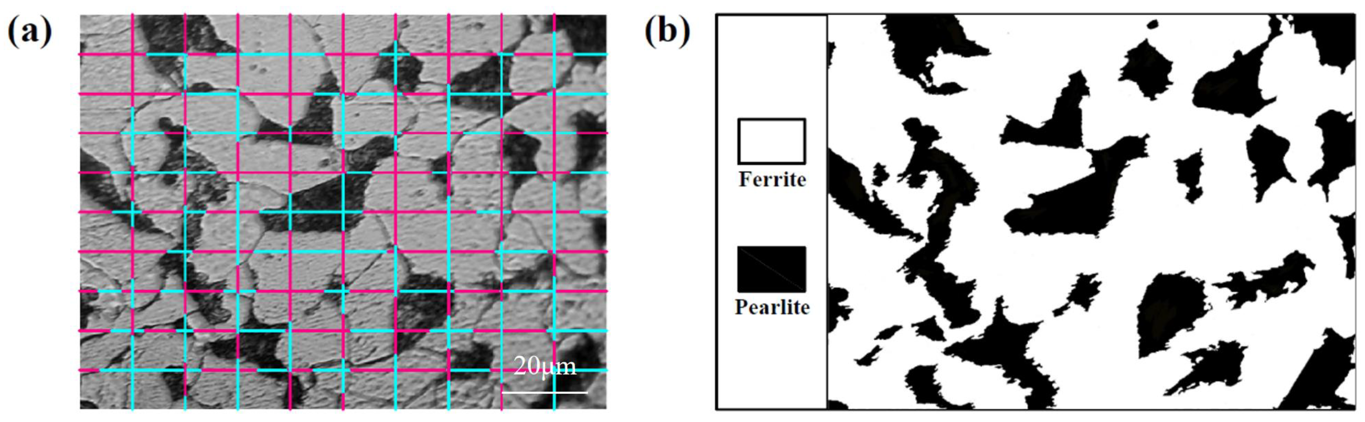
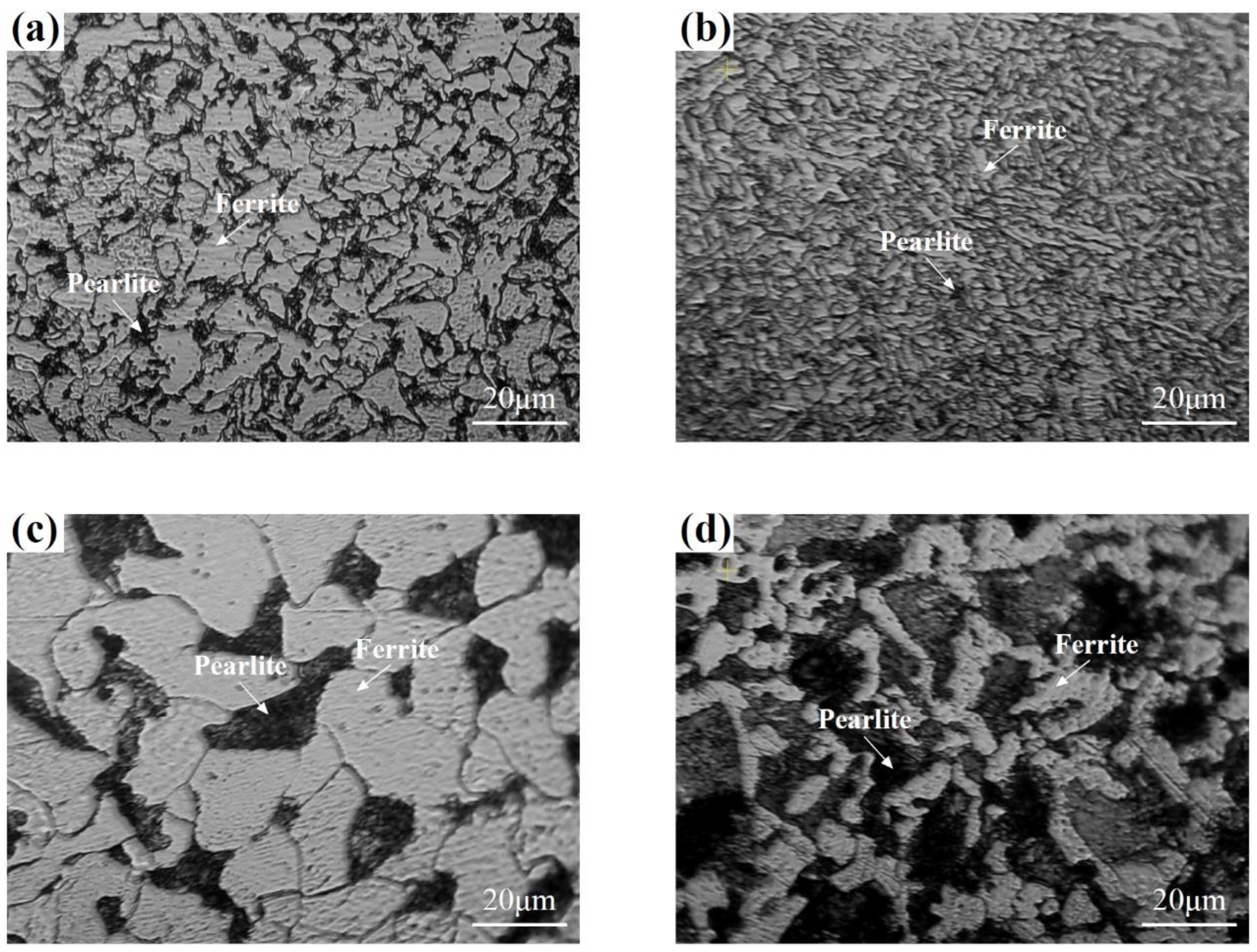
2.1. Measurements on Hardness, Grain Size and Ferrite Volume Fraction

Four BCC steels in Table 1: Q345B, 20 steel, and 45 steel from BaoWu Steel, Shanghai, China, and ER50-G from Golden Bridge Welding Materials, Tianjin are measured in this study. The microstructure of the steels is examined using an optical microscope after polishing and etching with 4% nital solution (4 mL HNO3 and 96 mL alcohol). Vickers hardness is measured by using a Wilson 402 MVD Vickers (Chang’an University, Xi’an, China) hardness tester with different loads (10 g, 25 g, 50 g, 100 g, 200 g, 300 g, 500 g, and 1 kg) with a dwell time of 20 s, and five measurements are performed under each load to get reliable results. According to ASTM E92 [24], the applying load (P) should be greater than 5 kg for H0 measurements. Thus, 10 kg is adopted to obtain H0 using a HV-10 Vickers hardness tester.
Based on the microstructure image, G is measured using the intercept method according to ASTM E112 [25] (Figure 2a). VF is obtained using the method shown in Figure 2b: an optical microstructure picture with two phases is converted to a black–white photo (white area indicates ferrite), and the proportion of the white area is VF [19].

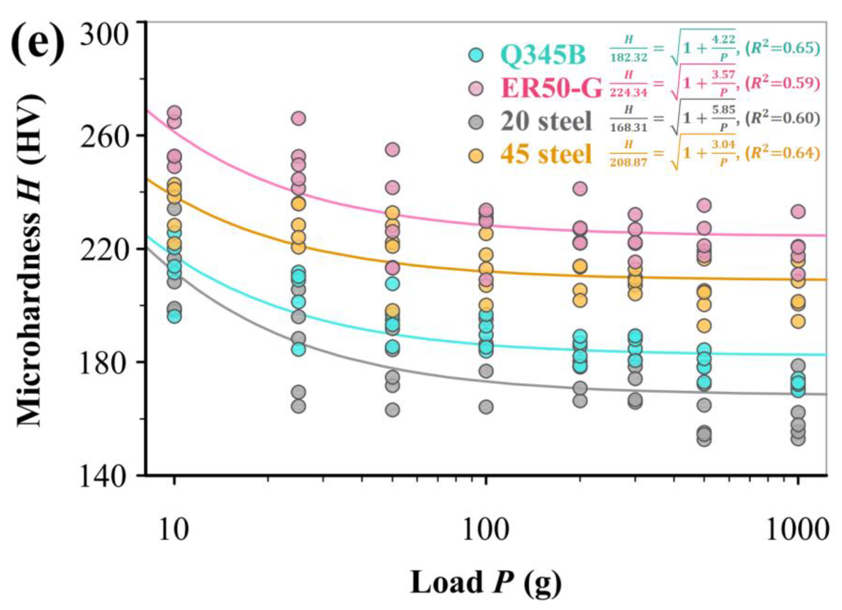
2.2. Experimental Data

Figure 3 shows the observed microstructure and H variation with h value for Q345B, ER50-G, 20 steel and 45 steel. The microstructure, VF, G and H0 of the four steels are listed in Table 2 together with those of other six BCC steels in the literature. It should be mentioned that only the maximum, minimum and mean values under each load are digitized for the hardness data (h, H) on the six BCC steels. The 10 BCC steels consist of up to two metallurgical structures (one of them is ferrite), in which Grade 91 10A and 10B steels consist mainly of martensite and a little ferrite [26,27], the high carbon steel with 0.71% C consists of spheroids cementite and ferrite [28], and the other seven steels consist of pearlite and ferrite.

3. Analytical HH0 Relation by Linking h* to G and VF

To ensure the reliability, the analytical formula describing H/H0 variation with h is proposed based on two different methodologies (theoretical derivation and statistical analysis of experimental data) as shown in Section 3.1 and Section 3.2, respectively. In Section 3.3, the normal distribution analysis is incorporated in the formula to describe the inevitable scatter of measurements under identical conditions.

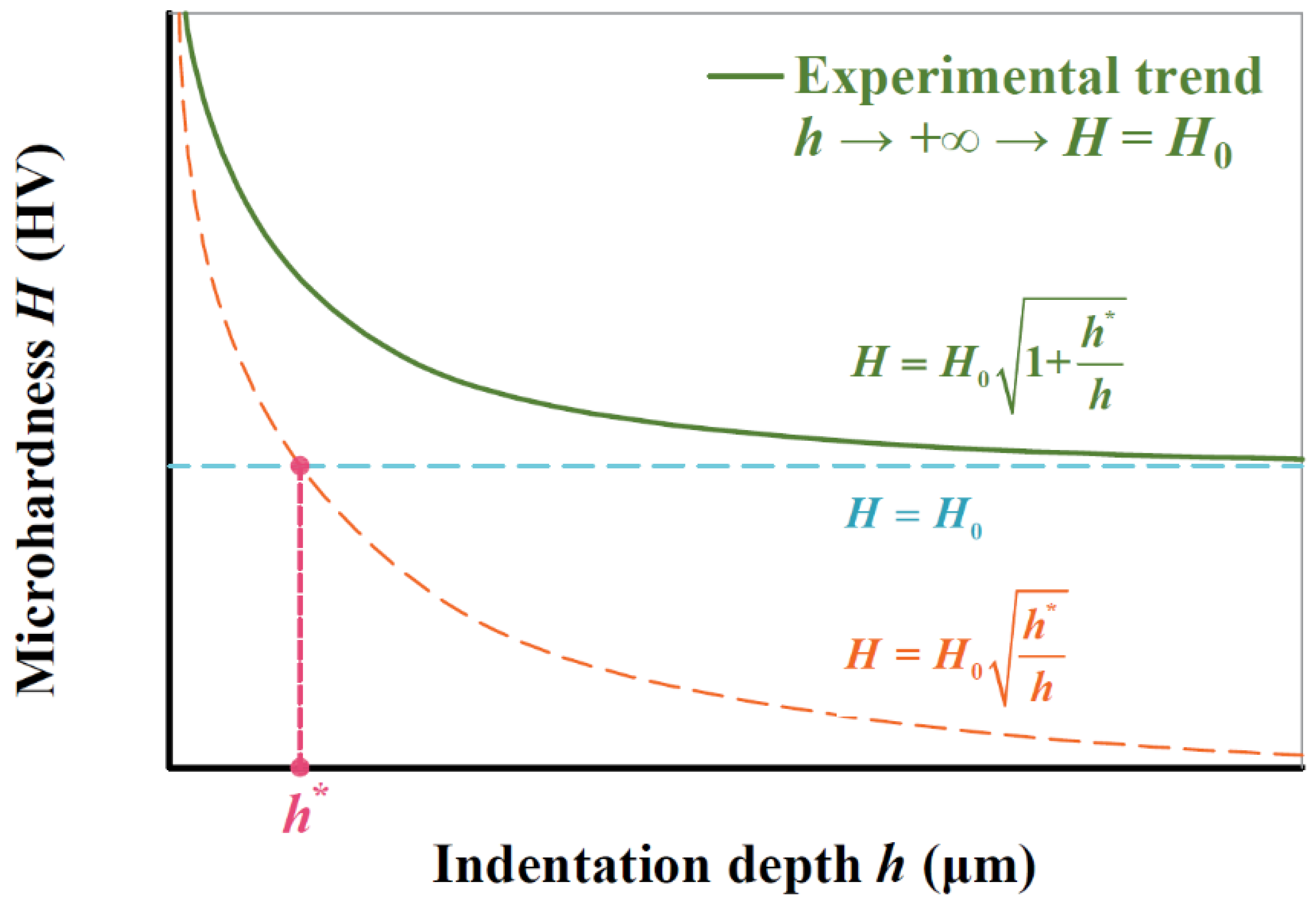
3.1. Theoretical Derivation

The ISE phenomenon during micro- and nano-hardness measurements can be formulated as Equation (1). Recent studies find that h* is related to microstructure, material properties and indenter geometry as follows [10]:
h * = 81 2 1 f 3 α 2 b tan 2 θ ( μ H 0 ) 2
where the scaling factor f = aPDZ/a ≈ 1.9 (aPDZ is the plastic zone size after indenting and a is indentation radius) for steels [32], indenter geometry parameter θ = 22° for Vickers indenter, and α ≈ 0.5, Burgers vector b ≈ 0.248 nm and shear modulus μ ≈ 80 GPa for BCC steels [12].
Yield strength σy of a material includes two parts [33] as follows:
σ y = σ GB + σ 0
where σGB is the contribution of grain boundaries to strength, and σ0 includes precipitation strengthening and solid solution strengthening. In the Hall–Petch relation, σGB is a function of average grain size G [34], as follows:
σ GB = k y G 0.5
where the Hall–Petch coefficient ky can be obtained by data fitting or the following formula [35]:
k y = β μ b
where β is a dimensionless data-fitting parameter. The parameter ky ≈ 20 MPa mm is for steels [36], thus β ≈ 0.5 is calculated based on Equation (5). In numerical terms, the contribution of grain boundaries to hardness (HGB) can be linked to σGB [34,36,37] as follows:
H GB = 3 σ GB = 3 β μ b G 0.5
It is easy to understand that the hardness of a material is pertinent to both metallography organization and grain size. For materials with ferrite, VF has significant influence on the mechanical properties (e.g., hardness, yield strength, and plastic deformation). To consider both G and VF influences, and inspired by the Hall–Patch relation, a concept of relative grain size (Gr) is introduced in this study:
G r = G · e ( V F 1 )
Thus, the following equation can be obtained by replacing G in Equation (6) by Gr:
H GB = 3 β μ b ( G r ) 0.5 = 3 β μ b ( G · e ( V F 1 ) ) 0.5
Similarly, Equation (2) can be rewritten as below by replacing H0 by HGB:
h * = 81 2 1 f 3 α 2 b   tan 2   θ ( μ 3 β μ b ( G · e ( V F 1 ) ) 0.5 ) 2 = 81 α 2   tan 2   θ 18 f 3 β 2 · G · e ( V F 1 )
For BCC steels with α-Fe as matrix, f, θ, and α in Equation (2) and β in Equation (5) are specific, thus h* = 0.107 ≈ 0.1G·e(VF−1). Then, Equation (1) can be rewritten as follows:
H = H 0 1 + 0.1 G · e ( V F 1 ) h

3.2. Analysis of Experimental Data

Based on Taylor’s dislocation model and von Mises rule, tested hardness H resulted from GND and SSD, can be quantified as below [3]:
H = 3 3 α μ b ρ G + ρ S
where ρG is GND density and ρS is SSD density.
In Equation (11), ρG is a function of h [3].
ρ G = 3 2 b h tan 2 θ
When h is infinite or large enough, ρG goes to zero, and H can be regarded as H0. That is, H0 is only governed by SSD, and Equation (11) can be rewritten as follows:
H 0 = 3 3 α μ b ρ S
In Equation (13), ρS can be linked to microstructure [18].
ρ S = 1 c * b L ( 1 e 3 c * ε * )
where L is dislocation mean free path, and the representative strain ε* = 0.2∙tanθ = 0.08 for Vickers indentation tests [18,38], and c* can be obtained by data fitting. For a steel with VF = 100%, LG [19], and the maximum value of L in a steel with VF < 100% is not more than G value [39]. Based on the above discussion, it can be concluded that the L value is closely related to both G and VF for BCC steels. Inspired by this, the following relation is assumed:
L = G · e ( V F 1 )
Combining Equations (11)–(15), the following equation is obtained:
H H 0 = ρ S + ρ G ρ S = 1 + 3 2 b h tan 2 θ 1 e 3 c * ε * c * b G · e ( V F 1 ) = 1 + C · G · e ( V F 1 ) h
where C = 1.5c*tan2θ/(1 − e−0.6c*tanθ).
Comparing Equation (16) with Equation (1), h* = CG·e(VF−1). The difference is that parameter h* in Equation (1) is a data-fitting parameter, and CG·e(VF−1) in Equation (16) has an explicitly physical meaning if C is specific.
As we all know, microhardness measurements on the same material under identical conditions inevitably fluctuate due to material heterogeneity and testing/machining errors. In Equation (16), G and VF are specific for a material, and H and h can be directly obtained for an experiment. Thus, H0 value can be calculated using Equation (16) if C is a constant. It is easy to understand that H0 values should follow normal distribution for a group of measurements on a material. If the C value varies, the corresponding mean and stand deviation values will change for the same group of measurements. From a mathematic point of view, it is reasonable that a minimum of standard deviation (σH0) exists with C variation when C becomes a critical value C0 as illustrated in Figure 4a.
To determine the specific value of C, measurements on low carbon steel (0.19% C), high carbon steel (0.71% C) and Grade 91 10A steel in the literature are analyzed together with measurements on Q345B steel in this study in Figure 4. The corresponding material parameters are listed in Table 2.
Clearly, the standard deviation of H0 (σH0) varies continuously with the C value, and a critical value C0 exists, which corresponds to the minimum of σH0. It can be seen that the C0 value varies from 0.097 to 0.123, and the average of the C0 values approximates 0.109.
Figure 5 shows coefficient of variation (CV = standard-deviation/mean) variation with the C value for the same data in Figure 4, which describes the relative scatter of data. Similarly, CV of H0 varies continuously with the C value, and a critical value C0 exists, which corresponds to the minimum of CV of H0. C0 value varies from 0.094 to 0.112 can be seen, and the average of the C0 values approximates 0.104.
Figure 6 shows the variation in range of (H0)max–(H0)min with the C value for the same data in Figure 4. Again, the minimum of (H0)max–(H0)min occurs when C becomes a critical value C0. The variation in the C0 value from 0.071 to 0.104 can be seen, and the average of the C0 values approximates 0.092.
According to the above analyses, adopting three different mathematical statistical methods for the same measurements (four groups in total), it is found that the critical value C0 fluctuates around 0.1. For simplicity and consistency, it is reasonable to set C0 = 0.1 in this study. Thus, H/H0 variation is successfully described as linked to both G and VF, i.e., h* = 0.1G·e(VF−1). That is, Equation (16) can be rewritten as Equation (10). It should be mentioned that the same equation can be obtained by using different methodologies in Section 3.1 and Section 3.2.

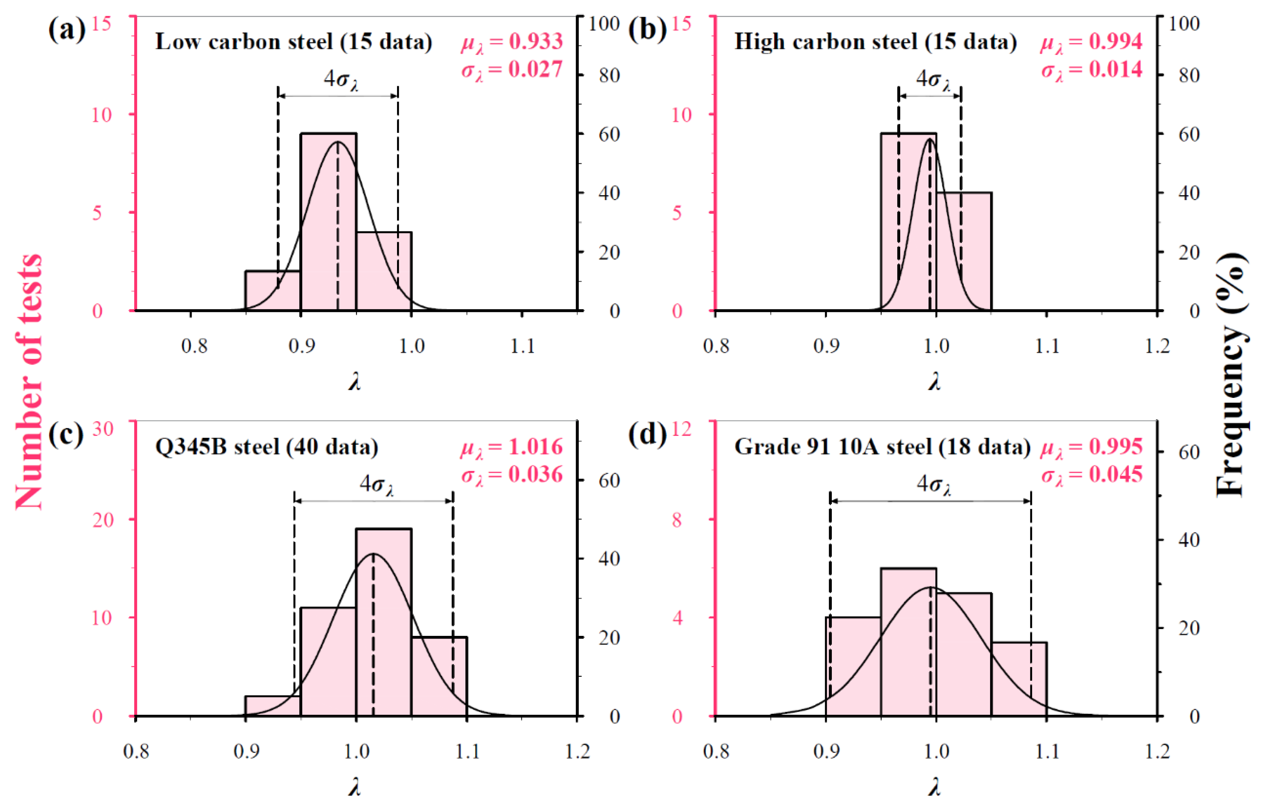
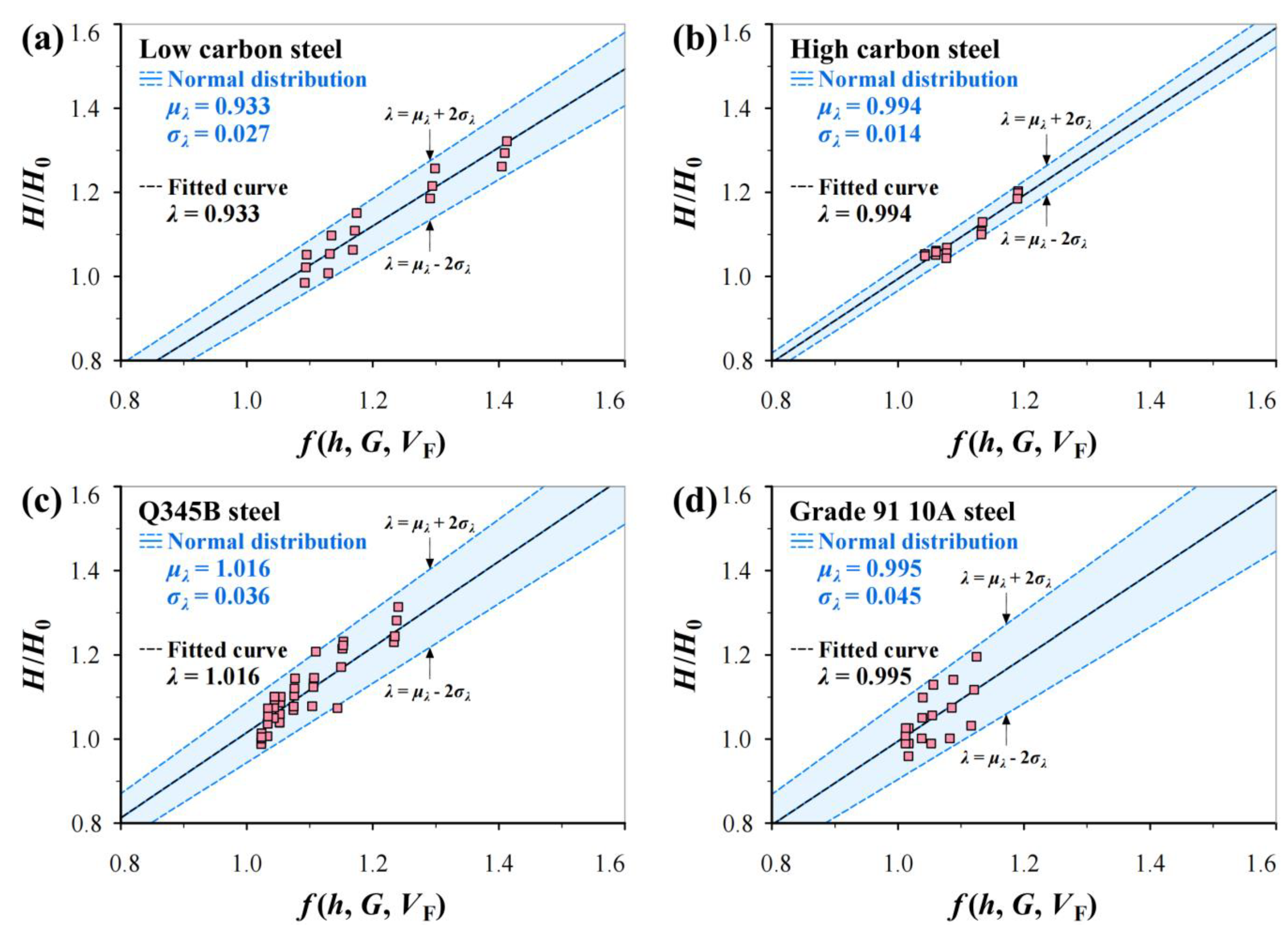
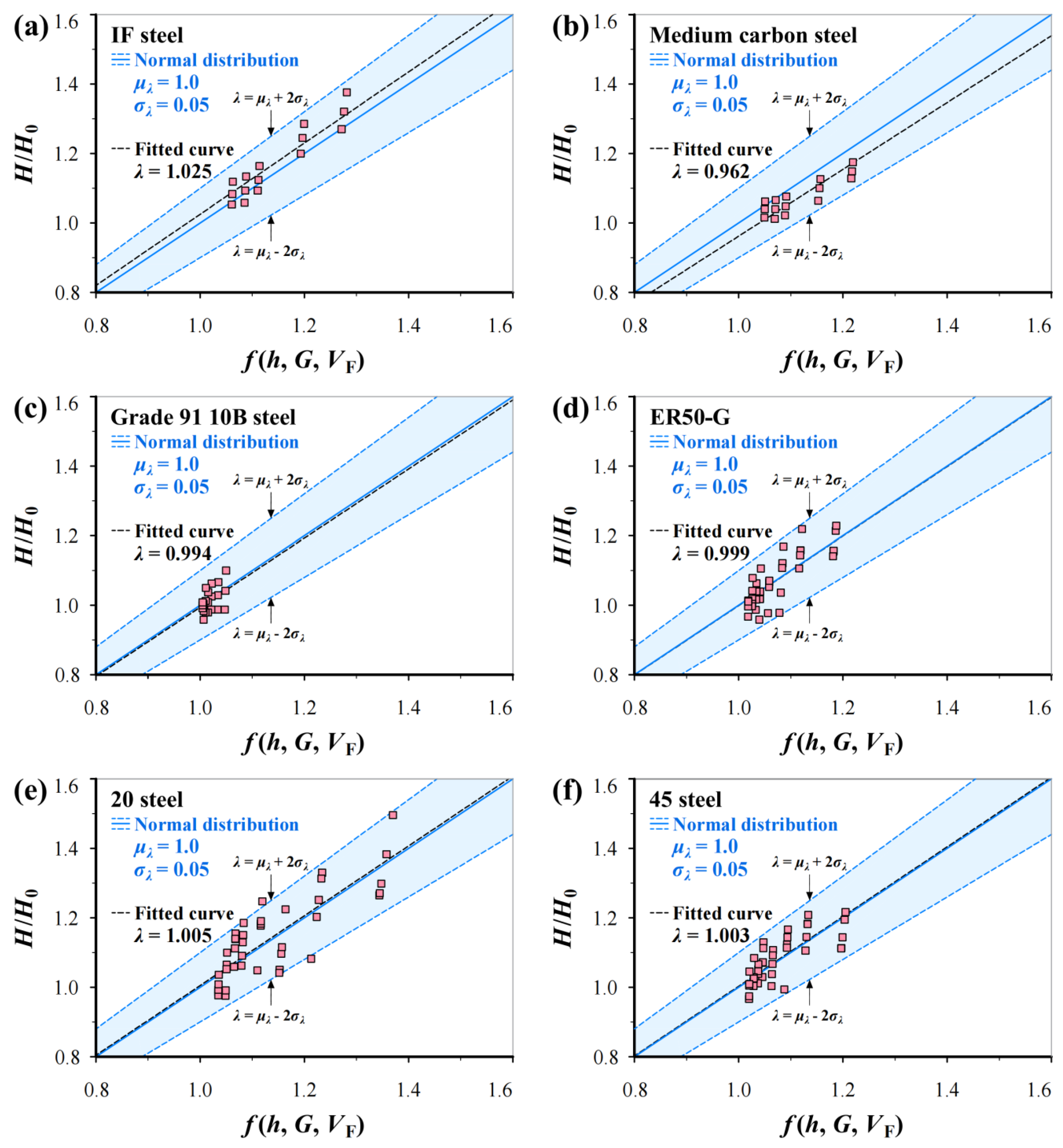
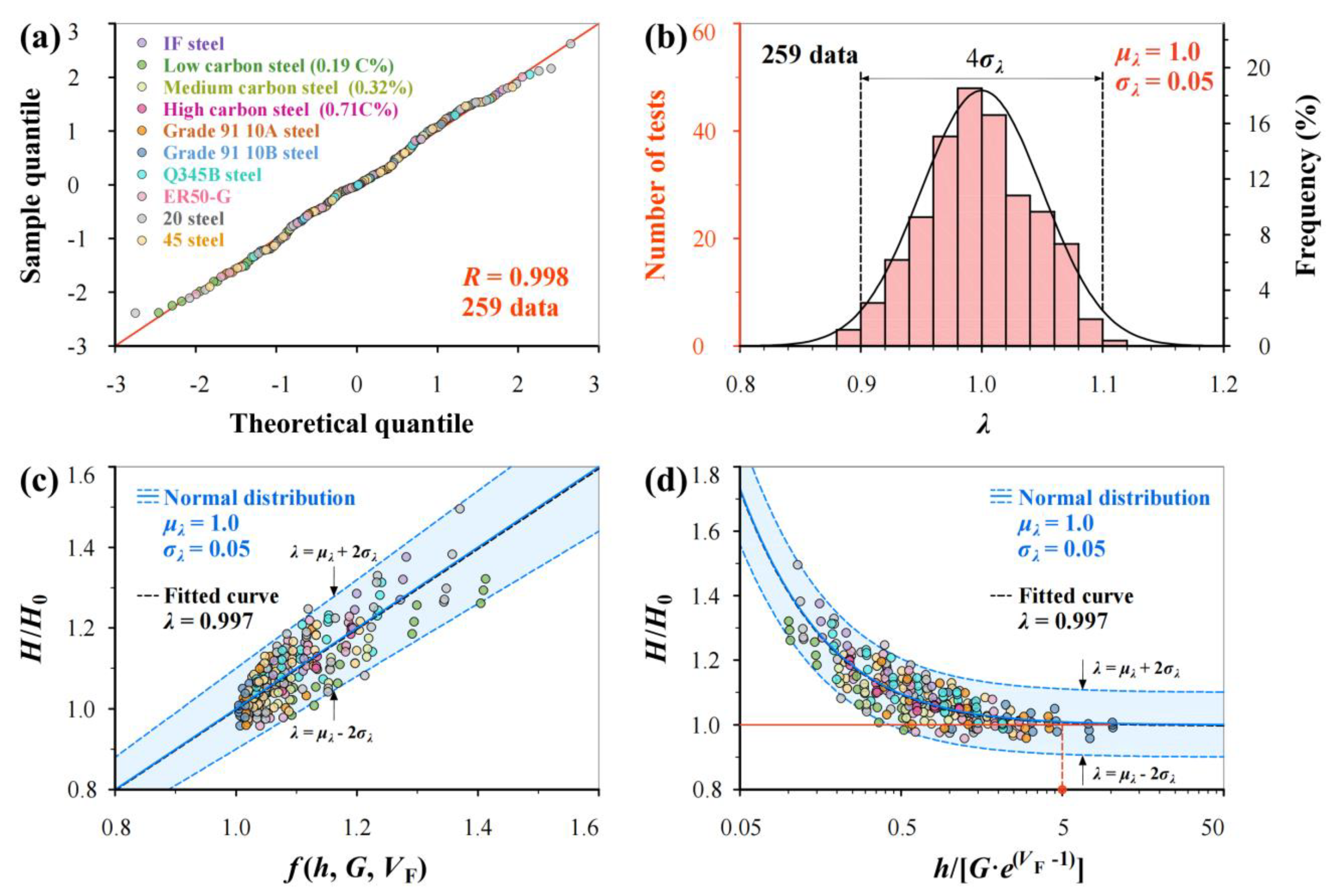
3.3. Normal Distribution Analysis for Inevitable Scatter of H/H0

In theory, the right side of Equation (10) is constant for a material under the same loading conditions, but the tested values of H on the left side inevitably fluctuate because of material heterogeneity and testing/matching errors. For this reason, a non-dimensional parameter λ is incorporated into Equation (10):
H H 0 = λ · 1 + 0.1 G · e ( V F 1 ) h = λ · f ( h ,   G ,   V F )
Obviously, the H/H0 ratio is fully determined by G, VF, and h. For a group of tested H values, corresponding λ values, calculated using Equation (17), can be analyzed using the normal distribution theory to obtain mean μλ and standard deviation σλ. Thus, Equation (17) can be re-reformulated to include both mean, and upper and lower bounds with 96% reliability:
H H 0 = ( μ λ ± 2 σ λ ) · 1 + 0.1 G · e ( V F 1 ) h = ( μ λ ± 2 σ λ ) · f ( h ,   G ,   V F )
To determine the values of μλ and σλ, the four groups of data in Figure 4 are reanalyzed in Figure 7 and Figure 8. It can be seen from Figure 7 that μλ fluctuates from 0.933 to 1.106 and σλ from 0.014 to 0.045. Figure 8 shows the predicted H/H0f(h, G, VF) curves using Equation (18) in linearity using the μλ and σλ values in Figure 7 together with fitted curves for comparison, in which the μλ ± 2σλ values indicate the slopes of three predicted lines. It can be seen that the experimental points are almost covered by the predicted curves, in which the mean curves are nearly identical to fitted curves.
Although μλ fluctuates from 0.933 to 1.106 for the four measurements, it should be 1.0 in theory. Considering the limitation of small sample data, the σλ value should be no less than the maximum of 0.045 in Figure 7. For consistency, the rule of μλ = 1.0 and σλ = 0.05 is set in this study, thus Equation (18) can be rewritten as follows:
H H 0 = ( 1.0 ± 2 × 0.05 ) · 1 + 0.1 G · e ( V F 1 ) h = ( 1.0 ± 2 × 0.05 ) · f ( h ,   G ,   V F )

4. Verification

To validate Equation (19), hardness measurements on six BCC steels in Table 2 are used: IF steel, medium carbon steel (0.32% C) and Grade 91 10B steel in the literature, and ER50-G, 20 steel and 45 steel in this study. Figure 9 shows the predicted H/H0h curves using Equation (19) together with fitted curves and test data for comparison. It can be seen that the predicted curves with mean and upper and lower bounds cover most of the experimental data points.
Figure 10 shows the predicted H/H0f(h, G, VF) curves using Equation (19) in linearity without changing accuracy, in which 1.0 ± 2 × 0.05 indicates the slopes of three predicted lines. It can be seen that the predicted mean curves are very close to the corresponding fitted curves.

5. Discussion

For the micro-indentation hardness test, the ISE phenomenon cannot be ignored. The widely used Nix–Gao model can describe the microhardness variation; however, the empirical parameter h* leads to a limitation of application for testing the material constant. Numerous studies show that tested H is not only related to the h value, but also related to the microstructure and phase content of a material. To investigate the hardness characteristics for BCC steels, which are widely used in industrial applications, h* is explicitly linked to G and VF (h* = 0.1G·e(VF−1)) by two different methods to consider the grain size and phase content. The proposed model can be used to calculate the hardness of a material H0 based on tested data (h, H). Moreover, shallow indentation or low h value has no influence on the calculation accuracy of H0 but can significantly reduce the surface damage of materials or components. Thus, H0 can be easily obtained in microhardness tests with small load.
For BCC steels, larger G and higher VF result in lower dislocation density leading to lower strength and higher plastic deformation capacity. Figure 9 shows that the H/H0–ratio with increasing h more easily approaches the steady state of one for Grade 91 10B steel than other steels. This is because Grade 91 10B has a mainly martensite structure, and VF is lower than other materials, which results in a higher dislocation density. In fact, complex microstructural features such as secondary phases and carbide precipitation significantly affect test results. Thus, the influence of more factors on microhardness variation can be reflected by H. That is why only G and VF are considered part of h* of the Nix–Gao model and good robustness for different BCC steels can be found.
The scatter of hardness measurements under the same loading condition is inevitable due to the micro-heterogeneity of a material, and it increases with decreasing h. Therefore, normal distribution analysis is incorporated into the proposed model. To further validate Equation (19), Figure 11 shows the integrated analysis of measurements on 10 BCC steels. The q-q plot (Figure 11a) of λ values from all 259 data proves that the measurements on different materials still obeys normal distribution, as the correlation coefficient R = 0.998, and the unified normal distribution parameters (μλ = 1.0 and σλ = 0.05) are deemed acceptable by comparing the predicted curves with the histogram from measurements. Clearly, the prediction using Equation (19) agrees well with the experimental data, and the predicted curves with upper and lower bounds (96% reliability) cover most of the experimental points. Equation (19) can be flexibly used in linearity and non-linearity, as shown in Figure 11c,d. In addition, Figure 11d shows that the H/H0 ratio is less than 1.025 when h/[Ge(VF−1)] > 5, in which the tested value H can be regarded as material hardness H0.
In addition, experimental data exhibiting a non-normal distribution can also be analyzed with Weibull distribution or lognormal distribution. For the application of other statistical models or distribution types, the non-dimensional parameters μλ and σλ can be modified by adding a skewness coefficient calculated from data.

6. Conclusions

This study investigates microhardness H variation in BCC steels with indentation depth h during micro-indentation hardness tests by analyzing Vickers microhardness measurements on 10 BCC steels with G from 10.00 μm to 34.41 μm and VF from 5% to 100%. The main conclusions are as follows:
  • Based on the Nix–Gao model, an analytical relation between H/H0 and h is proposed, which can replace the fitting method commonly used. Through the proposed model, the hardness of a material H0 can be calculated based on tested data (h, H) under any loads.
  • The characteristic indentation depth h* indicates the translation from infinite hardness to macrohardness H0 in H-h curve. By two methods, h* is explicitly linked to average grain size G and ferrite volume fraction VF of BCC steels, i.e., h* = 0.1Ge(VF−1).
  • In micro-indentation hardness tests, when the indentation depth h is more than 5Ge(VF−1), the tested value H ≤ 1.025H0 which can be regarded as material hardness H0.
  • Normal distribution theory is incorporated successfully to quantify the inevitable scatter of hardness measurements resulting from the microstructure heterogeneity of a material and machining/testing errors. After considering scatter, this model includes both mean, and upper and lower bounds with 96% reliability, which ensue effective application for material testing and quality control.

Author Contributions

Conceptualization, A.X.; Methodology, M.Y. and C.Z.; Software, M.Y. and Y.W.; Validation, A.X.; Formal analysis, A.X.; Resources, X.S., M.Y. and Y.W.; Data curation, A.X.; Writing—original draft, A.X.; Writing—review & editing, A.X. and C.Z.; Supervision, X.S. and Y.W.; Funding acquisition, C.Z. All authors have read and agreed to the published version of the manuscript.

Funding

This work was supported by the National Natural Science Foundation of China (52375141, 11672048 and 52105398), the Belt and Road Project (DL2022171003L), Shaanxi Province (2022JM-002) and Chang’an University (300102251302).

Institutional Review Board Statement

Not applicable.

Informed Consent Statement

Not applicable.

Data Availability Statement

The raw data supporting the conclusions of this article will be made available by the authors on request.

Conflicts of Interest

The authors declare no conflict of interest.

Nomenclature

HTested hardness or microhardness
H0Material hardness or macrohardness
hIndentation depth
h*Characteristic indentation depth as the translation from infinite hardness to H0
GAverage grain size
VFFerrite volume fraction
bBurgers vector
μShear modulus
θIndenter geometry parameter
fScaling factor
σyYield strength
σGBThe contribution of grain boundaries to strength
σ0The contribution of strengthening other than grain boundaries strengthening.
GrRelative grain size
ρGThe density of geometrically necessary dislocation
ρSThe density of statistically stored dislocation
LDislocation mean free path
λNon-dimensional parameter
μλMean of a group of λ
σλStandard deviation of a group of λ

References

  1. Luo, Q.; Kitchen, M. Microhardness, Indentation Size Effect and Real Hardness of Plastically Deformed Austenitic Hadfield Steel. Materials 2023, 16, 1117. [Google Scholar] [CrossRef] [PubMed]
  2. Broitman, E. Indentation Hardness Measurements at Macro-, Micro-, and Nanoscale: A Critical Overview. Tribol. Lett. 2016, 65, 2–18. [Google Scholar] [CrossRef]
  3. Yang, B.; Vehoff, H. Dependence of nanohardness upon indentation size and grain size—A local examination of the interaction between dislocations and grain boundaries. Acta Mater. 2007, 55, 849–856. [Google Scholar] [CrossRef]
  4. Hu, J.; Sun, W.; Jiang, Z.; Zhang, W.; Lu, J.; Huo, W.; Zhang, Y.; Zhang, P. Indentation size effect on hardness in the body-centered cubic coarse-grained and nanocrystalline tantalum. Mater. Sci. Eng. A 2017, 686, 19–25. [Google Scholar] [CrossRef]
  5. Bond, T.; Badmos, A.; Ahmed, R.A.; Obayemi, J.D.; Salifu, A.; Rahbar, N.; Soboyejo, W.O. Indentation size effects in aluminum and titanium alloys. Mater. Sci. Eng. A 2022, 839, 142542. [Google Scholar] [CrossRef]
  6. Mattucci, M.A.; Cherubin, I.; Changizian, P.; Skippon, T.; Daymond, M.R. Indentation size effect, geometrically necessary dislocations and pile-up effects in hardness testing of irradiated nickel. Acta Mater. 2021, 207, 116702. [Google Scholar] [CrossRef]
  7. Nix, W.D.; Gao, H. Indentation size effects in crystalline materials: A law for strain gradient plasticity. J. Mech. Phys. Solids 1998, 46, 411–425. [Google Scholar] [CrossRef]
  8. Manika, I.; Maniks, J. Size effects in micro- and nanoscale indentation. Acta Mater. 2006, 54, 2049–2056. [Google Scholar] [CrossRef]
  9. Jung, B.; Lee, H.; Park, H. Effect of grain size on the indentation hardness for polycrystalline materials by the modified strain gradient theory. Int. J. Solids Struct. 2013, 50, 2719–2724. [Google Scholar] [CrossRef]
  10. Durst, K.; Backes, B.; Göken, M. Indentation size effect in metallic materials: Correcting for the size of the plastic zone. Scr. Mater. 2005, 52, 1093–1097. [Google Scholar] [CrossRef]
  11. Qu, S.; Huang, Y.; Pharr, G.M.; Hwang, K.C. The indentation size effect in the spherical indentation of iridium: A study via the conventional theory of mechanism-based strain gradient plasticity. Int. J. Plast. 2006, 22, 1265–1286. [Google Scholar] [CrossRef]
  12. Sarangi, S.S.; Lavakumar, A.; Singh, P.K.; Katiyar, P.K.; Ray, R.K. Indentation size effect in steels with different carbon contents and microstructures. Mater. Sci. Technol. 2022, 39, 338–346. [Google Scholar] [CrossRef]
  13. Chicot, D. Hardness length-scale factor to model nano- and micro-indentation size effects. Mater. Sci. Eng. A 2009, 499, 454–461. [Google Scholar] [CrossRef]
  14. Seekala, H.; Bathini, L.; Wasekar, N.P.; Krishnaswamy, H.; Sudharshan Phani, P. A unified approach to quantify the material and geometrical effects in indentation size effect. J. Mater. Res. 2023, 38, 1740–1755. [Google Scholar] [CrossRef]
  15. Qin, J.; Huang, Y.; Hwang, K.C.; Song, J.; Pharr, G.M. The effect of indenter angle on the microindentation hardness. Acta Mater. 2007, 55, 6127–6132. [Google Scholar] [CrossRef]
  16. Shen, F.; Münstermann, S.; Lian, J.A. unified fracture criterion considering stress state dependent transition of failure mechanisms in bcc steels at –196 °C. Int. J. Plast. 2022, 156, 103365. [Google Scholar] [CrossRef]
  17. Liu, Z.; Yang, L.; Zhang, G.; Zhao, L.; Shao, Q.; Huang, D.; Zhu, Y.; Wang, X.; Shen, Z.; Yang, H. Correlation of microstructure and hardness distribution of high-speed train wheels under original and service statuses. Eng. Fail. Anal. 2024, 158, 107994. [Google Scholar] [CrossRef]
  18. Mendas, M.; Benayoun, S.; Miloud, M.H.; Zidane, I. Microhardness model based on geometrically necessary dislocations for heterogeneous material. J. Mater. Res. Technol. 2021, 15, 2792–2801. [Google Scholar] [CrossRef]
  19. Ramazani, A.; Mukherjee, K.; Prahl, U.; Bleck, W. Modelling the effect of microstructural banding on the flow curve behaviour of dual-phase (DP) steels. Comput. Mater. Sci. 2012, 52, 46–54. [Google Scholar] [CrossRef]
  20. Zhang, C.; Hu, X.; Sercombe, T.; Li, Q.; Wu, Z.; Lu, P. Prediction of ceramic fracture with normal distribution pertinent to grain size. Acta Mater. 2018, 145, 41–48. [Google Scholar] [CrossRef]
  21. Zhang, C.; Yang, S. Probabilistic prediction of strength and fracture toughness scatters for ceramics using normal distribution. Materials 2019, 12, 727. [Google Scholar] [CrossRef] [PubMed]
  22. Wang, R.; Gu, H.; Zhu, S.; Li, K.; Wang, J.; Wang, X.; Hideo, M.; Zhang, X.; Tu, S. A data-driven roadmap for creep-fatigue reliability assessment and its implementation in low-pressure turbine disk at elevated temperatures. Reliab. Eng. Syst. Saf. 2022, 225, 108523. [Google Scholar] [CrossRef]
  23. Gu, H.; Wang, R.; Zhu, S.; Wang, X.; Wang, D.; Zhang, G.; Fan, Z.; Zhang, X.; Tu, S. Machine learning assisted probabilistic creep-fatigue damage assessment. Int. J. Fatigue 2022, 156, 106677. [Google Scholar] [CrossRef]
  24. ASTM E92; Standard Test Methods for Vickers Hardness of Metallic Materials. ASTM International: West Conshohocken, PA, USA, 2018.
  25. ASTM E112; Standard Test Methods for Determining Average Grain Size. ASTM International: West Conshohocken, PA, USA, 2012.
  26. Kobayashi, S.; Sawada, K.; Hara, T.; Kushima, H.; Kimura, K. The formation and dissolution of residual δ ferrite in ASME Grade 91 steel plates. Mater. Sci. Eng. A 2014, 592, 241–248. [Google Scholar] [CrossRef]
  27. Ragab, M.; Liu, H.; Ahmed, M.M.Z.; Yang, G.; Lou, Z.; Mehboob, G. Microstructure evolution during friction stir welding of 1Cr11Ni2W2MoV martensitic stainless steel at different tool rotation rates. Mater. Charact. 2021, 182, 11561. [Google Scholar] [CrossRef]
  28. Lavakumar, A.; Sarangi, S.S.; Chilla, V.; Narsimhachary, D.; Ray, R.K. A “new” empirical equation to describe the strain hardening behavior of steels and other metallic materials. Mater. Sci. Eng. A 2021, 802, 140641. [Google Scholar] [CrossRef]
  29. Siefert, J.A.; Shingledecker, J.P.; Parker, J.D. Optimization of Vickers hardness parameters for micro- and macro-indentation of Grade 91 steel. J. Test. Eval. 2013, 41, 778–787. [Google Scholar] [CrossRef]
  30. Yaguchi, M.; Tomobe, M.; Komazaki, S.-I.; Kumada, A. Thickness of small sample for creep property evaluation of 9Cr steel base metal of piping on site. Trans. JSME 2022, 88, 00302. (In Japanese) [Google Scholar] [CrossRef]
  31. Sawada, K.; Kushima, H.; Tabuchi, M.; Kimura, K. Microstructural degradation of Gr.91 steel during creep under low stress. Mater. Sci. Eng. A 2011, 528, 5511–5518. [Google Scholar] [CrossRef]
  32. Cui, L.; Yu, C.; Jiang, S.; Sun, X.; Peng, R.; Lundgren, J.; Moverare, J. A new approach for determining GND and SSD densities based on indentation size effect: An application to additive-manufactured Hastelloy X. J. Mater. Sci. Technol. 2022, 96, 295–307. [Google Scholar] [CrossRef]
  33. Iza-Mendia, A.; Gutiérrez, I. Generalization of the existing relations between microstructure and yield stress from ferrite-pearlite to high strength steels. Mater. Sci. Eng. A 2013, 561, 40–51. [Google Scholar] [CrossRef]
  34. Hall, E.O. The deformation and ageing of mild steel: III Discussion of results. Proc. Phys. Soc. 1951, 64, 747. [Google Scholar] [CrossRef]
  35. Jiang, L.; Fu, H.; Zhang, H.; Xie, J. Physical mechanism interpretation of polycrystalline metals’ yield strength via a data-driven method: A novel Hall-Petch relationship. Acta Mater. 2022, 231, 117868. [Google Scholar] [CrossRef]
  36. Seok, M.; Choi, I.; Moon, J.; Kim, S.; Ramamurty, U.; Jang, J. Estimation of the Hall-Petch strengthening coefficient of steels through nanoindentation. Scr. Mater. 2014, 87, 49–52. [Google Scholar] [CrossRef]
  37. Tabor, D. The hardness and strength of metals. J. Inst. Met. 1951, 79, 1–18. [Google Scholar]
  38. Hernot, X.; Moussa, C.; Bartier, O. Study of the concept of representative strain and constraint factor introduced by Vickers indentation. Mech. Mater. 2014, 68, 1–14. [Google Scholar] [CrossRef]
  39. Gutierrez, I. AME modelling the mechanical behaviour of steels with mixed microstructures. J. Metall. Mater. Eng. 2005, 11, 201–214. [Google Scholar]
Figure 1. Nix–Gao model showing H variation with h.
Materials 17 02371 g001
Figure 2. Illustrations of measuring (a) average grain size G and (b) ferrite volume fraction VF for 20 steel.
Materials 17 02371 g002
Figure 3. Microstructure of (a) Q345B, (b) ER50-G, (c) 20 steel and (d) 45 steel, and (e) Vickers microhardness variation with applying load.
Materials 17 02371 g003aMaterials 17 02371 g003b
Figure 4. (a) Illustration of H0 variation with C value based on Equation (16) for (b) low carbon steel (0.19% C), (c) high carbon steel (0.71% C), (d) Grade 91 10A steel, and (e) Q345B steel.
Materials 17 02371 g004
Figure 5. (a) Illustrating the CV variation with C value based on Equation (16) for (b) low carbon steel (0.19% C), (c) high carbon steel (0.71% C), (d) Grade 91 10A steel, and (e) Q345B steel.
Materials 17 02371 g005
Figure 6. (a) Illustrating the variation in range of (H0)max–(H0)min with C value based on Equation (16) for (b) low carbon steel (0.19% C), (c) high carbon steel (0.71% C), (d) Grade 91 10A steel, and (e) Q345B steel.
Materials 17 02371 g006
Figure 7. Histograms and frequencies of λ distributions from measurements on (a) low carbon steel (0.19% C), (b) high carbon steel (0.71% C), (c) Q345B steel, and (d) Grade 91 10A steel.
Materials 17 02371 g007
Figure 8. Predicted H/H0f(h, G, VF) relations using Equation (18) in linearity using μλ and σλ values in Figure 7 together with fitted curves: (a) low carbon steel (0.19% C), (b) high carbon steel (0.71% C), (c) Q345B steel, and (d) Grade 91 10A steel.
Materials 17 02371 g008
Figure 9. Predicted H/H0h relations using Equation (19) together with fitted curves and experimental data: (a) IF steel, (b) medium carbon steel (0.32% C), (c) Grade 91 10B steel, (d) ER50-G, (e) 20 steel, and (f) 45 steel. The red line indicates a trend line.
Materials 17 02371 g009
Figure 10. Predicted H/H0f(h, G, VF) relations using Equation (19) in linearity together with fitted curves and experimental data: (a) IF steel, (b) medium carbon steel (0.32% C), (c) Grade 91 10B steel, (d) ER50-G, (e) 20 steel, and (f) 45 steel.
Materials 17 02371 g010
Figure 11. Integrated analysis of hardness measurements on 10 BCC steels. (a) q-q plot, (b) the histogram of λ values from total of 259 data and normal distribution prediction with μλ = 1.0 and σλ = 0.05, (c) predicted H/H0f(h, G, VF) relations in linearity and (d) predicted H/H0h/[G·e(VF−1)] curves using Equation (19) together with fitted curve and experimental data.
Materials 17 02371 g011
Table 1. Chemical compositions of materials tested in this study (in wt. %).
MaterialsCSiMnPSCuCrNiFe
Q345B0.140.51.70.0350.0350.300.30.05Balance *
ER50-G0.070.91.50.0120.0110.50.020.02Balance
20 steel0.20.220.530.0350.0350.070.040.01Balance
45 steel0.450.170.50.0350.0350.250.250.25Balance
* Balance: The proportion of elements other than those already listed.
Table 2. Material parameters of BCC steels used in this study [12,26,28,29,30,31].
MaterialsPhaseVFG (μm)H0 (HV)
Q345BF * + P *84%8.17171.9
ER50-GF + P94%5.19218.2
20 steelF + P76%14.14156.6
45 steelF + P43%10.01199.5
IF steel [12]F100% [28]24.29 [12]94.5 [12]
Low carbon steel (0.19% C) [12]F + P72% [28]34.41 [12]206.7 [12]
Medium carbon steel (0.32% C) [12]F + P58% [28]19.23 [12]237.0 [12]
High carbon steel (0.71% C) [12]F + SC *56%16.43 [12]244.1 [12]
Grade 91 10A steel [29]F + M *5% [26]30.00 [30]164.7 [29]
Grade 91 10B steel [29]F + M5% [26] 10.00 [31]240.0 [29]
* Ferrite (F), pearlite (P), spheroidal cementite (SC), and martensite (M).
Disclaimer/Publisher’s Note: The statements, opinions and data contained in all publications are solely those of the individual author(s) and contributor(s) and not of MDPI and/or the editor(s). MDPI and/or the editor(s) disclaim responsibility for any injury to people or property resulting from any ideas, methods, instructions or products referred to in the content.

