Abstract
With the rapid development of renewable energy and the increasing maturity of energy storage technology, microgrids are quickly becoming popular worldwide. The stochastic scheduling problem of microgrids can increase operational costs and resource wastage. In order to reduce operational costs and optimize resource utilization efficiency, the real-time scheduling of microgrids becomes particularly important. After collecting extensive data, reinforcement learning (RL) can provide good strategies. However, it cannot make quick and rational decisions in different environments. As a method with generalization ability, meta-learning can compensate for this deficiency. Therefore, this paper introduces a microgrid scheduling strategy based on RL and meta-learning. This method can quickly adapt to different environments with a small amount of training data, enabling rapid energy scheduling policy generation in the early stages of microgrid operation. This paper first establishes a microgrid model, including components such as energy storage, load, and distributed generation (DG). Then, we use a meta-reinforcement learning framework to train the initial scheduling strategy, considering the various operational constraints of the microgrid. The experimental results show that the MAML-based RL strategy has advantages in improving energy utilization and reducing operational costs in the early stages of microgrid operation. This research provides a new intelligent solution for microgrids’ efficient, stable, and economical operation in their initial stages.
1. Introduction
With the rise in worldwide energy consumption and the growing prominence of environmental concerns, governments and research institutions worldwide are paying more attention to developing renewable energy technologies. This trend aims to modify the energy structure and foster the sustainable advancement of society. Renewable energy sources, such as solar, wind, geothermal, and biomass, act as alternatives to conventional fossil fuels and can significantly reduce carbon emissions. Distributed generation technologies based on these energy sources are receiving high academic attention [1,2,3,4].
In simple terms, a microgrid is a small-scale power system that can operate independently of the traditional grid or be interconnected with it. Microgrids typically include various renewable energy sources, such as solar and wind power, energy storage devices, conventional generators, and loads [5,6,7]. As an innovative way of supplying energy, microgrids can integrate multiple energy sources to achieve a more efficient, stable, and sustainable power supply. The core value of microgrids lies in their ability to integrate and optimally configure various energy sources [8]. However, the high complexity and uncertainty of microgrids make their scheduling and management a significant challenge. Compared to traditional microgrids, microgrids have greater flexibility and response speeds, allowing them to react quickly to emergencies and load changes. However, this flexibility also brings more uncertainty, especially considering the weather dependency of renewable energy sources [9,10].
Various methods for controlling microgrid scheduling have emerged with the prevalence of microgrids. One of the earliest methods is rule-based scheduling, which defines how to schedule different resources under specific circumstances. In the work of Dimeas and Hatziargyriou [11], they proposed a microgrid control method based on multi-agent systems and algorithms for the fair allocation problem, achieving optimal energy exchange between production units, local loads, and the main grid in the microgrid. Logenthiran et al. [12] proposed the exploration of multi-agent coordination of Distributed Energy Resources (DERs) in microgrids, emphasizing the importance of defining clear operating rules based on the real-time status of the microgrid, such as load demand, renewable energy output, and the state of energy storage devices. In their research, Li et al. [13] focused on the application field of smart home control, using rule-based methods for scheduling and managing devices. Lasseter and Paigi [14] delved into the characteristics of microgrids as a conceptual solution. They discussed how microgrids can operate autonomously, interact with the traditional grid, or operate independently during a power outage through predefined rules and strategies.
The core advantage of Model Predictive Control (MPC) lies in its ability to self-correct uncertain predictions of the model and adaptively adjust the control sequence [15]. It continuously optimizes its predictive model within a rolling time window. Many successful examples demonstrate the effectiveness of MPC in the energy management of microgrids. Molderink et al. [16] studied the management and control of smart grid technology for households, adopting an MPC strategy to implement a three-step control method, including local forecasting, global planning, and real-time local control to schedule different household devices for more efficient energy use. Parisio et al. [17] proposed a method based on MPC to optimize the operation of microgrids, conducting an in-depth exploration of different energy assets within the microgrid, aiming to maximize economic benefits and ensure stable operation. Garcia-Torres et al. [18] published an article on the MPC of microgrid functionalities, discussing the applications and advantages of MPC in microgrids, summarizing the prospects of its application, and proposing future issues and challenges that need to be addressed. While the above methods have achieved certain success in the control of microgrids, they all have their drawbacks. Rule-based scheduling methods need more flexibility and adaptability, and MPC methods rely on accurate mathematical models of the system.
Reinforcement learning (RL) [19] is an adaptive learning method that operates through a “trial-and-error” approach. RL algorithms continuously interact with the environment, perceiving the state of the environment and implementing corresponding control strategies to alter that state [20]. Subsequently, based on the rewards received, the agent updates model parameters to maximize cumulative reward returns. Through this cycle of perception, action, evaluation, and learning, the agent progressively refines its strategy to adapt to changes in the environment and identifies the optimal strategy. RL has been widely applied in various fields, including autonomous driving [21,22], robotic control [23], and gaming [24]. Using RL for microgrid scheduling has the advantage of improving the efficiency of the microgrid and enhancing its adaptability to environmental and market changes. Many papers have demonstrated the feasibility of using RL for energy management in microgrids. Bui et al. [25] proposed a new approach that combines centralized and decentralized energy management systems and applied Q-learning to the operational strategy of Community-Based Energy Storage Systems in microgrid systems. This approach can enhance the efficiency and dependability of microgrid systems while reducing learning time and improving operational outcomes. The research in the paper has important theoretical and practical significance for intelligent energy management in microgrid systems. Alabdullah and Abido [26] proposed a method based on deep RL for solving the energy management problem of microgrids. By implementing an efficient deep Q-network algorithm, this method can schedule diverse energy resources within the microgrid in real time and implement cost-effective measures under uncertain conditions. The research results show that the proposed method is close to optimal operating cost results and has a short computation time, demonstrating the potential for real-time implementation. Mu et al. [27] proposed using a multi-objective interval optimization scheduling model and an improved DRL algorithm called TCSAC to optimize microgrids’ economic cost, network loss, and branch stability index. The effectiveness of the proposed method was verified through simulation results, rendering it a significant asset for scholars and practitioners in the domain of smart grid technology.
RL offers significant advantages in multi-objective optimization and real-time decision-making in microgrid scheduling. By using RL, microgrid energy management systems can achieve adaptive regulation, enhance system flexibility and robustness, optimize energy usage efficiency, reduce operational costs, and improve adaptability to external changes such as weather variations and market price fluctuations. However, there are notable drawbacks, such as the requirement for extensive training data and a lack of capability to rapidly adapt to new environments.
With the development of artificial intelligence and machine learning technology, meta-learning has become an essential branch of machine learning, attracting much attention due to its many advantages, such as fast adaptation to new tasks and low data requirements [28,29,30]. The goal of meta-learning is to enable models to accumulate experience during the learning process and utilize this experience to quickly adapt to new tasks or environments, thereby reducing dependence on extensive labeled data and enhancing learning efficiency. The essence of meta-learning lies in enabling models to learn general knowledge across a series of related tasks, allowing them to rapidly adjust parameters with minimal data during iterations when encountering new tasks. Meta-learning has been widely applied across multiple fields. In natural language processing, meta-learning can help models quickly adapt to new languages, dialects, or specific domain texts, improving the model’s performance in few-shot learning and cross-lingual transfer learning [31]. In image recognition, meta-learning is used to train efficient classifiers with only a few labeled samples [32]. Meta-learning is particularly important for medical image analysis and biometric recognition, where obtaining a large amount of labeled data is often difficult or expensive. In fields such as autonomous driving and weather forecasting, meta-learning can be used to quickly adjust model parameters under different environments or conditions, ensuring the stability and accuracy of the model [33].
The generalization ability of meta-learning, which allows for quick learning from past experiences and adaptation to new tasks, can effectively compensate for the deficiencies of RL in microgrid scheduling. Consequently, this paper proposes a method for real-time microgrid scheduling that combines meta-learning with RL. The contributions of this article to the research field are shown below.
1. This paper proposes a novel algorithm based on Model-Agnostic Meta-Learning (MAML) and Soft Actor–Critic (SAC), Model-Agnostic Meta-Learning for Soft Actor–Critic (MAML-SAC), which is able to quickly adapt to new microgrid environments with a small amount of training data. Compared to the Soft Actor–Critic algorithm, the algorithm proposed in this paper makes better decisions in the early stage of microgrid operation with scarce data.
2. This paper provides new ideas for the real-time scheduling of microgrids. The algorithm of meta-reinforcement learning is used for decision-making at the beginning of microgrid operation when data is scarce. As the amount of data increases, RL is applied at appropriate times for training and decision-making.
3. In the proposed meta-reinforcement learning framework, we introduce a dynamic learning rate adjustment mechanism and residual connection technology to promote the effective flow of information and the efficient propagation of gradients. Integrating these techniques enables the algorithm to adapt quickly to new environments, improving learning efficiency and generalization ability.
4. RL methods typically require a large amount of training data from the current environment for prolonged training. In contrast, the meta-reinforcement learning method proposed in this paper achieves microgrid optimization scheduling in a short time by pre-training and fine-tuning.
The rest of the paper is organized as follows: Section 2 introduces the components of a microgrid and describes the problem in mathematical terms. Section 3 presents our proposed MAML-SAC model. Section 4 presents the experimental setup and experimental results. Finally, we give conclusions and summarize in Section 5.
2. Microgrid Modeling and Problem Formulation
A typical microgrid consists of an Energy Storage System (ESS), Distributed Generators (DGs), and loads. The microgrid can exchange power with the main grid when connected. The time slot duration for power scheduling is commonly set at t = 1 h, with a total of T time slots in each scheduling period, typically selected as 24 time slots, corresponding to 1 day [34].
2.1. Operation Cost Models
(1) Generator operating cost: The operating cost of a generator is mainly fuel expenses, primarily determined by the generator’s power output. Generally, the generation cost can be represented by a quadratic function of power, which yields:
where a, b, and c are parameters for each generator. A generator’s startup and shutdown costs can be set as constant expenses. However, in microgrids, the generators are generally small, and the startup and shutdown costs can be negligible compared to the consumption during the generation process.
(2) Cost of power exchange with the main grid: The selling price of power from the microgrid to the public grid is lower than the purchase price, which is determined by the discount factor . When using electricity data, we consider the real-time electricity market. Assuming the real-time electricity price is , the cost of power exchange is:
(3) Load penalty: There is a high penalty for load shedding. It should be avoided. The amount of the penalty is proportional to the amount of load that is not met:
where is the penalty factor.
2.2. Operation Constraints
(1) Generation of a DG: the power constraint of the generator is:
(2) Ramp Constraints of a DG: The output power of the generator cannot change arbitrarily and is subject to Ramp Constraints:
(3) Power exchange limitation: The exchangeable power between the microgrid and the public grid is limited. The power exchange constraint is:
(4) Constraints on energy storage: We set the upper and lower boundaries of the ESS to prevent overcharging or discharging:
The limitations on charging and discharging can be expressed as:
The description of the ESS should be as follows:
where and are the charging and discharging efficiency coefficients and they are in the range (0, 1).
(5) Assuming there are n generators and m ESSs, the following constraint applies to any t to achieve power balance:
The superscript i denotes the i-th unit within specific group.
2.3. The Optimization Problem
The total operating cost at each time step t can be calculated as:
The optimization problem in the microgrid scheduling aims to minimize the cumulative cost over a scheduling horizon of T time steps. This can be formulated as:
As is common in the literature, transmission power losses and the calendar degradation of batteries are neglected in this model.
3. The Framework of the Proposed Method
3.1. Markov Decision Process (MDP)
A Markov process is a stochastic process in which the probability distribution of future states is solely contingent upon the present state and not on the sequence of preceding states. This property is called “memorylessness” or “Markov property”. The problem described in the previous chapter can be formulated as a Markov process and modeled as a quintuple . S represents the set of system states. A represents the set of actions. P represents the state transition probabilities, where denotes the probability of transitioning from state s to state s′ under action a. R represents the reward function, where R(s, a) denotes the reward received after taking action an in-state s. is the discount factor, ranging from 0 to 1. A larger value of places more emphasis on long-term accumulated rewards. This Markov process formulation is frequently employed in RL to model decision-making scenarios in which an agent engages with an environment to maximize cumulative reward.
3.2. MDP Modeling of Microgrid Environments
In the Markov process, the RL agent controls energy scheduling, and the state information serves as a crucial foundation for the agent. We define the state space as follows: , where t is the timestamp, p is the electricity price of the main grid, soc is the remaining energy of the ESS, is the current load, and is the power generation of the generator. The action space for the agent to control energy scheduling is , where is the charging/discharging power of the ESS, and is the status of the generator. The agent cannot control the exchange power between the microgrid and the main grid. After taking action, the main grid balances the load by inputting/outputting electrical energy, and there is a maximum power limit for input and output.
In time t, given the state and action , the probability of the system transitioning to the next state is denoted by the state transition probability:
In RL, the reward r is provided by the environment and guides the direction of policy updates. In the microgrid optimization scheduling problem discussed in this paper, the reward function should direct the agent to take actions that reduce operating costs.
In the microgrid optimization problem context, the cost C(t), i.e., C(t) in (14), represents the expenses associated with purchasing electricity from the main grid and the operation of generators. The term represents the imbalance at time t, which could be due to a shortage or surplus of electricity. The parameters and balance the trade-off between minimizing costs and penalizing power imbalances. The RL algorithm aims to find an optimal scheduling policy that maximizes the total expected discounted reward over the defined MDP. This involves making decisions that minimize costs and balance supply and demand in the microgrid.
3.3. MAML-SAC
Based on RL, the Soft Actor–Critic (SAC) algorithm has advantages in microgrid applications, such as real-time decision-making and control, multi-objective optimization, strong robustness, and efficient energy management. However, RL methods still face challenges, such as low sample efficiency and the need for accurate environmental models.
A combined approach of Model-Agnostic Meta-Learning (MAML) and SAC, called MAML-SAC, has been proposed to tackle these challenges. MAML is a meta-learning method that enables fast adaptation to new tasks with a small amount of data, which can help improve sample efficiency. By integrating MAML with SAC, the MAML-SAC method can leverage the strengths of both approaches, enabling more efficient and effective learning and decision-making in microgrid energy management.
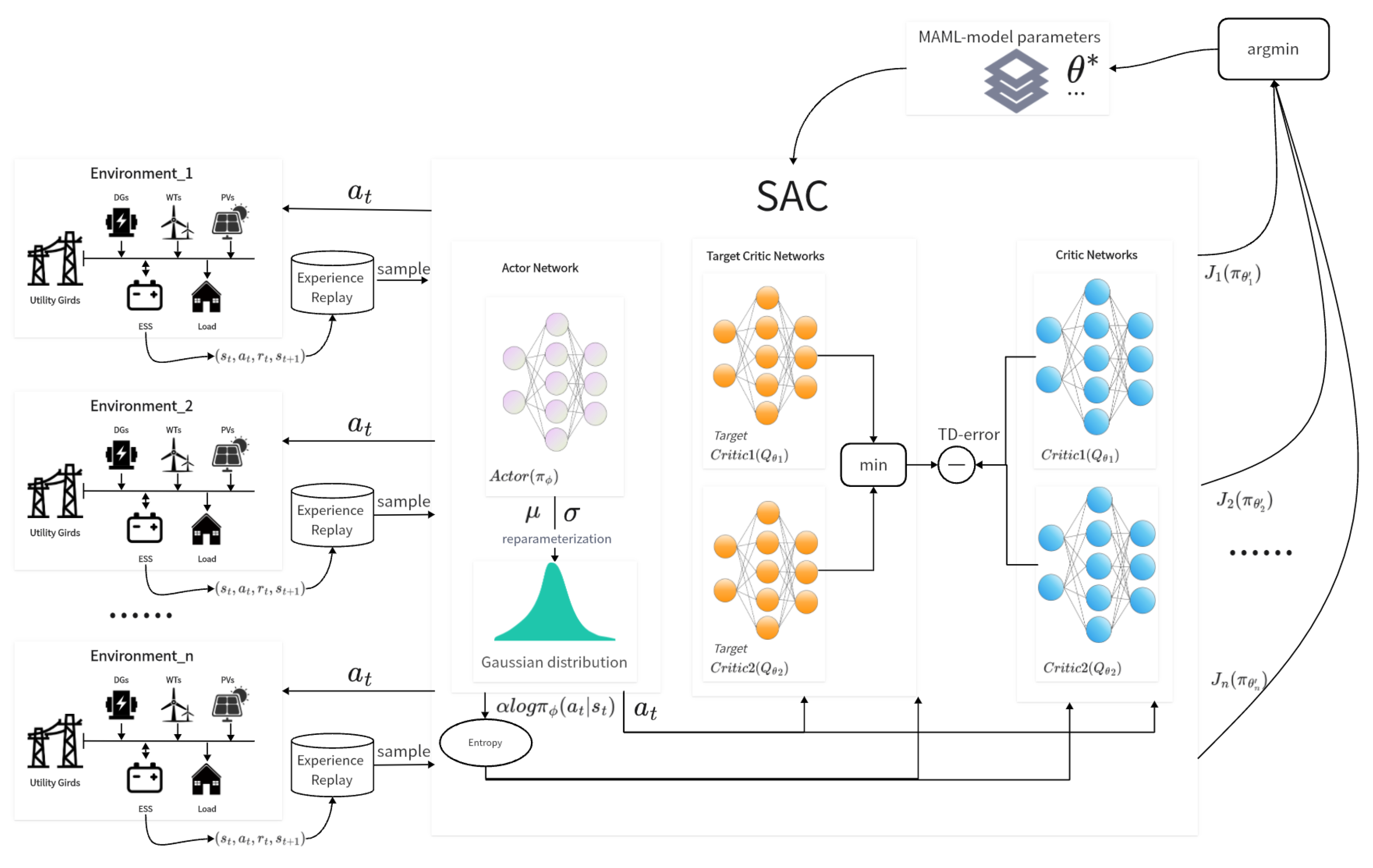
Figure 1 shows the training process of the MAML-SAC model. The first step in the MAML-SAC approach for microgrid control is task sampling. This step randomly sampled a series of microgrid tasks from the task distribution. These tasks can vary based on different factors such as time, internal conditions of the microgrid, and other variables that represent different operating scenarios. This sampling process is crucial for ensuring that the model is subjected to a wide array of scenarios, which helps in learning a generalizable set of initial parameters that can quickly adapt to new tasks.
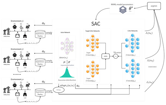
Figure 1.
The training process of the MAML-SAC model.
The next step is model initialization. This step selects an RL model suitable for the microgrid optimization problem. For the MAML-SAC approach, the SAC architecture is chosen due to its ability to handle continuous action spaces and its balance between exploration and exploitation. The model parameters, including those of the policy network and the Q-network, are then initialized. These initial parameters serve as the subsequent steps’ starting point for the adaptation process. The goal is to learn a set of initial parameters that can be quickly fine-tuned to perform well on new tasks with minimal additional training.
The training process in the MAML-SAC approach for microgrid control is divided into two main loops: the inner loop (fast adaptation) and the outer loop (meta-learning update). The inner loop of the MAML-SAC approach involves the following steps for each sampled task: (1) exploration and data collection: The current policy is executed to interact with the microgrid environment, collecting data on states, actions, rewards, and the next states. This step is crucial for gathering the experience necessary to adapt the policy to the specific task. (2) Gradient update: Based on the collected data, the gradient of the policy is computed and the model parameters are updated. The number of updates is usually kept small to enable quick adaptation to the task. In the case of SAC, this involves updating both the policy network and the Q-network. (3) Policy evaluation: The adapted policy is tested on different instances of the same task to evaluate the model’s adaptability. This step assesses how well the model has adapted to the task with the limited updates performed in the previous step. These steps are repeated for each task in the batch, allowing the model to adapt to various microgrid operating scenarios. The goal is to learn initial parameters that can be quickly fine-tuned for effective performance on new tasks.
After completing the inner loop, the model’s performance across multiple tasks adjusts the meta-learning parameters. This typically involves the following steps: (1) loss function aggregation: The average loss across multiple tasks is aggregated, which reflects how well the model adapts to new tasks. This aggregated loss is used to guide the meta-update. (2) Meta-update: Gradient descent is used to update the meta-parameters. This step aims to improve the model’s ability to quickly adapt to new tasks. The meta-parameters are updated in a direction that reduces the aggregated loss, which indicates better adaptability. The process of repeating the inner and outer loop continues until the agent’s performance reaches a satisfactory level. Through this iterative process, the model learns a set of initial parameters that can be effectively fine-tuned to perform well on various microgrid operating scenarios, enhancing the flexibility and efficiency of the microgrid control system.
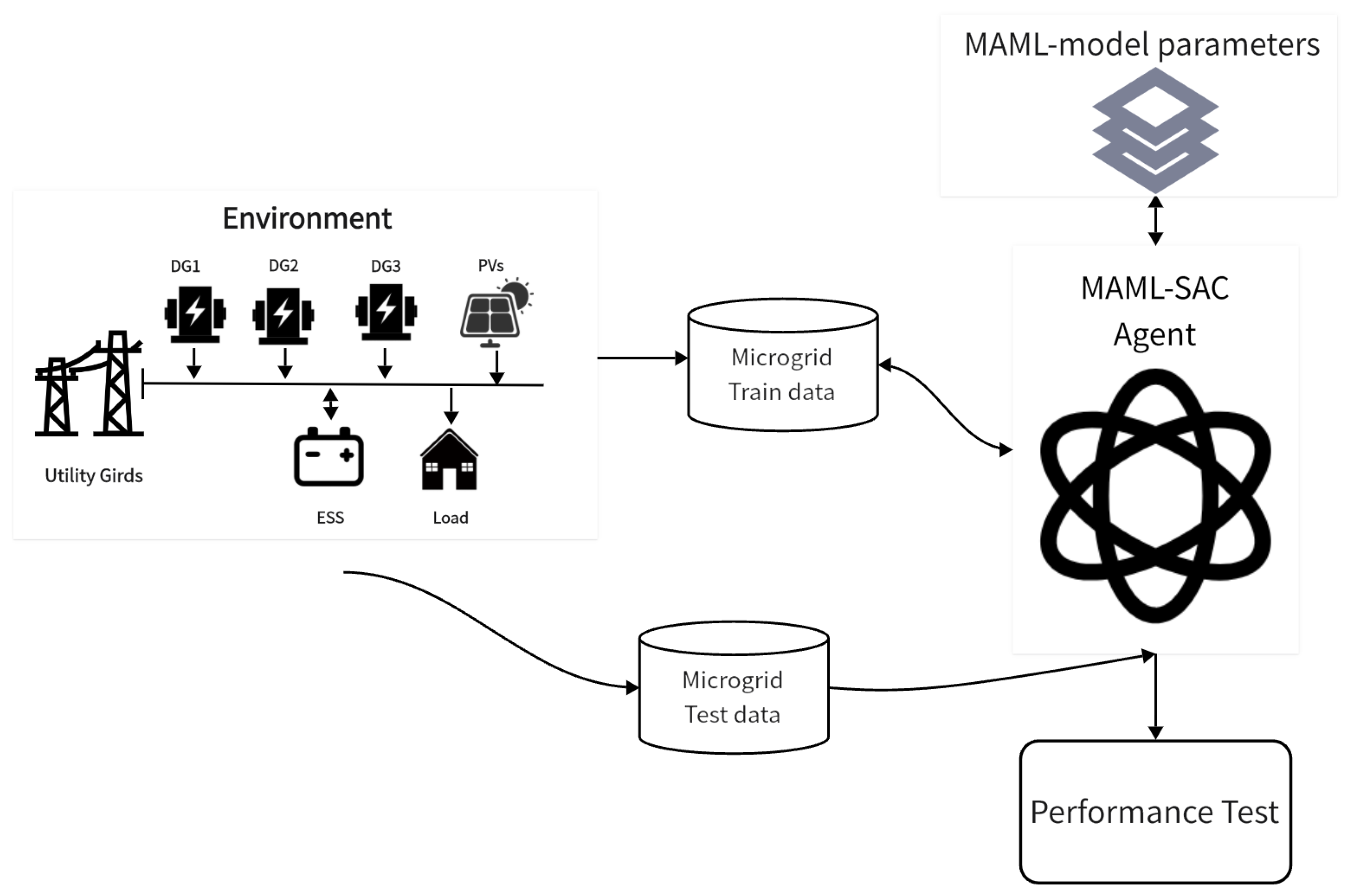
Figure 2 shows the task adaptation phase of the MAML-SAC model. When facing a new microgrid optimization task, the model trained during the meta-learning phase is a starting point for rapid adaptation. By interacting with the new task environment, the model continues to collect data, and these data are used to further fine-tune the model parameters, enabling the model to maximize its adaptability to the specific microgrid configuration. After adapting to the new task, the model’s performance is tested. Based on the test results, the model can be deployed to optimize the operation of the microgrid.

Figure 2.
The task adaptation phase of the MAML-SAC model.
When combining MAML and SAC, the goal is to train a microgrid control policy that can quickly adapt to different operating conditions. The objective function for this approach can be defined as follows:
In the context of the MAML-SAC objective function, N represents the number of tasks, and each task corresponds to a specific microgrid operating scenario. The objective function for task using the SAC algorithm can be defined as:
where r(s, a) is the immediate reward obtained by taking action a in state s. represents the expected value of the value function for the next state s′, where p is the state transition probability. is the entropy regularization term, which encourages exploration in the policy, and is the temperature parameter.
For each task , the policy and value networks are updated through gradient descent. The updated equations can be expressed as follows:
where and are the learning rates for the policy network and the value network, which controls the step size of the gradient descent update for the policy parameters and the value network parameters .
By applying MAML, the model learns parameters and , which enable the policy and value networks to quickly adapt to new microgrid operating tasks with just a few gradient updates. This allows the microgrid control system to efficiently manage and optimize energy resources when faced with different operating conditions and demands.
3.4. Dynamic Learning Rate and Residual Connection
A dynamic learning rate can automatically adjust the learning speed based on the characteristics of different tasks, adopting different learning strategies at different stages and enabling the model to adapt more quickly to new tasks. This is particularly important for rapid adaptability in meta-reinforcement learning. In the later stages of training, reducing the learning rate can reduce the model’s overfitting to training data, thereby improving the model’s generalization ability on new tasks. More importantly, in meta-reinforcement learning, where the model needs to switch between multiple tasks, dynamically adjusting the learning rate can prevent training oscillations caused by excessively large learning rates, maintaining the stability of the training process.
Incorporating residual connections into the meta-reinforcement learning model can help information propagate more effectively through the network, reducing the problem of vanishing gradients during training and accelerating the learning process. This is particularly important in meta-reinforcement learning, as rapid adaptation to new tasks is one of the core goals of meta-learning. Residual connections can also enhance the model’s generalization ability and capacity to represent complex functions, leading to better performance when facing new tasks. This is because residual connections help retain the original input information, allowing the model to better adapt to new environments and tasks. By preserving the input information through the network layers, the model can learn more complex mappings between inputs and outputs, making it more versatile and effective in various microgrid optimization scenarios.
In summary, incorporating residual connections and dynamic learning rates in meta-reinforcement learning can offer several advantages, including accelerating the learning process, improving generalization ability, and preventing training oscillations. These enhancements can make the meta-learning model more effective and efficient in adapting to new tasks and environments, which is crucial for optimizing microgrid operations.
4. Experimental Results
4.1. Experimental Setting
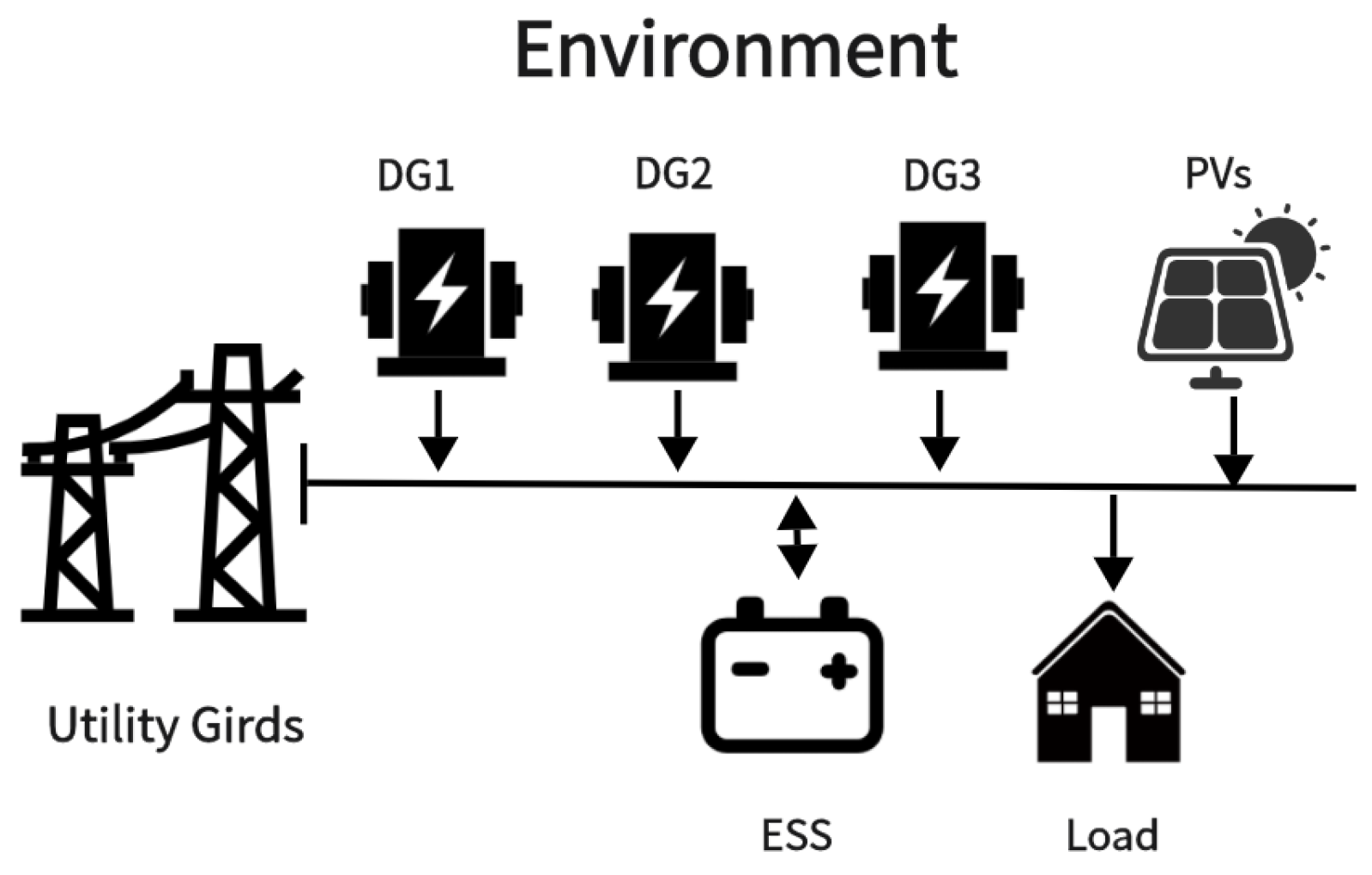
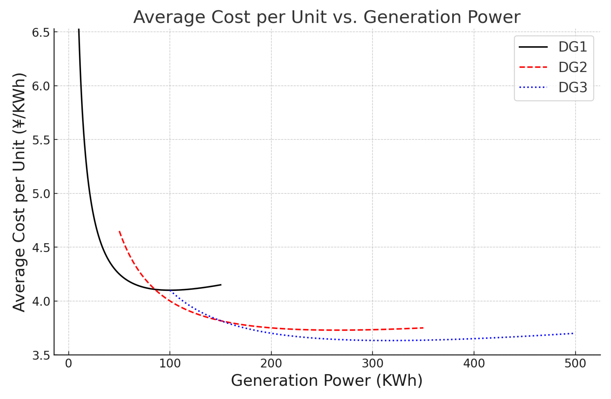
In this section, we evaluate the performance of our proposed framework on the microgrid illustrated in Figure 3. This microgrid is connected to the main grid. It includes three diesel generators (DGs), a photovoltaic (PV) panel, and an Energy Storage System (ESS), which is a battery in this case. The parameters for the three DG units are defined in Table 1. The generation capacity and unit price of each generator are shown in Figure 4. For the ESS, the charge/discharge limits are set to 100 kW, the nominal capacity is set to 500 kW, and the energy efficiency is set to = 0.9. We assume the grid’s maximum export/import limit is 100 kW. To encourage the use of renewable energy, the selling price is set to half the purchase price of electricity, i.e., = 0.5. A data file with hourly resolution is used, including solar power generation, demand consumption, and electricity prices. The raw data in the SAC experiment is divided into training sets and test sets. The training set includes the first three weeks of each month, while the test set contains the remaining data. In the MAML-SAC experiment, the training set consists of data from twenty microgrids different from the one shown in Figure 3, which include variations such as different public grid electricity prices, different numbers and parameters of generators, different load demands, etc. The training data from the SAC experiment is used to fine-tune the MAML-SAC experiment, while the test set remains the same.
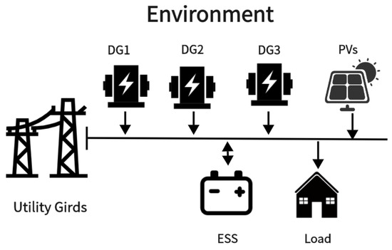
Figure 3.
Microgrid environment in the experiment.

Table 1.
DG unit information.

Figure 4.
The power generation unit price of each generator.
4.2. SAC and MAML-SAC
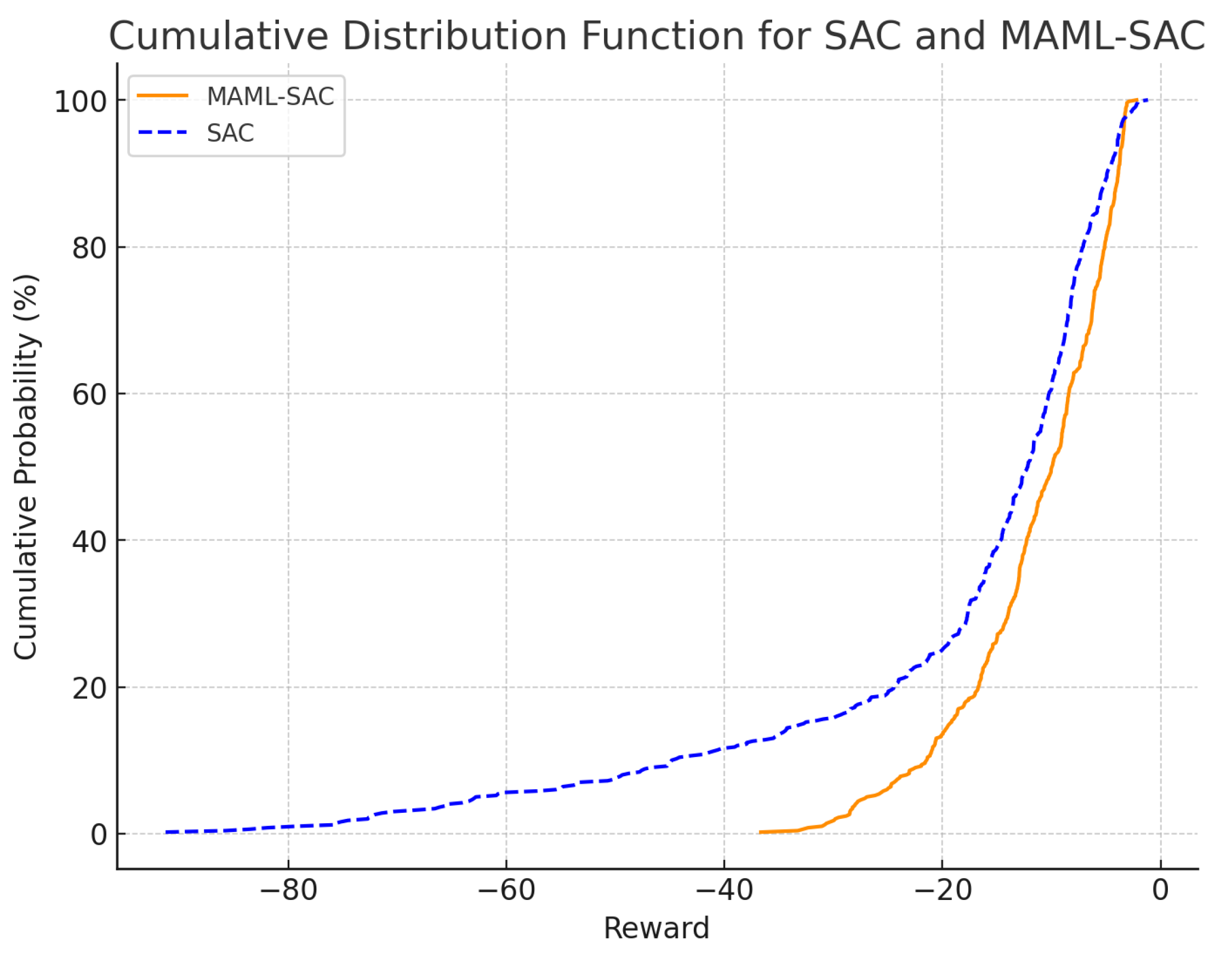
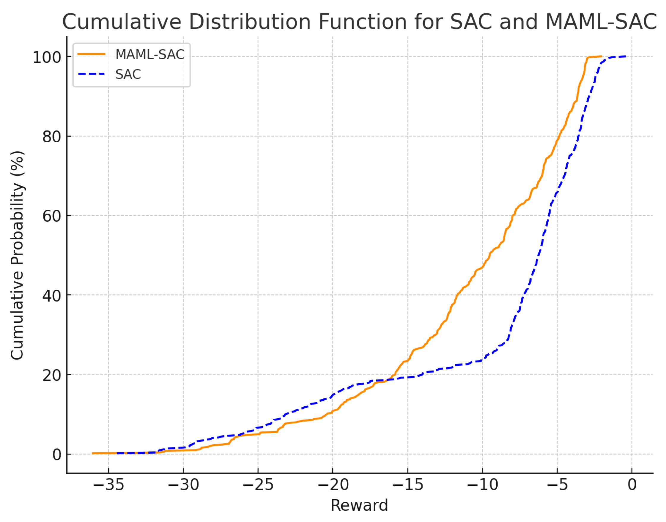
Figure 5 shows the cumulative distribution function (CDF) of rewards for the SAC and MAML-SAC algorithms with one month of training data. In the experimental setup, the reward is inversely proportional to the operational cost of the microgrid: the closer the reward is to zero, the lower the operational cost. The figure indicates that the MAML-SAC method achieves higher rewards than the SAC method, suggesting that MAML-SAC can provide more cost-effective decisions for new microgrid systems with just one month of training data. The SAC method shows that over 10% of the data points have minor rewards, indicating poor performance in some test cases, which could lead to higher operational costs for the microgrid. Figure 6 displays the CDF of rewards for SAC and MAML-SAC with one year of training data. Here, it is evident that SAC performs better with sufficient training data, outperforming the proposed method in about 80% of cases and only underperforming in a minority of cases.
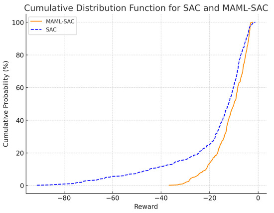
Figure 5.
The CDF of rewards for the SAC and MAML-SAC algorithms with one month of training data.
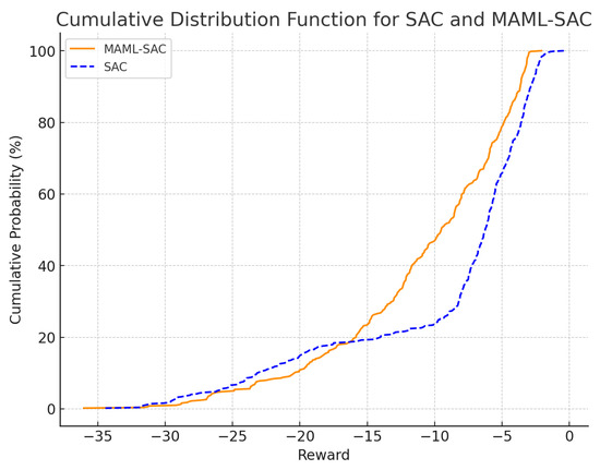
Figure 6.
The CDF of rewards for the SAC and MAML-SAC algorithms with one year of training data.
From the results shown in Figure 5, we can see that the MAML-SAC method proposed in this paper has a significant advantage in quickly adapting to new microgrid environments. This method provides superior decision-making compared to SAC in the early stages of microgrid operation when data is scarce. From the results in Figure 6, it is evident that in situations where there is ample data, RL that trains specifically for a particular microgrid has more advantages. By comparing Figure 5 and Figure 6, we can conclude that in the initial stages of a microgrid’s setup, it is advantageous to use the MAML-SAC approach for decision-making; as data availability increases, switching to the SAC method at an appropriate time can be beneficial. This novel approach maximizes the benefits of microgrids.
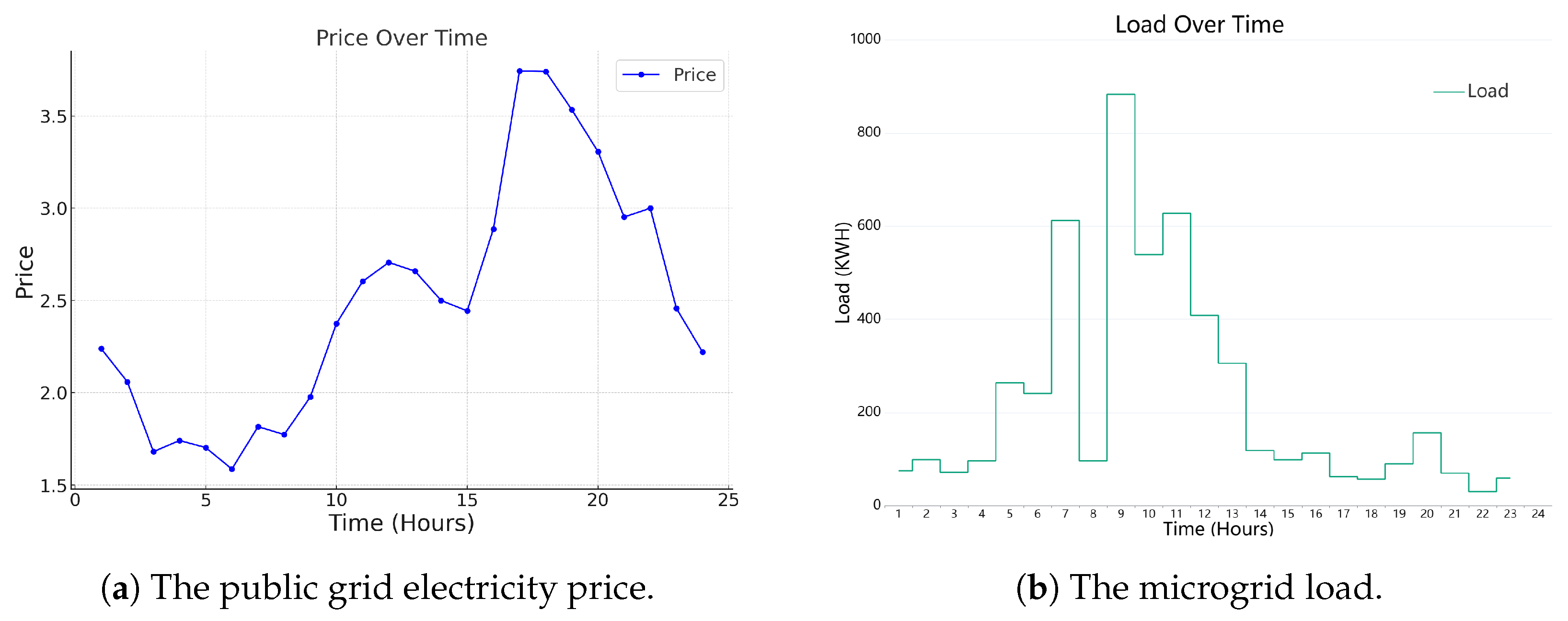
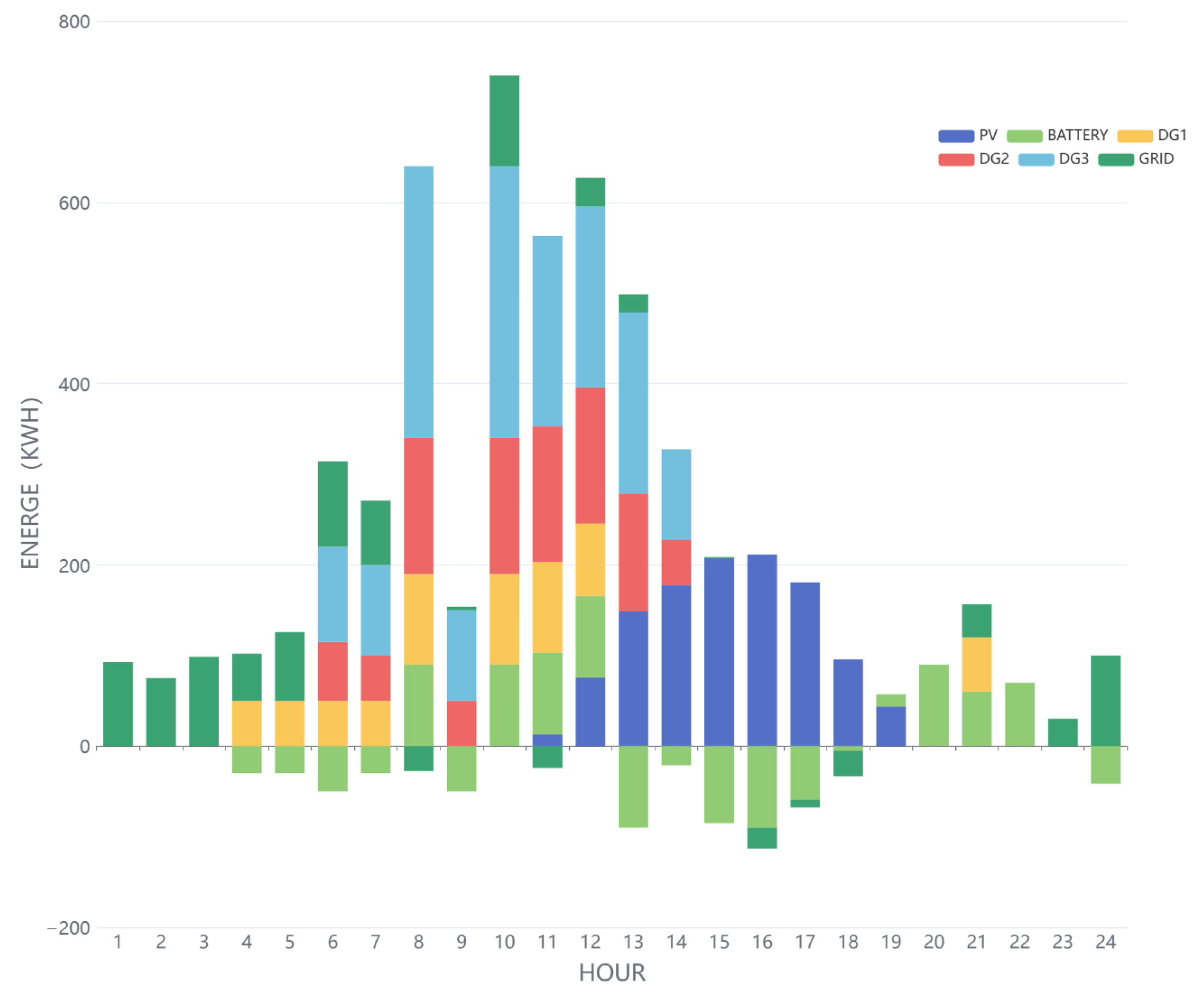
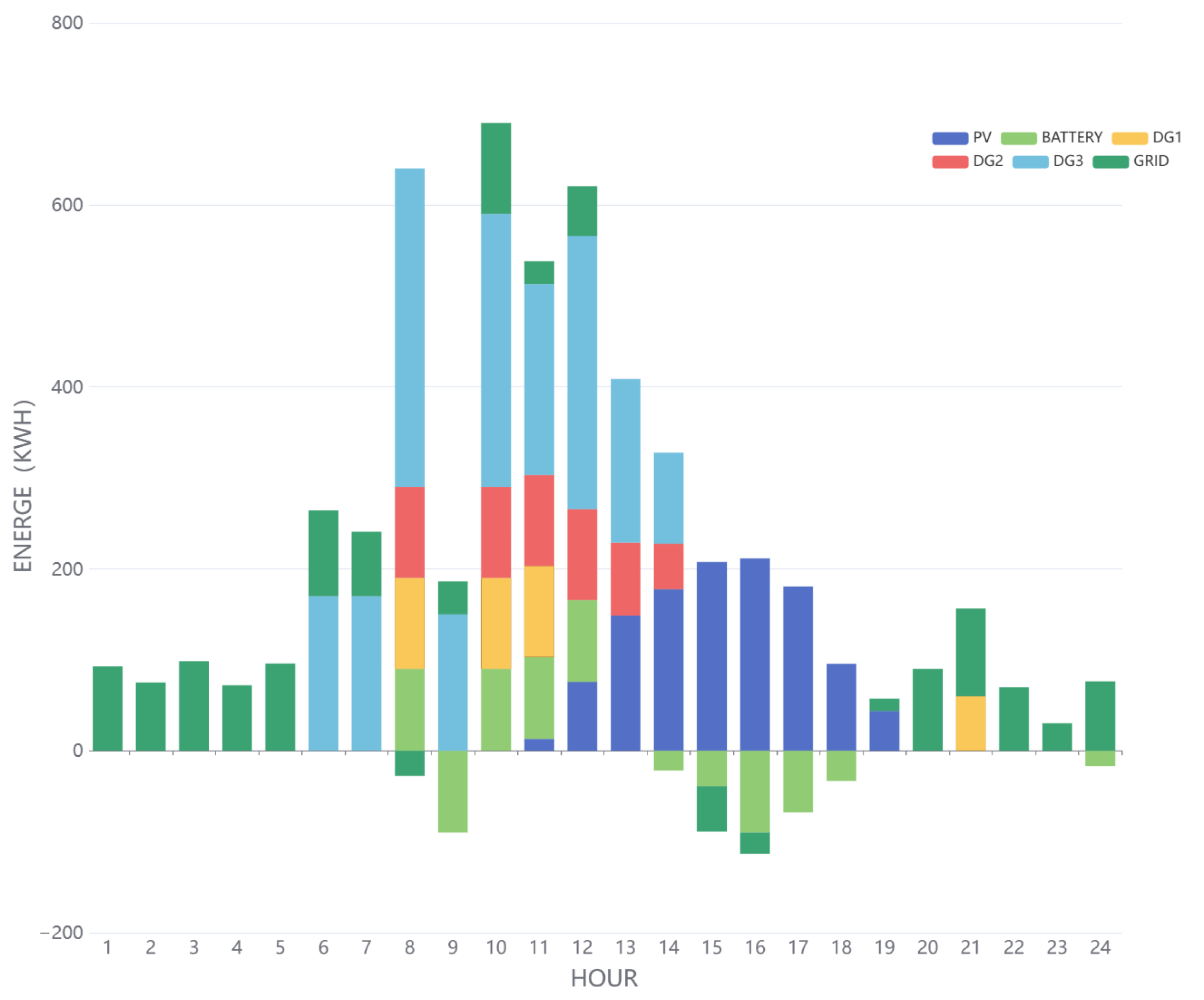
Figure 7 displays hourly data for a specific date, with subfigures (a) and (b) showing the public grid electricity prices and microgrid loads, respectively. Figure 8 and Figure 9 illustrate the charging and discharging states of microgrid components tested on that day after being trained with one month of data using the MAML-SAC and SAC methods, respectively. The above figures indicate that both methods generally meet the load requirements. However, between 9 a.m. and 10 p.m., when there is a sudden surge in load, the microgrid components struggle to provide sufficient power due to power output limitations and generator ramping restrictions, with the SAC method exhibiting more significant load shedding. Furthermore, MAML-SAC demonstrates its sensitivity and adaptability to economic efficiency by discharging the battery during high electricity price periods and preemptively storing energy during low-price periods. On the other hand, SAC, possibly due to a lack of training data, may not have understood the trends in electricity prices and load changes and, therefore, failed to store energy during low-price periods. Overall, the method proposed in this paper can quickly adapt to new microgrids under conditions of scarce data and make excellent decisions, optimizing energy efficiency and cost-effectiveness. The responsiveness of the MAML-SAC algorithm to fluctuations in electricity prices and load demands showcases its high adaptability and foresight in decision-making, proving its potential in effectively managing microgrid operations.
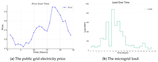
Figure 7.
The hourly data of a specific day.
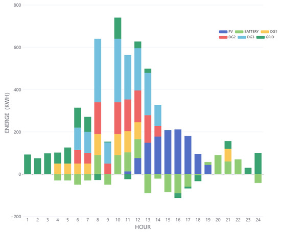
Figure 8.
The charging/discharging status of microgrid components during the MAML-SAC test.

Figure 9.
The charging/discharging status of microgrid components during the SAC test.
5. Discussion and Conclusions
This paper proposes a real-time energy scheduling strategy for microgrids based on meta-reinforcement learning, which fully utilizes the advantages of combining meta-learning and RL to make excellent decisions in microgrid systems with only a small amount of training data. The experimental results show that the algorithm proposed in this paper exhibits better performance compared to RL algorithms at the initial stage of microgrid operation when data are scarce. However, this method still has some shortcomings, such as its performance not being as good as RL when data are abundant. There is excellent potential for further exploration in combining various RL and meta-learning approaches for microgrid optimization. As the field advances, more advanced algorithms can be developed to enhance microgrid systems’ adaptability, efficiency, and robustness. Continued research in this area can lead to more intelligent and autonomous energy management solutions, which are crucial for the sustainable and reliable operation of microgrids in the future.
Author Contributions
Conceptualization, X.S.; methodology, H.S.; software, H.S.; validation, H.S. and Y.C.; data curation, H.S. and Y.C.; writing—original draft preparation, H.S.; writing—review and editing, X.S. All authors have read and agreed to the published version of the manuscript.
Funding
This work was supported by the Pioneer and Leading Goose R&D Program of Zhejiang (Grant No. 2023C01143), the National Natural Science Foundation of China (Grant No. 62072121), and the Zhejiang Provincial Natural Science Foundation (Grant No. LLSSZ24F020001).
Data Availability Statement
The original contributions presented in the study are included in the article, further inquiries can be directed to the corresponding author.
Conflicts of Interest
The authors declare no conflicts of interest.
List of Symbols
| The total operating cost | |
| The costs exchanged in buying from and selling to the main grid | |
| Generation cost | |
| The cost of load shedding | |
| The energy stored in the ESS | |
| Maximum and minimum allowable energy level | |
| The power exchanged in buying from and selling to the main grid | |
| Charging and discharging powers | |
| Maximum allowable charging and discharging powers | |
| Generator’s power output | |
| The upper and lower limits of the generator’s power output | |
| Maximum exchange power with the main grid | |
| The total load | |
| The power of load shedding | |
| The ramping up and ramping down capabilities of the DG units |
References
- Li, L.; Lin, J.; Wu, N.; Xie, S.; Meng, C.; Zheng, Y.; Wang, X.; Zhao, Y. Review and outlook on the international renewable energy development. Energy Built Environ. 2022, 3, 139–157. [Google Scholar] [CrossRef]
- Kung, C.C.; McCarl, B.A. Sustainable energy development under climate change. Sustainability 2018, 10, 3269. [Google Scholar] [CrossRef]
- Ray, P. Renewable energy and sustainability. Clean Technol. Environ. Policy 2019, 21, 1517–1533. [Google Scholar] [CrossRef]
- Lund, H. Renewable energy strategies for sustainable development. Energy 2007, 32, 912–919. [Google Scholar] [CrossRef]
- Mahmoud, M.S.; Hussain, S.A.; Abido, M.A. Modeling and control of microgrid: An overview. J. Frankl. Inst. 2014, 351, 2822–2859. [Google Scholar] [CrossRef]
- Lasseter, R.; Akhil, A.; Marnay, C.; Stephens, J.; Dagle, J.; Guttromsom, R.; Meliopoulous, A.S.; Yinger, R.; Eto, J. Integration of Distributed Energy Resources. The CERTS Microgrid Concept; Technical Report; Lawrence Berkeley National Lab. (LBNL): Berkeley, CA, USA, 2002. [Google Scholar]
- Zia, M.F.; Elbouchikhi, E.; Benbouzid, M. Microgrids energy management systems: A critical review on methods, solutions, and prospects. Appl. Energy 2018, 222, 1033–1055. [Google Scholar] [CrossRef]
- Shi, W.; Xie, X.; Chu, C.C.; Gadh, R. Distributed optimal energy management in microgrids. IEEE Trans. Smart Grid 2014, 6, 1137–1146. [Google Scholar] [CrossRef]
- Kou, P.; Liang, D.; Gao, L. Stochastic energy scheduling in microgrids considering the uncertainties in both supply and demand. IEEE Syst. J. 2016, 12, 2589–2600. [Google Scholar] [CrossRef]
- Hussain, A.; Bui, V.H.; Kim, H.M. Robust optimization-based scheduling of multi-microgrids considering uncertainties. Energies 2016, 9, 278. [Google Scholar] [CrossRef]
- Dimeas, A.L.; Hatziargyriou, N.D. Operation of a multiagent system for microgrid control. IEEE Trans. Power Syst. 2005, 20, 1447–1455. [Google Scholar] [CrossRef]
- Logenthiran, T.; Srinivasan, D.; Wong, D. Multi-agent coordination for DER in MicroGrid. In Proceedings of the 2008 IEEE International Conference on Sustainable Energy Technologies, Singapore, 24–27 November 2008; IEEE: Piscataway, NJ, USA, 2008; pp. 77–82. [Google Scholar]
- Li, W.; Logenthiran, T.; Woo, W.L. Intelligent multi-agent system for smart home energy management. In Proceedings of the 2015 IEEE Innovative Smart Grid Technologies-Asia (ISGT ASIA), Bangkok, Thailand, 3–6 November 2015; IEEE: Piscataway, NJ, USA, 2015; pp. 1–6. [Google Scholar]
- Lasseter, R.H.; Paigi, P. Microgrid: A conceptual solution. In Proceedings of the 2004 IEEE 35th Annual Power Electronics Specialists Conference (IEEE Cat. No. 04CH37551), Aachen, Germany, 20–25 June 2004; IEEE: Piscataway, NJ, USA, 2004; Volume 6, pp. 4285–4290. [Google Scholar]
- Zhu, B.; Xia, X. Adaptive model predictive control for unconstrained discrete-time linear systems with parametric uncertainties. IEEE Trans. Autom. Control 2015, 61, 3171–3176. [Google Scholar] [CrossRef]
- Molderink, A.; Bakker, V.; Bosman, M.G.; Hurink, J.L.; Smit, G.J. Management and control of domestic smart grid technology. IEEE Trans. Smart Grid 2010, 1, 109–119. [Google Scholar] [CrossRef]
- Parisio, A.; Rikos, E.; Glielmo, L. A model predictive control approach to microgrid operation optimization. IEEE Trans. Control Syst. Technol. 2014, 22, 1813–1827. [Google Scholar] [CrossRef]
- Garcia-Torres, F.; Zafra-Cabeza, A.; Silva, C.; Grieu, S.; Darure, T.; Estanqueiro, A. Model predictive control for microgrid functionalities: Review and future challenges. Energies 2021, 14, 1296. [Google Scholar] [CrossRef]
- Kaelbling, L.P.; Littman, M.L.; Moore, A.W. Reinforcement learning: A survey. J. Artif. Intell. Res. 1996, 4, 237–285. [Google Scholar] [CrossRef]
- Mnih, V.; Kavukcuoglu, K.; Silver, D.; Rusu, A.A.; Veness, J.; Bellemare, M.G.; Graves, A.; Riedmiller, M.; Fidjeland, A.K.; Ostrovski, G.; et al. Human-level control through deep reinforcement learning. Nature 2015, 518, 529–533. [Google Scholar] [CrossRef] [PubMed]
- Kiran, B.R.; Sobh, I.; Talpaert, V.; Mannion, P.; Al Sallab, A.A.; Yogamani, S.; Pérez, P. Deep reinforcement learning for autonomous driving: A survey. IEEE Trans. Intell. Transp. Syst. 2021, 23, 4909–4926. [Google Scholar] [CrossRef]
- Sallab, A.E.; Abdou, M.; Perot, E.; Yogamani, S. Deep reinforcement learning framework for autonomous driving. arXiv 2017, arXiv:1704.02532. [Google Scholar]
- Ebert, F.; Finn, C.; Dasari, S.; Xie, A.; Lee, A.; Levine, S. Visual foresight: Model-based deep reinforcement learning for vision-based robotic control. arXiv 2018, arXiv:1812.00568. [Google Scholar]
- Lample, G.; Chaplot, D.S. Playing FPS games with deep reinforcement learning. In Proceedings of the AAAI Conference on Artificial Intelligence, San Francisco, CA, USA, 4–9 February 2017; Volume 31. [Google Scholar]
- Bui, V.H.; Hussain, A.; Kim, H.M. Q-learning-based operation strategy for community battery energy storage system (CBESS) in microgrid system. Energies 2019, 12, 1789. [Google Scholar] [CrossRef]
- Alabdullah, M.H.; Abido, M.A. Microgrid energy management using deep Q-network reinforcement learning. Alex. Eng. J. 2022, 61, 9069–9078. [Google Scholar] [CrossRef]
- Mu, C.; Shi, Y.; Xu, N.; Wang, X.; Tang, Z.; Jia, H.; Geng, H. Multi-Objective Interval Optimization Dispatch of Microgrid via Deep Reinforcement Learning. IEEE Trans. Smart Grid 2023, 15, 2957–2970. [Google Scholar] [CrossRef]
- Hospedales, T.; Antoniou, A.; Micaelli, P.; Storkey, A. Meta-learning in neural networks: A survey. IEEE Trans. Pattern Anal. Mach. Intell. 2021, 44, 5149–5169. [Google Scholar] [CrossRef] [PubMed]
- Rihan, S.D.A.; Anbar, M.; Alabsi, B.A. Meta-Learner-Based Approach for Detecting Attacks on Internet of Things Networks. Sensors 2023, 23, 8191. [Google Scholar] [CrossRef] [PubMed]
- Gao, D.; He, X.; Zhou, Z.; Tong, Y.; Thiele, L. Pruning meta-trained networks for on-device adaptation. In Proceedings of the 30th ACM International Conference on Information & Knowledge Management, Virtual Event, 1–5 November 2021; pp. 514–523. [Google Scholar]
- Nooralahzadeh, F.; Bekoulis, G.; Bjerva, J.; Augenstein, I. Zero-shot cross-lingual transfer with meta learning. arXiv 2020, arXiv:2003.02739. [Google Scholar]
- Zhu, Y.; Liu, C.; Jiang, S. Multi-attention Meta Learning for Few-shot Fine-grained Image Recognition. In Proceedings of the Twenty-Ninth International Joint Conference on Artificial Intelligence (IJCAI), Yokohama, Japan, 11–17 July 2020; pp. 1090–1096. [Google Scholar]
- Deng, Q.; Zhao, Y.; Li, R.; Hu, Q.; Liu, T.; Li, R. Context-Enhanced Meta-Reinforcement Learning with Data-Reused Adaptation for Urban Autonomous Driving. In Proceedings of the 2023 International Joint Conference on Neural Networks (IJCNN), Gold Coast, Australia, 18–23 June 2023; IEEE: Piscataway, NJ, USA, 2023; pp. 1–8. [Google Scholar]
- Gao, S.; Xiang, C.; Yu, M.; Tan, K.T.; Lee, T.H. Online optimal power scheduling of a microgrid via imitation learning. IEEE Trans. Smart Grid 2021, 13, 861–876. [Google Scholar] [CrossRef]
Disclaimer/Publisher’s Note: The statements, opinions and data contained in all publications are solely those of the individual author(s) and contributor(s) and not of MDPI and/or the editor(s). MDPI and/or the editor(s) disclaim responsibility for any injury to people or property resulting from any ideas, methods, instructions or products referred to in the content. |
© 2024 by the authors. Licensee MDPI, Basel, Switzerland. This article is an open access article distributed under the terms and conditions of the Creative Commons Attribution (CC BY) license (https://creativecommons.org/licenses/by/4.0/).