
Simulation and Experimental Verification of Dispersion and Explosion of Hydrogen–Methane Mixture in a Domestic Kitchen †

1
Weifang Municipal Public Utility Service Center, 332 Kangdong Street, Kuiwen District, Weifang 261000, China
2
School of Civil Engineering, Chongqing University, 174 Shazheng Street, Shapingba District, Chongqing 400044, China
3
WISDRI City Environment Protection Engineering Co., Ltd., No. 59 Liufang Road, East Lake Hi-Tech Development Zone, Wuhan 430200, China
4
National Center of Technology Innovation for Fuel Cell, 169 Wei’an Road, High-Tech Zone, Weifang 261000, China
*
Author to whom correspondence should be addressed.
†
This paper is an extended version of our paper published in the 19th International Conference on Sustainable Energy Technologies, Istanbul, Turkey, 16–18 August 2022; pp. 301–310.
Energies 2024, 17(10), 2320; https://doi.org/10.3390/en17102320
Submission received: 9 April 2024
/
Revised: 5 May 2024
/
Accepted: 8 May 2024
/
Published: 11 May 2024
(This article belongs to the Special Issue Hydrogen Safety for Energy Applications)
Abstract
:Hydrogen is a carbon-free energy source that can be obtained from various sources. The blending of hydrogen represents a transitional phase in the shift from natural gas systems to hydrogen-based systems. However, concerns about the safety implications of introducing hydrogen have led to extensive discussions. This paper utilizes Fluent 17.0 numerical simulation software to simulate the leakage of hydrogen-blended natural gas in a closed domestic kitchen and analyze the concentration distribution and its variation pattern after a leakage. An experimental platform is set up, and a mixture of nitrogen and helium gas is used as a substitute for hydrogen-blended natural gas for the simulations and experiments. The simulation results demonstrate that the leaked gas spreads and accumulates towards the top of the space, gradually filling the entire area as the leak persists. As the hydrogen content in the leaked gas increases, the dispersion capacity of the gas in the confined space also increases. Furthermore, as the flow rate of the leaked gas increases, the average concentration of the leaked gas rises, and the gas stratification in the confined kitchen diminishes. The concentration distribution observed in the experiments aligns with the simulation results. After establishing the feasibility conditions of the model, the dispersion of the hydrogen-blended natural gas in the kitchen is further simulated. The results suggest that blending hydrogen into the gas enhances the dispersion of the gas after a leak, leading to a wider distribution within the kitchen and an increased risk in the event of a leak. Additionally, this paper employs the CASD module of FLACS 11.0 software to construct a three-dimensional geometric model of the domestic kitchen for simulation studies on the explosion of hydrogen-blended natural gas in a confined space. By adjusting the hydrogen ratio in the combustible gases present in the space and examining the variations in hydrogen concentration and external conditions, such as opening or closing the door, the influence on parameters including the peak explosion pressure, explosion overpressure, explosion flame temperature, and explosion response time are examined. Furthermore, the extent of the explosion area is determined, and the effect of hydrogen on the blast is clarified.
1. Introduction
Blending hydrogen with natural gas is a growing trend in the green development of natural gas. This blending has the potential to significantly reduce the carbon emissions associated with natural gas. However, it is important to note that hydrogen and methane, the main components of natural gas, have distinct physical and chemical properties. For example, hydrogen has a higher diffusion coefficient and can spread more rapidly if it leaks under the same conditions. Additionally, hydrogen has wider explosion limits compared to natural gas, which introduces increased risks to the natural gas pipeline network when blended together.
Numerical simulations have been conducted widely to study the dispersion of combustible gas leaks in various spaces. Simulations of the low-rate leakage and dispersion of hydrogen–helium gas mixtures in confined spaces have revealed that the size of the leak aperture has a negligible effect on the concentration at the monitoring point. However, the location of the leak, mass leak rate, and duration of the leak significantly impact the concentration [1]. An experimental study comparing the distribution of hydrogen and helium has demonstrated that helium can serve as a reliable proxy for similarity when studying plume release [2]. The dispersion behavior of the remaining gas after a leak can be examined through the study of hydrogen leaks in closed cylinder chambers. It has been concluded that the risk increases as the leak height rises [3]. Simulations of the consequences of accidental hydrogen leaks in warehouses larger than 15,000 m have shown that the peak pressure resulting from hydrogen ignition varies significantly depending on the release rate, warehouse volume, and presence of a ventilation system [4]. The roof angle in a garage affects the leakage, with a lower hydrogen concentration observed at a roof angle of 120° [5]. In the case of hydrogen leaks from fuel cell vehicles (FCVs) in underground parking lots, where the volume of the combustible zone grows non-linearly with time and experiences a latent period, the use of ventilators can effectively prevent the dangerous situation of hydrogen leakage [6]. Experimental results on the build-up behavior of hydrogen-blended natural gas leaks in residential housing have indicated that blending the gas with hydrogen increases the leak rate at the same leak pressure [7]. Studies on the dispersion stratification of hydrogen and natural gas mixtures have revealed that there is concentration stratification during a leak, which diminishes over time after the leak has ceased. No separation of hydrogen from natural gas is observed in any of the studied scenarios [8]. The layout of the building environment significantly influences gas leakage and dispersion patterns, with a closed layout offering the highest level of wind blockage, the most pronounced vortex effect, and the widest range of high gas concentrations [9].
Simulations of combustible gas explosions can be conducted using FLACS software. Research has been performed on three different scenarios: garages, large car parks, and tunnels. These studies have shown that the explosive intensity of methane and hydrogen gas mixtures is much stronger than that of methane alone. However, the resulting explosion overpressure is lower when methane is mixed with hydrogen compared to pure hydrogen gas [10]. In a residential setting, some researchers have proposed a quantitative risk assessment method for gas leakage explosions. This method involves analyzing gas dispersion and establishing an explosion simulation model to predict the consequences of an explosion in an inhomogeneous gas cloud. Quantitatively describing the severity of the consequences of the explosion in different areas of a residence helps identify hazardous areas [11]. Using FLACS software, a simulation was conducted in a 200 m long tunnel to study the overpressure distribution and flame changes resulting from the explosion of a methane–hydrogen gas mixture. The simulation results revealed that the overpressure generated by a mixture of 10–20% hydrogen and natural gas increased by 16–32%. This indicates that the addition of hydrogen increases the risk of a natural gas explosion. The quality of the leaked gas did not have a significant impact on the explosion overpressure, while the shape of the vapor cloud, particularly its height, had a more pronounced effect [12]. In a study on accidental explosions, a consistent physical model was established. Explosion simulation software was used to simulate a gas explosion based on the volume and range of the accidental leakage. The propagation process of the shock wave in a building was analyzed, and shock wave curves were drawn at different locations. The numerical simulation results were then compared to actual accident data. The simulation results aligned well with the observed damage, thus confirming the effectiveness of the software [13]. Researchers conducted experiments in a rectangular closed space measuring 18 m × 3 m × 3 m to investigate the explosion characteristics of methane–hydrogen mixtures. The aim was to vary the obstacles and the methane–hydrogen ratio in order to determine the impact on explosions. The results showed that when the hydrogen content exceeded 20%, the shockwave generated from the explosion was significantly larger compared to that with pure methane, indicating a potential risk of deflagration. Additionally, reducing obstacles in the closed space decreased the risk of deflagration and overpressure [14]. In another experiment, diffusion layering experiments were conducted on methane–hydrogen mixtures in a larger facility with a closed space volume of 25 cubic meters, which is equivalent to the size of a room or garage. These experiments revealed that the gas mixture within the space exhibited inhomogeneity under both ventilated and non-ventilated conditions [8]. Furthermore, in a laboratory setting resembling a household room, experiments were carried out to study the diffusion of methane and hydrogen mixtures. The variables included the mixture ratio, leak diameter, leak height, and the position of ventilation openings. Increasing the percentage of hydrogen in the mixture resulted in a higher volume flow rate of the leaked gas mixture, leading to greater gas concentrations and larger gas accumulation areas. However, the increase in the hydrogen content also enhanced buoyancy, resulting in increased airflow through ventilation openings. As a result, the rise in the hydrogen concentration had a relatively smaller effect on the concentration increase, but it led to higher overall concentrations. Moreover, due to the wider flammability range, the presence of a combustible volume also increased over time [7].
With the growing popularity and advancement of numerical simulation software, an increasing number of researchers are employing this technology to investigate the propagation and repercussions of leaks. Nevertheless, it is essential to take into account the reliability of numerical simulations, as there are numerous factors that can influence results under real-world operating conditions. Furthermore, previous studies have primarily concentrated on analyzing a single gas, such as natural gas or hydrogen exclusively. Given the current energy trends and the practical operating environment of natural gas pipelines, it is imperative to explore the dispersion of hydrogen-blended natural gas leaks and the potential consequences of flammable gas leaks and explosions in confined spaces.
The primary objective of this paper is to investigate the occurrence of leaks and explosions caused by hydrogen-blended natural gas in domestic kitchens. Numerical simulation methods are employed to validate the accuracy of the chosen approach through experimental testing. The findings of this study aim to support the subsequent analysis of the repercussions of hydrogen-blended natural gas leaks and encourage the adoption of green gas and the utilization of hydrogen-blended natural gas in the future.
2. Materials and Methods
2.1. Numerical Simulation
2.1.1. Leakage Mathematical Model
The volume flow of leakage after a pipeline failure primarily depends on factors such as orifice size and pressure. The leakage volume of the experiment and simulation can be calculated using the natural gas leakage diffusion model. There are several commonly used models for natural gas leakage, including the small-bore leak model, the pipe leak model, and the integrated pipe–small bore model for any size of leakage. Figure 1 is a schematic diagram of the small-bore leak model.
- The small-bore leak model:
When ,
When ,
- The pipeline leakage model:
—critical pressure ratio;
—leakage mass flow, kg/s;
—the mass flow rate of gas in the upstream pipeline of the leakage point, kg/s;
—flow coefficient; can be taken as 0.9~0.98;
—equivalent diameter of the leak orifice, m;
—environmental pressure, Pa;
—absolute pressure at point 1, Pa;
—absolute pressure at point 2, Pa;
—the gas constant of a certain type of gas, J/(kg·K);
—gas temperature at point 1, K;
—gas temperature at point 2, K;
—the isentropic index of gas;
—polytropic index;
—inner diameter of pipeline, m;
—friction resistance coefficient;
—the distance from the leakage point to the starting point of the pipeline, m.
- The integrated pipe–small bore model:When a small hole develops a leak, the resistance to gas flow along the pipeline causes the pressure at the leak to be lower than the initial pressure of the pipeline. If we assume that all the gas in the pipeline flows out through the leak and there is no flow downstream of the leak, then the pressure at the leak will be at its highest and the flow rate of the leak will also be at its highest. Therefore,By combining the above four formulas and inputting the data for calculation, we can obtain the relevant parameters required for all sizes of leakage.
In this paper, we will select the appropriate calculation model based on the specific conditions of the experiment and simulation. By inputting the relevant parameters of the gas at different blending ratios into the algorithm, we can calculate the leakage flow rate of the hydrogen-blended gas. The experiment and simulations will then be conducted based on the calculated results.
2.1.2. Numerical Simulation Models
Based on the actual construction of the experimental kitchen, a conventional size model measuring 2.5 m × 1.6 m × 2.6 m was built using the ANSYS 17.0 pre-processing software ICEM. The geometric model was simulated to incorporate the necessary detectors and shelves for the experiment. Simultaneously, the airflow resulting from gas leaks during the experiment was simulated to account for disturbances. The domestic kitchen includes a worktop, door, window, wall, range hood, and leak point. The leak point, located on the cooktop below the range hood, is a circular hole with a diameter of 8 mm. Refer to Figure 2 for the specific geometric model.
To combine simulation and experiment, nine detectors were installed in the kitchen and distributed across four horizontal surfaces. Oxygen concentration monitoring points were placed at these detection points to observe changes in oxygen concentration during the leak simulation. The locations of the oxygen concentration monitoring points in the numerical simulation are displayed in Figure 3.
During the explosion simulation, the simulation area of the external space of the kitchen was expanded based on the physical model of the kitchen. Refer to Figure 4 for the explosion simulation model.
Detectors were also positioned inside the kitchen, as well as outside the doors and windows. The locations of the detection points can be seen in Figure 5.
2.1.3. Numerical simulation parameter setting
- 1.
- Leakage dispersion numerical simulation.
The pressure-based solver is selected for mesh division and monitoring point setting. The transient calculation mode needs to be set for the simulated leakage process.
The basic control equation of Fluent is as follows:
- Continuity equation:
The density of incompressible fluids is constant, so,
—the velocity components in the x, y, and z directions, m/s;
—time, s;
—density, kg/m3.
- Momentum equation:
x direction:
y direction:
z direction:
—the velocity components in the x, y, and z directions, m/s;
—turbulent viscosity of fluids, Pa·s.
- Energy equation:
—temperature, K;
—turbulent thermal conductivity, W/m·K;
—constant, usually taken from 0.9 to 1;
—the specific heat at constant pressure for the leaking fluid, air, and mixture fluid, , J/(kg·K);
- Density equation:
—universal gas constant, J/(mol·K);
—absolute pressure, Pa;
—average molecular weight of the gas mixture, kg/mol;
—the molecular weight of air, kg/mol;
—molecular weight of leaked and diffused substances, kg/mol;
—mass fraction of components;
- Composition equation:
—turbulent diffusion coefficient, m2/s.
The ICEM (ANSYS 17.0) software is used to divide the non-structural mesh of the kitchen geometry model. Different meshing parameters are set for structures of different sizes and flow field strengths in the kitchen. The model’s mesh independence is verified before performing the simulation. The number of meshes used for the simulation is 53 w, 86 w, 139 w, 156 w, and 188 w. The minimum number of meshes required to meet the calculation accuracy requirements is 139 w. The mesh division diagram is shown in Figure 6.
The location coordinates of the nine monitoring points in the model are as follows: point 1 (0.50, 1.55, 2.05), point 2 (1.53, 0.05, 2.05), point 3 (0.76, 0.96, 1.68), point 4 (2.32, 0.96, 1.68), point 5 (1.50, 0.50, 1.68), point 6 (0.76, 0.50, 1.15), point 7 (1.50, 0.96, 1.15), point 8 (2.32, 0.50, 1.15), and point 9 (1.50, 0.50, 0.20). The volumetric concentration fractions of oxygen at these nine monitoring points were selected as indicator to facilitate comparison with experimental data. Since the trend and magnitude of oxygen concentration changes derived from detectors located in the same plane were essentially the same, the results were analyzed by selecting one detector point from each of the four planes to represent the oxygen concentration changes in that plane. Detector 1 was selected for the highest plane z = 2.05 m, detector 5 for plane z = 1.68 m, detector 8 for plane z = 1.15 m, and only detector 9 for the lowest plane z = 0.2 m.
The operating table and the wall are always set as wall boundary conditions in the boundary condition settings. The leak point is set as a velocity inlet. A small gap in the window is opened and set as a pressure outlet to maintain the balance of the simulation process. The velocity and flow rate at the leak point are calculated using actual data. As the percentage of hydrogen blending increases, the mass flow rate of the gas decreases and the leak rate increases. Doors and windows are set as wall boundary conditions. The simulation verified that an open cooker hood would rapidly dilute the combustible gas in the kitchen, resulting in no explosive area. Therefore, the study was carried out with the cooker hood closed as a wall boundary condition. Table 1 shows the setting of boundary conditions.
In the gas parameter settings, pure nitrogen, pure helium, and a nitrogen–helium mixture (20%vol of helium) were used for numerical simulations of leak dispersion in the domestic kitchen, with leakage flow rates set at 4 Nm3, 8 Nm3, and 12 Nm3, respectively. For the numerical simulation of hydrogen-blended natural gas, we calculated the leakage flow rate and leakage rate under actual working conditions using basic parameters such as gas density and friction resistance coefficient. These calculations were based on three natural gas leakage models. Table 2 displays the leakage flow rate and leakage rate for various hydrogen blending ratios.
Table 3 displays various properties of the gases utilized in experiments and simulations.
- 2.
- Explosion numerical simulation.
FLACS still adheres to the three conservation laws while simulating the explosion process, as represented by Formulas (5)–(10). The explosion process follows the law of fluid chemical reactions, as follows:
- Dalton’s theorem for ideal gases:
—the gas pressure, Pa;
—the pressure of each component gas, Pa;
—the volume of gas, m3.
- Isentropic ratio:
—specific heat at constant pressure, J/(kg·K);
—specific heat at constant volume, J/(kg·K).
- Pressure–density–temperature relationship:
—density, kg/m3;
—the temperature of the flow field, K.
- By employing the finite volume method and applying the appropriate boundary conditions, the N-S equation can be solved accurately. This enables us to determine the variations in key parameters within the relevant region, including temperature, overpressure value, flame velocity, combustion products, and combustion material consumption:
—universal variable;
—time, s;
—the horizontal coordinate position of the fluid along the j direction, m;
—the velocity vector in the j direction, m/s;
—the diffusion coefficient, m2/s;
—source term.
FLACS utilizes the k-ε two-equation model and standard wall functions to simulate turbulence. The k-ε model consists of two additional transport equations.
- The turbulent pulsation kinetic energy k is
- Turbulent pulsation kinetic energy dissipation rate ε for
—molecular viscosity of fluids, Pa·s;
—turbulent viscosity of fluids, Pa·s;
and —Prandtl numbers corresponding to k and ε, usually taken as 1 and 1.3;
—the generation term of turbulent kinetic energy caused by the average velocity gradient;
—the generation term of turbulent kinetic energy caused by buoyancy;
—the contribution of pulsatile expansion;
, , and —constants, usually taken as 1.44, 1.92, and 0.09;
and —source term.
The FLACS pre-processor CASD was used to construct the geometrical model, and the computational domain was established based on the dimensions of the model. A series of simulation tests were conducted to determine the optimal mesh resolution, with 0.05 m yielding the most reliable results. This resolution was consequently applied throughout the study, with a uniform mesh created across the entire computational area. The number of meshes in the three directions was set to 233 × 330 × 60.
Given that the kitchen is a typical confined space with some air leakage, it is important to account for this in the simulation. When the door and window are opened, there is noticeable airflow in the restaurant kitchen, causing combustible gas to move towards the downwind side. Thus, the composition of combustible gas in the fuel area may fluctuate during an explosion, leading to potential errors in the simulation results. To address this, the combustible gas cloud is assumed to be uniformly distributed in the kitchen with the concentration based on chemical equivalence ratio conditions.
The model boundary conditions are set to “EULER” status. The gravity acceleration is −9.8 m2/s, the initial atmospheric pressure is 101,325 Pa, and the initial temperature is 20 °C. Other parameters are configured as follows (unit: m):
- Detector layout coordinates: MP1 (0.5, 1.25, 1.3), MP2 (0.5, 0.25, 1.3), MP3 (0.5, 2.25, 1.3), MP4 (0.5, 4.25, 1.3), MP5 (0.5, 6.25, 1.3), MP6 (0.5, 8.25, 1.3), MP7 (0.5, −0.75, 1.3), MP8 (0.5, −2.75, 1.3), MP9 (0.5, −4.75, 1.3), MP10 (0.5, −6.75, 1.3);
- Ignition source coordinates: the central position of the operating table (1.25, 0.8, 1.3);
- Three-dimensional parameter settings: P (explosion static overpressure), PROD (combustion product concentration), VVEC (gas velocity), DRAG (explosion dynamic overpressure);
- Gas composition setting: CH4 and H2 are selected from the material library, and the volume fraction of mixed gas in the simulation is adjusted according to different working conditions;
- Pressure relief plate: During the explosion simulation, the doors and windows have two states: all open and all closed. When the working condition is set to all closed doors and windows, the doors and windows are considered “POPOUT”-type pressure relief plates, with the door opening pressure set at 0.1 bar and the window opening pressure set at 0.05 bar.
2.2. Experimental Setup
This paper compares the dispersion of hydrogen-blended natural gas leaks in a domestic kitchen using a model that has the same size and structure as the numerical simulations. Since methane and hydrogen are both flammable and explosive gases, we chose to use nitrogen and inert helium as safe, non-toxic, and common gases for the dispersion experiments, replacing natural gas and hydrogen.
The experimental site is a model of a domestic kitchen constructed in the gas laboratory of Chongqing University. The dimensions of the kitchen model are 2.5 m × 1.6 m × 2.6 m in length, width, and height. It is equipped with a range hood, cooktop, gas water heater, gas stove, and other equipment. The gas leak is located in the center of the gas stove on the cooktop and is created using a gas hose with an inner diameter of 8 mm. The construction of the kitchen can be seen in Figure 7.
To monitor the changes in nitrogen and helium concentrations during the experiment, we selected the KB6000III gas alarm controller and the BS03II point-type gas detector from Hanwei Technology Group Co., Ltd. in Zhengzhou, Henan, China. The detector has a range of 0 to 30%vol and a full range deviation of ≤±5% FS. It uses the natural dispersion sampling method. Nine oxygen concentration detectors are placed at different heights in the kitchen by installing shelves, allowing for comprehensive monitoring of the indoor gas concentration distribution. The detectors are located at z = 0.2 m, z = 1.15 m, z = 1.68 m, and z = 2.05 m, as shown in Figure 8.
The leakage gas is supplied by high-pressure nitrogen and helium cylinders. We use these cylinders to create a mixture of gases, with a composition of 80% nitrogen and 20% helium by volume. The pressure in the mixing cylinder is 9.5 ± 0.5 MPa. A gas hose with an internal diameter of 8 mm is connected to the cylinder outlet, which enters the kitchen through a reserved hole. The leakage port is fixed in the center of the cooker.
The data acquisition system for the experiment consists of a KB6000III gas alarm controller and a BS03II point-type gas detector. The sensor monitors the oxygen concentration at the measurement points in real time and transmits the data remotely to the controller via a transmission line. This allows us to observe the changes in oxygen concentration at each measurement point in real time and record the data.
By arranging gas concentration detection points in the domestic kitchen, we can clarify the change in gas composition over time at each characteristic point in the kitchen after a gas mixture leak occurs. The experiments use pure nitrogen, pure helium, and nitrogen–helium mixtures under the same conditions as the simulations. The results will be compared and analyzed to evaluate the accuracy of the simulation results and the feasibility of the simulation model. Table 4 shows the parameters of the cylinders used in the experiment.
3. Results and Discussion
3.1. Leakage Dispersion Numerical Simulation Results
Numerical simulations were conducted to examine the distribution of gases in a kitchen under different operating conditions. Three gases—pure nitrogen, a nitrogen–helium mixture, and pure helium—were used at leakage flows of 4 Nm3/h, 8 Nm3/h, and 12 Nm3/h.
The concentration trend at the detection point was consistent across all three leakage flow rates, so we focus on the 8 Nm3/h case as an example. Figure 9 illustrates the variation in the oxygen concentration over time at four detection points in the kitchen, specifically, at a flow rate of 8 Nm3/h for 3600 s. Each colored curve represents the oxygen concentration variation at the same detection point for the different gases. Due to the pressure outlet, the oxygen in the room will be released to the outside, resulting in a reduction in the oxygen concentration. Additionally, the leakage gas flow exceeds the discharge flow, causing an increase in the concentration of the leaked gas.
In general, when different types of gas leak in an enclosed space, they tend to spread and accumulate towards the top, gradually filling the entire space over time. As shown in Figure 9, when pure helium leaks at a flow rate of 8 Nm3/h, the oxygen concentration decreases most rapidly at each detection point in the kitchen. On the other hand, the decrease is slowest when pure nitrogen leaks. The impact of the leak flow rate on the oxygen concentration trend remains consistent. A higher leak flow rate accelerates the decrease in the oxygen concentration and increases the average level of the gas concentrations throughout the kitchen. It is also worth noting that detector nine, located below the leak, detects a minimal change in oxygen concentration, indicating that a gas leak has minimal effect on the distribution of oxygen below the leak.
Moving on to Figure 10, the concentration change in the pure nitrogen leakage at a flow rate of 8 Nm3/h is illustrated. Interestingly, the change in the gas concentration follows an opposite trend compared to the change in the oxygen concentration in the kitchen. For instance, at detection point 5, the change in the oxygen concentration is approximately 3.2%, while the concentration of the leaking gas changes by about 15.1%. Throughout the leakage process, the change in the oxygen concentration remains insignificant, whereas the leaking gas concentration increases rapidly.
Lastly, Figure 11 displays the variation in the oxygen concentration over time at four different detection points at various levels when pure nitrogen is leaked at flow rates of 4 Nm3/h, 8 Nm3/h, and 12 Nm3/h. The four detection points, from top to bottom, are labeled 1, 5, 8, and 9. Overall, there is a rapid decline in the oxygen concentration and a sharp decrease as the altitude increases.
When pure nitrogen leaks at flow rates of 4 Nm3/h, 8 Nm3/h, and 12 Nm3/h, the oxygen concentration at detection point 9 decreases by 0.00325, 0.00584, and 0.00869, respectively, after 3600 s. This indicates that upward nitrogen leaks have no significant impact on the gas distribution below the leak point. However, the nitrogen leaks do have a significant effect on the gas distribution in the area above the leak point as the leaked nitrogen spreads upwards due to its velocity and buoyancy.
As the leak volume increases, the oxygen concentration at detection points 8, 5, and 1, which are located above the leak point, also decreases to a greater extent. All three detection points show a similar trend. In fact, the curves of the three detection points gradually overlap when the leak volume is 12 Nm3/h. For small leakage flows, there is clear stratification of the gas at different heights in the kitchen. However, as the leakage flow increases, the leaked gas spreads rapidly and gathers towards the top of the kitchen due to buoyancy. The decrease in the oxygen concentration shows a gradual increase from top to bottom. This significant stratification of the leaked gas in the kitchen suggests that blending helium into the nitrogen reduces the mixture’s density, increases its dispersion capacity in the confined space after the leak, and raises the average concentration level of the leaked gas throughout the space.
To further investigate the stratification of gases, flow diagrams were created using different leakage flow rates at a cross-section with a height of 1.15 m. The simulation results, represented by pure nitrogen, show that increasing leakage has an impact on the gas flow in the space, as depicted in Figure 12.
Figure 12 illustrates the flow distribution of pure nitrogen in the Y = 1.15 m plane under different leakage flow operating conditions. The legend indicates the flow velocity magnitude in the given space. From the figure, it is evident that as the leak volume increases, the flow rate of the leaked gas in the kitchen also increases. The leak causes the surrounding air to coil, resulting in an increased indoor airflow intensity. When the leakage volume is small, the leaked gas shows clear stratification at various heights in the kitchen. However, as the leakage flow rate increases, this stratification phenomenon decreases. The simulation results provide an analysis of the causes behind this phenomenon: the increase in the leak flow disrupts the air in the kitchen. Consequently, the higher the leak volume, the faster the airflow and the weaker the stratification phenomenon.
3.2. Experimental Verification Results
To ensure the accuracy of the domestic kitchen gas leakage model, we compared the simulation results under the same conditions with the experimental results and plotted the comparison on the same coordinate system.
We selected different monitoring points to comprehensively compare the experimental and numerical simulation results under three leakage conditions. Figure 13 shows the comparison of the experimental and simulation concentrations for monitoring point 8 (leakage flow of 4 Nm3/h), monitoring point 5 (leakage flow of 8 Nm3/h), and monitoring point 1 (leakage flow of 12 Nm3/h).
From the oxygen concentration comparison graph, we can observe a specific deviation between the experimental and numerical simulation results. The numerical simulation results show an overall linear decrease in the oxygen concentration, while the experimental monitoring concentration graph exhibits fluctuations, with the experimental oxygen concentration slightly lower than the overall oxygen concentration in the numerical simulation. This difference can be attributed to several factors: experimental sensors and controllers may have inherent monitoring errors and a certain response time, and there may be errors due to the room and experimental device airtightness. In contrast, the simulation process is not affected by these factors, resulting in a certain deviation between the two sets of data.
Both the experimental and simulated data display the same overall trend for different leak flow rates and gas compositions. Whether pure nitrogen, nitrogen–helium mixtures, or pure helium leaks in a confined space, the gas tends to spread mainly above the kitchen and surrounding area due to buoyancy. This trend is evident in both the experimental data and numerical simulations, with the oxygen concentration decreasing at each monitoring point in the kitchen as the leak time increases. Among the monitoring points, leak point 8, located closest to the leak point at the lowest level, is the most affected by the initial velocity of the leaking gas. Therefore, the experimental data from this point show the most fluctuations.
The error range between the experimental results and simulation results always remains within an acceptable range of 5%. Consequently, we consider the experimental results to be generally consistent with the simulation results. Thus, the developed numerical model demonstrates acceptable accuracy and reliability in simulating hydrogen-blended natural gas leakage and dispersion processes in confined spaces.
3.3. Study of the Consequences of Spill Dispersion
After conducting simulations using helium and nitrogen instead of hydrogen and natural gas to simulate the dispersion of leaks and verifying the model’s feasibility through experiments, we proceeded to simulate the dispersion of hydrogen-blended natural gas in a domestic kitchen using a numerical simulation in order to study its consequences.
Hydrogen-blended natural gas at 0%vol, 10%vol, 20%vol, and 30%vol were selected for the consequence simulations in the kitchen model above. The simulation time was set to 1 h in order to investigate the distribution pattern of combustible gases in the kitchen after a prolonged period of low flow rate leakage.
Figure 14 shows the distribution of gas leakage in the kitchen after 600 s under different hydrogen blending ratios. In the figure, the red surface represents gas concentrations above the lower explosive limit of the gas sub-interface. It can be observed that the gas dispersion distribution varies significantly with different hydrogen blending proportions. As the proportion of hydrogen blending increases, the gas leakage flow rate, dispersion rate, and the area exceeding the lower explosive limit of the gas all increase. From the figure, it can be seen that for a 600 s leak, the explosive volume in the kitchen is small at 0%, 10%, and 20% hydrogen blending conditions, and is only distributed above the cooktop and near the range hood. However, at a hydrogen blending proportion of 30%, the entire top of the kitchen becomes an explosive area, with the explosive volume occupying half of the kitchen’s volume. This indicates that hydrogen blending accelerates the dispersion of natural gas.
Figure 15 shows the distribution of gas leaks in the kitchen after 1800 s for different hydrogen blending ratios. In this figure, the red surface indicates gas concentrations above the lower explosive limit of the gas explosion sub-interface. It can be observed that when the leak persists for up to 1800 s, the explosive area occupies the entire upper part of the kitchen in all the operating conditions. The size of the explosive area in the kitchen gradually increases as the percentage of hydrogen blending increases. When no hydrogen is blended, the explosive area occupies half of the kitchen, and when hydrogen is blended at 30%volume, it practically covers the entire kitchen. This suggests that the risk of a leak increases as more hydrogen is blended into the gas.
Figure 16 illustrates the volume change above the lower explosive limit in the kitchen for different hydrogen blending ratios. From the figure, it can be seen that as the proportion of hydrogen blending increases, the curve representing the volume of the combustible gas rises, until the explosive gas fills the entire kitchen. The kitchen can accommodate an explosive volume of 8.63 m3 for gas ratios of 0%, 10%, 20%, and 30%volume, with the corresponding time required being 2600 s, 2500 s, 2400 s, and 2200 s, respectively. Additionally, when the hydrogen blending ratio is 30%, the leakage flow rate calculated based on the leakage model increases significantly compared to other operating conditions. As a result, the curve representing 30%vol hydrogen becomes more pronounced. This demonstrates an increase in the explosive volume in the kitchen as the proportion of hydrogen blended with natural gas increases. Blending hydrogen with natural gas promotes the spread of the gas after a leak, causing it to be more widely distributed throughout the kitchen and posing an increased risk in the event of a leak.
3.4. Results of Explosion Simulation
3.4.1. The Condition with All Doors and Windows Closed
This section examines the effects of different hydrogen blending ratios on the explosion of combustible gases in a kitchen. The ratios tested include 0%vol, 10%vol, 20%vol, and 30%vol of hydrogen-blended natural gas. The goal is to simulate an explosion scenario and analyze the impact of hydrogen blending on the explosion in a confined space. During the simulation process, a uniform distribution of the combustible gas cloud is created in the kitchen, with concentrations based on the chemical equivalence ratio. After ignition and explosion, various parameters are post-processed and analyzed to understand the influence of hydrogen blending.
In Figure 17, the dynamic pressure distributions for the maximum overpressure around the kitchen are shown. This is caused by the ignition of combustible gas clouds with different hydrogen blending ratios, with the kitchen doors and windows fully closed. The results indicate that at 0%vol, 10%vol, and 20%vol of hydrogen blending, the maximum overpressure ranges from 0.05 bar to 0.1 bar. However, when the blending ratio is 30%vol, the maximum overpressure exceeds 0.1 bar. This suggests that only with a 30%vol hydrogen blending ratio, the pressure on both sides of the doors and windows is relieved, while under other conditions, only the windows are relieved. The blast overpressure on the window side extends up to 6 m, regardless of the blending ratio. The area affected by the shock wave is approximately 0.5 m wide in the front half near the window and about 1 m wide in the rear half. The dynamic pressure at the same distance from the window increases with an increase in the hydrogen blending ratio. For example, at detection point 9, the dynamic overpressure is 0.0129 bar, 0.0137 bar, 0.0149 bar, and 0.0176 bar for blending ratios of 0%vol, 10%vol, 20%vol, and 30%vol, respectively. This signifies that an increase in the hydrogen blending ratio amplifies the shock wave.
Figure 18 and Figure 19 depict the dynamic overpressure curves over time at detection point 9 on the window side and point 4 on the door side during the explosion process. From Figure 18, it is evident that the peak pressure increases as the hydrogen blending ratio increases. For instance, at a blending ratio of 0%vol, the peak pressure is 0.0129 bar, while at 30%vol, it rises to 0.0176 bar, indicating a 36.4% increase. The time taken to reach the pressure peak also decreases as the blending ratio increases. For blending ratios of 0%vol, 10%vol, 20%vol, and 30%vol, the detection point 9 reaches the pressure peak in 275 ms, 230 ms, 208 ms, and 171 ms, respectively. This implies that the greater the volume concentration of hydrogen blended in the gas, the earlier the explosion ignition time, the stronger the explosion intensity, and the more dangerous the situation becomes.
Figure 19 shows that only the working condition with a hydrogen blending ratio of 30%vol experiences a significant change in overpressure during the continuous explosion. This indicates that this specific working condition produces an overpressure higher than the relief pressure of the door, causing damage to the door and impacting the area outside. Under other working conditions, the area outside the door side is relatively safe, but secondary disasters such as explosion debris or house collapse may still occur, posing potential risks and compromising safety.
3.4.2. The Condition with All Doors and Windows Opened
The DRAG (explosion dynamic overpressure) is used in the analysis mentioned above to describe the impact of the shock wave on the pressure relief plates of fully closed doors and windows. This enables a more comprehensive analysis of how various parameters affect the explosion process. Conversely, in the analysis of the explosion effect on fully open doors and windows, the explosive law with static pressure is described by P (explosion static overpressure).
Figure 20 shows the distribution of the maximum static overpressure caused by the explosion inside and around the kitchen. By controlling other variables and altering the hydrogen blending ratio of combustible clouds, the impact on pressure can be observed. Since doors and windows are always open, the pressure generated during the explosion is released to the outside. Consequently, the distribution of the dynamic and static overpressure under the conditions of open doors and windows differs significantly from the closed state.
Furthermore, Figure 20 demonstrates the consistent effects of the explosion of flammable gas clouds on the kitchen and its surroundings. Following the explosion, positive static pressure is generated within the kitchen. The maximum static pressure caused by combustible gas clouds of 0%vol, 10%vol, 20%vol, and 30%vol within the kitchen is 0.028 bar, 0.034 bar, 0.044 bar, and 0.006 bar, respectively. The impact area of the explosion radiates outward in a circular shape from the door and window. The diameter of this circle increases with the hydrogen blending ratio. Under conditions of a 0%vol and 10%vol hydrogen blending ratio, the explosion impact scope outside the window is similar to a circle with an approximately 2 m diameter. This impact scope increases to an approximately 4 m diameter with a blending ratio of 20%vol and 30%vol. However, the overpressure within the scope of the conditions with a higher hydrogen blending ratio is more significant. For instance, the overpressure caused by a 30%vol hydrogen blending ratio can exceed 0.024 bar, whereas, in other conditions, it remains below 0.012 bar. The overpressure effect on the outside of the door is consistent with that on the outside of the window.
Figure 21 and Figure 22 display the static overpressure versus time curves at two detection points: point 9 by the window side and point 4 by the door side during the explosion process. Upon comparing Figure 21 and Figure 22, it is evident that there are more than four pressure peaks in the static pressure curve at detection point 9, corresponding to an equal number of negative pressures. Conversely, there is only one pressure peak at detection point 4, but its curve fluctuates significantly in the negative pressure region. Despite their visual differences, the influence of hydrogen blending on the static pressure at the detection points remains consistent.
Figure 21 illustrates the multiple pressure peaks in the pressure curve for the various hydrogen blending ratios. The peak pressure under the conditions with higher ratios consistently surpasses that under conditions with lower ratios. The maximum peak pressures for blending ratios of 0%vol, 10%vol, 20%vol, and 30%vol are 0.0007 bar, 0.0012 bar, 0.0023 bar, and 0.0042 bar, respectively. The first peak time for each curve advances as the blending ratio increases, indicating that a higher hydrogen blending ratio will result in a shorter explosion time.
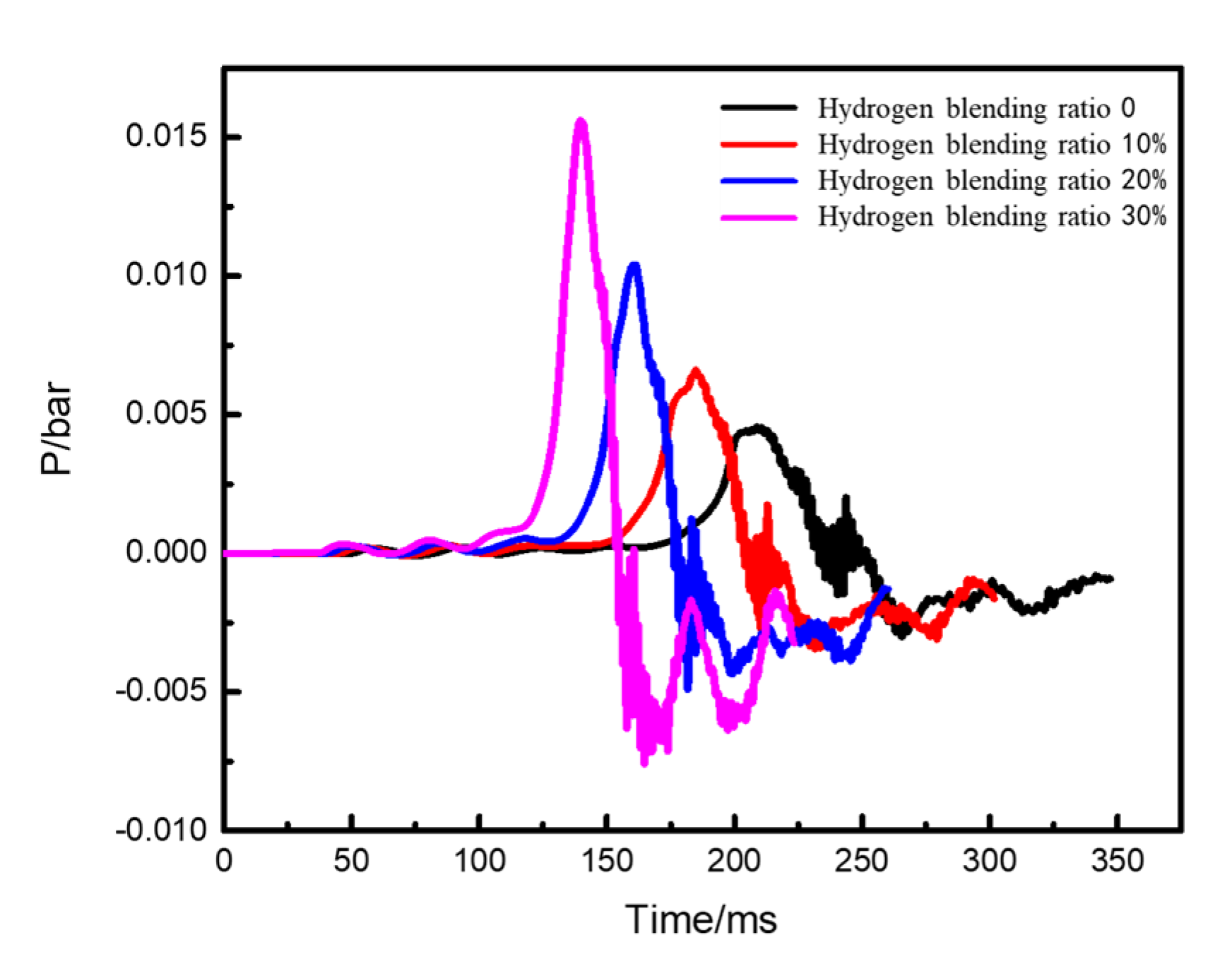
In Figure 22, the static pressure at detection point 4 outside the door exhibits a similar trend in changes under different blending ratios, albeit with varying static pressure and time values. When the hydrogen blending ratio is 0%vol, the peak pressure is 0.0045 bar. As the ratio gradually increases, the explosion peak pressure also rises. With a blending ratio of 30%vol, the explosion pressure reaches 0.015 bar, indicating a 233% increase. Moreover, as the ratio increases, the time to reach the pressure peak significantly advances, and the duration of the pressure peak gradually shortens. In summary, a higher volume concentration of hydrogen blended with natural gas results in an earlier ignition time for the mixed gas explosion and a stronger explosion intensity. By comparing the impact of the explosion on the door under two different working conditions, it is evident that the shock wave generated by the explosion, when the hydrogen blending ratio is less than 30%vol, does not cause significant damage to the door. However, when the door is opened, the shock wave becomes more intense. It is important to note that typical confined spaces in urban gas pipeline networks have structures like windows, doors, and well covers that are easily shattered by shock waves. Therefore, when simulating the explosion of a combustible gas cloud in such confined spaces, it is necessary to incorporate pressure relief plates with varying pressure levels. When the explosion shock wave reaches a certain pressure, the pressure relief plate starts to release pressure, resulting in more severe damage to the outdoor environment due to overpressure.
Spaces that use gas, such as urban residential areas and enclosed gas engineering spaces, should prioritize the maintenance and stability of structures such as windows, doors, and well covers to prevent their destruction by explosion shock waves. Additionally, it is recommended to maintain proper ventilation to avoid the accumulation of gas after a leakage, thereby reducing the risk of explosion.
4. Conclusions
The feasibility of using numerical simulation methods to study the dispersion of gas leaks in confined spaces has been thoroughly verified by conducting leak dispersion simulations with nitrogen and helium instead of natural gas and hydrogen. This research aimed to demonstrate the accuracy of the simulations, and the following conclusions were drawn from the experiment:
- As the leakage flow rate increases, the concentration of oxygen at each detection point decreases more rapidly, and the average concentration of the leaking gas in the kitchen increases.
- The blending of helium accelerates the dispersion of nitrogen. As the proportion of helium increases, the average concentration of the leaking gas in the confined space also increases. On the other hand, if the leaking gas is a blend of hydrogen and natural gas, an increase in the proportion of hydrogen blending leads to an expansion of the combustible range in the kitchen and an increase in risk.
- The leaking gas exhibits a stratification phenomenon in the kitchen, with the concentration gradually decreasing from top to bottom. This stratification is more apparent for small leaks and becomes less pronounced as the leak volume increases.
After comparing multiple sets of experimental data with simulation results, we can draw the following conclusions:
- The trend of the oxygen concentration change at the experimental detection point aligns with the trend observed at the same monitoring point through numerical simulation. Both show a gradual decrease as the leakage time increases. Multiple sets of data were compared and analyzed, revealing that the error range between the experimental data and simulation results of the oxygen concentration at nine monitoring points did not exceed 5% under different leakage flow rates and gas leaks. This falls within an acceptable range. Consequently, it can be concluded that the experimental results are essentially consistent with the simulation results. This fully confirms the feasibility of using the numerical simulation method to study gas diffusion in confined spaces and verifies the accuracy of the simulation.
- The comparison diagram illustrates the streamline of the Y = 1.15m plane for pure nitrogen leakage at various flow rates in the numerical simulation. It shows that as the leakage rate increases, the airflow velocity in the upper part of the kitchen also increases. Consequently, there is an increase in the entrainment of air by the leaking gas and the intensity of the indoor airflow. This provides evidence for the weakening of the gas stratification in the kitchen as the leakage rate increases.
The dispersion of hydrogen-blended natural gas leaks in a domestic kitchen was simulated using Fluent, and the following conclusions were drawn:
- A leak of hydrogen-blended natural gas initially spreads upwards, creating an explosive area larger than the lower explosive limit range at the leak outlet and the top of the kitchen. As the leak continues, the explosive area gradually moves downwards until the kitchen is filled with the hydrogen-blended gas.
- In the case of different proportions of hydrogen blending, a higher proportion of hydrogen leads to a larger volume of the explosive area in the kitchen and a shorter time to fill the kitchen with an explosive volume. Blending hydrogen into the gas promotes the spread of gas after the leak, increasing the risk of leakage.
The explosion of hydrogen-blended natural gas in a domestic kitchen was simulated using FLACS software, and the following conclusions were drawn:
- Under the condition of kitchen doors and windows being closed, the windows start to relieve pressure at 0.1 bar, while the doors relieve pressure at 0.05 bar. The blast wave’s impact range on the window side remains relatively constant and is not affected by changes in the hydrogen blending ratio. However, the shock wave strength increases with an increase in the ratio. When the hydrogen blending ratio reaches 30% by volume, the pressure of the door will be relieved.
- Under the condition of the kitchen doors and windows being open, the overpressure in the space caused by the explosion gradually increases with an increase in the hydrogen blending ratio. The influence range surrounding the kitchen is circular in the horizontal plane, and both the impact range and strength of the shock wave increase with the ratio.
- With an increase in the hydrogen blending ratio, the peak pressure of the explosion significantly increases, the explosion occurs earlier, and the duration of the explosion peak shortens. This indicates that a higher volume concentration of hydrogen blended in natural gas leads to an earlier ignition time and a stronger explosion intensity. To some extent, blending hydrogen increases the hazard of natural gas explosion in confined spaces.
Author Contributions
Conceptualization, H.X., Q.D. and X.H.; methodology, H.X., Q.D. and X.H.; software, D.L.; validation, Q.D. and F.P.; formal analysis, F.P.; investigation, Q.D. and D.L.; resources, H.X., X.H. and F.P.; data curation, Q.D. and D.L.; writing—original draft preparation, H.X. and Q.D.; writing—review and editing, D.L., X.H. and F.P.; visualization, D.L. and Q.D.; supervision, X.H.; project administration, F.P.; funding acquisition, H.X. and X.H. All authors have read and agreed to the published version of the manuscript.
Funding
This study was supported by the National Key Research and Development Program of China, grant number 2022YFB4004400.
Data Availability Statement
The data presented in this study are available on request.
Conflicts of Interest
Author Du Li was employed by the company WISDRI City Environment Protection Engineering Co., Ltd. Author Fengwen Pan was employed by National Center of Technology Innovation for Fuel Cell. The remaining authors declare that the research was conducted in the absence of any commercial or financial relationships that could be construed as a potential conflict of interest.
References
- Prasad, K.; Pitts, W.M.; Yang, J.C. A Numerical Study of the Release and Dispersion of a Buoyant Gas in Partially Confined Spaces. Int. J. Hydrogen Energy 2011, 36, 5200–5210. [Google Scholar] [CrossRef]
- Bernard-Michel, G.; Houssin-Agbomson, D. Comparison of Helium and Hydrogen Releases in 1 M3 and 2 M3 Two Vents Enclosures: Concentration Measurements at Different Flow Rates and for Two Diameters of Injection Nozzle. Int. J. Hydrogen Energy 2017, 42, 7542–7550. [Google Scholar] [CrossRef]
- Afghan Haji Abbas, M.; Kheradmand, S.; Sadoughipour, H. Numerical Study of the Effect of Hydrogen Leakage Position and Direction on Hydrogen Distribution in a Closed Enclosure. Int. J. Hydrogen Energy 2020, 45, 23872–23881. [Google Scholar] [CrossRef]
- Bauwens, C.R.; Dorofeev, S.B. CFD Modeling and Consequence Analysis of an Accidental Hydrogen Release in a Large Scale Facility. Int. J. Hydrogen Energy 2014, 39, 20447–20454. [Google Scholar] [CrossRef]
- Hajji, Y.; Bouteraa, M.; Cafsi, A.E.; Belghith, A.; Bournot, P.; Kallel, F. Dispersion and Behavior of Hydrogen during a Leak in a Prismatic Cavity. Int. J. Hydrogen Energy 2014, 39, 6111–6119. [Google Scholar] [CrossRef]
- Choi, J.; Hur, N.; Kang, S.; Lee, E.D.; Lee, K.-B. A CFD Simulation of Hydrogen Dispersion for the Hydrogen Leakage from a Fuel Cell Vehicle in an Underground Parking Garage. Int. J. Hydrogen Energy 2013, 38, 8084–8091. [Google Scholar] [CrossRef]
- Lowesmith, B.J.; Hankinson, G.; Spataru, C.; Stobbart, M. Gas Build-up in a Domestic Property Following Releases of Methane/Hydrogen Mixtures. Int. J. Hydrogen Energy 2009, 34, 5932–5939. [Google Scholar] [CrossRef]
- Marangon, A.; Carcassi, M.N. Hydrogen–Methane Mixtures: Dispersion and Stratification Studies. Int. J. Hydrogen Energy 2014, 39, 6160–6168. [Google Scholar] [CrossRef]
- Liu, A.; Huang, J.; Li, Z.; Chen, J.; Huang, X.; Chen, K.; Xu, W.B. Numerical Simulation and Experiment on the Law of Urban Natural Gas Leakage and Diffusion for Different Building Layouts. J. Nat. Gas Sci. Eng. 2018, 54, 1–10. [Google Scholar] [CrossRef]
- Middha, P.; Engel, D.; Hansen, O.R. Can the Addition of Hydrogen to Natural Gas Reduce the Explosion Risk? Int. J. Hydrogen Energy 2011, 36, 2628–2636. [Google Scholar] [CrossRef]
- Song, B.; Jiao, W.; Cen, K.; Tian, X.; Zhang, H.; Lu, W. Quantitative Risk Assessment of Gas Leakage and Explosion Accident Consequences inside Residential Buildings. Eng. Fail. Anal. 2021, 122, 105257. [Google Scholar] [CrossRef]
- Zhang, S.; Ma, H.; Huang, X.; Peng, S. Numerical Simulation on Methane-Hydrogen Explosion in Gas Compartment in Utility Tunnel. Process Saf. Environ. Prot. 2020, 140, 100–110. [Google Scholar] [CrossRef]
- Wang, D.; Qian, X.; Yuan, M.; Ji, T.; Xu, W.; Liu, S. Numerical Simulation Analysis of Explosion Process and Destructive Effect by Gas Explosion Accident in Buildings. J. Loss Prev. Process Ind. 2017, 49, 215–227. [Google Scholar] [CrossRef]
- Lowesmith, B.J.; Hankinson, G.; Johnson, D.M. Vapour Cloud Explosions in a Long Congested Region Involving Methane/Hydrogen Mixtures. Process Saf. Environ. Prot. 2011, 89, 234–247. [Google Scholar] [CrossRef]
Figure 1.
Sketch of accidental release on pipeline. Point 1—origin of the pipeline; point 2—leakage inlet point.
Figure 1.
Sketch of accidental release on pipeline. Point 1—origin of the pipeline; point 2—leakage inlet point.

Figure 2.
Geometric drawings of the domestic kitchen.
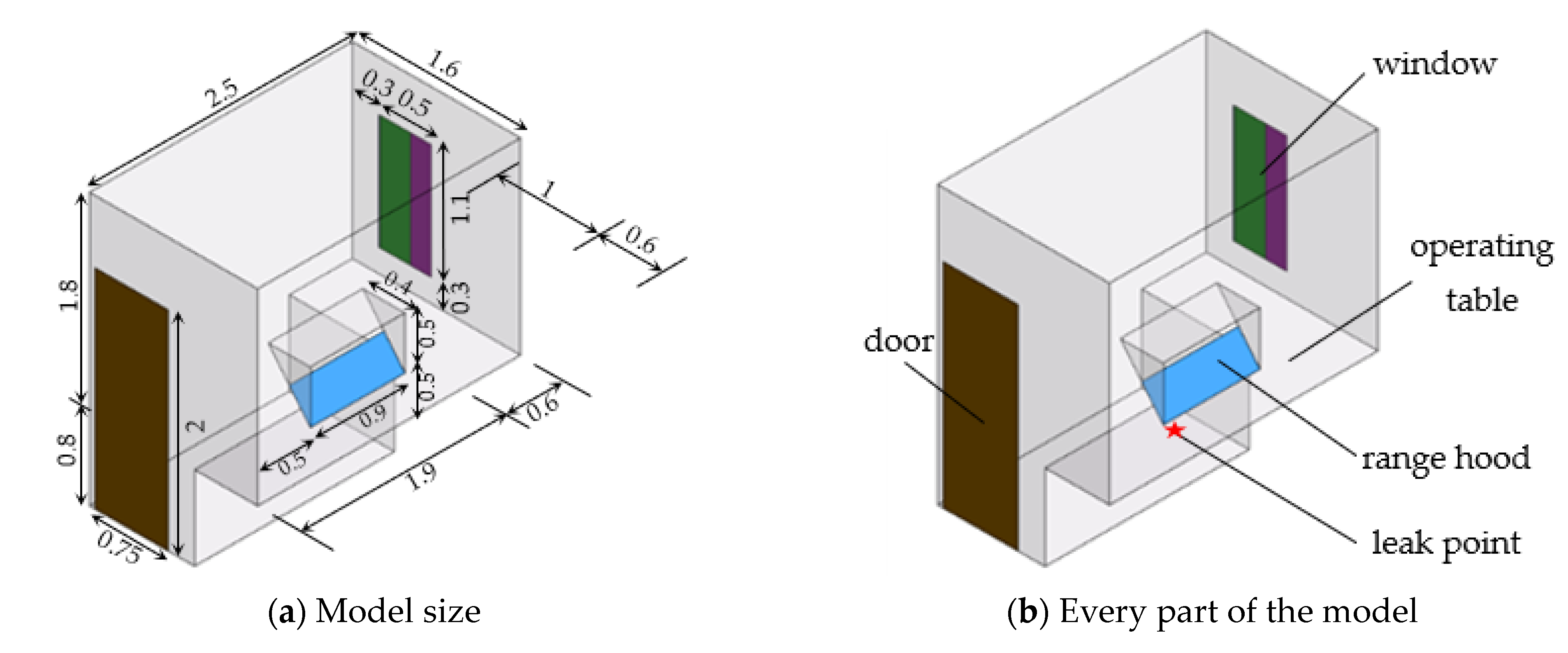
Figure 3.
Location map of oxygen concentration monitoring points.

Figure 4.
A simulation model of an explosion in the kitchen.
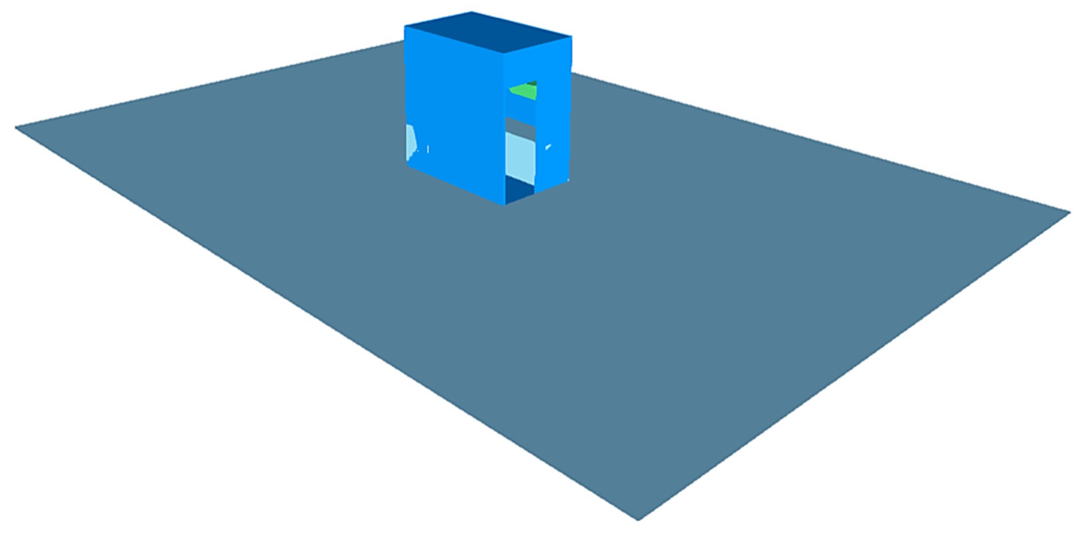
Figure 5.
Detector profile.
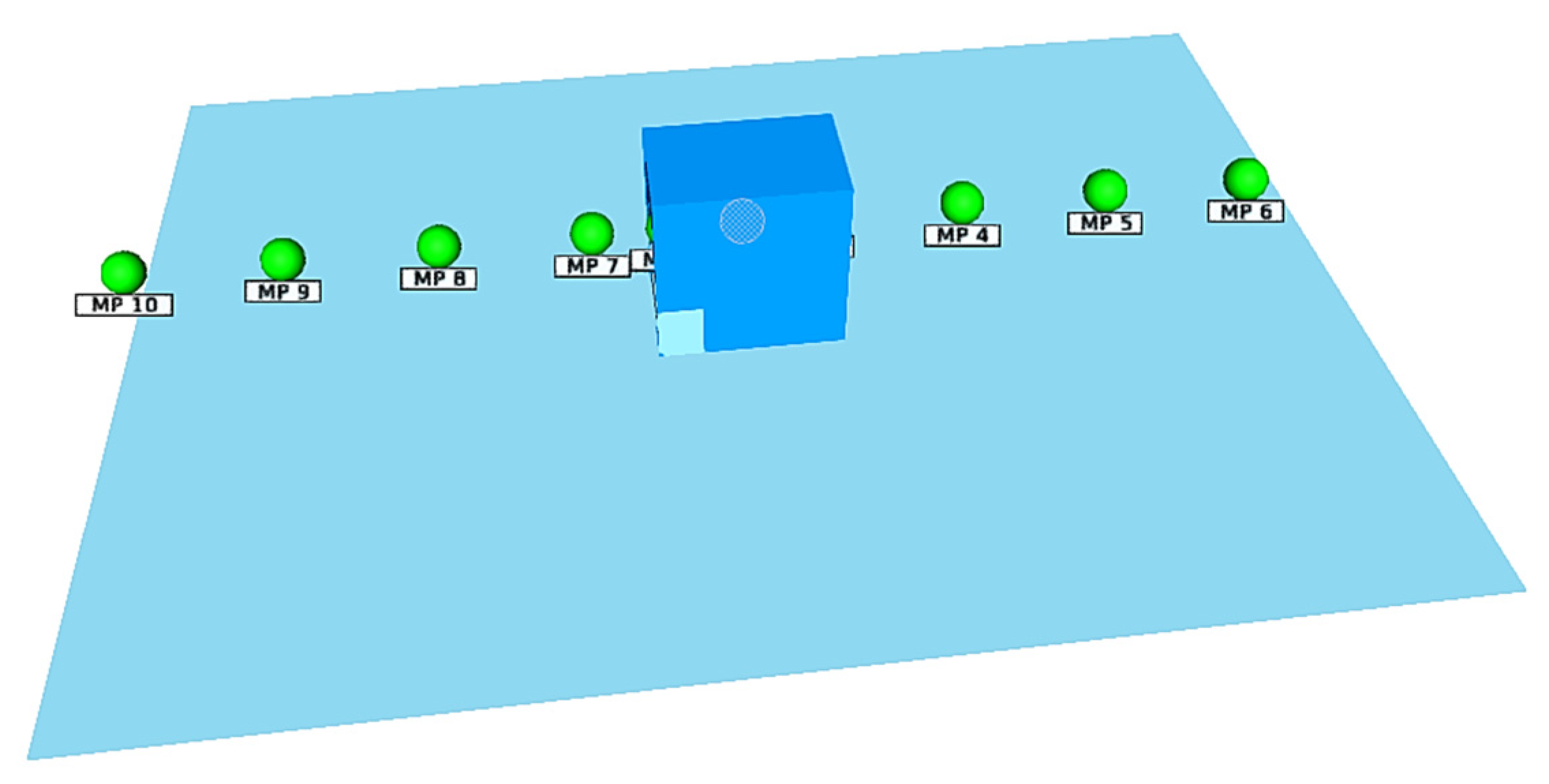
Figure 6.
Mesh division of domestic kitchen model.
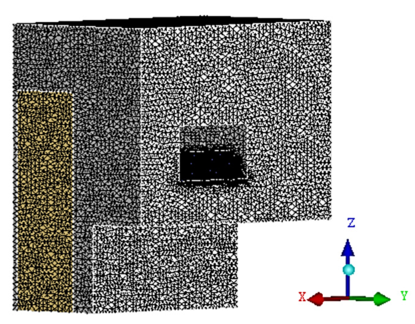
Figure 7.
Kitchen layout.

Figure 8.
Detector layout in the kitchen.

Figure 9.
Variation in oxygen concentration at different heights for different gases at a leakage flow rate of 8 Nm3/h.
Figure 9.
Variation in oxygen concentration at different heights for different gases at a leakage flow rate of 8 Nm3/h.

Figure 10.
Variation in leak gas concentration at a pure nitrogen leak flow rate of 8 Nm3/h.
Figure 11.
Variation in oxygen concentration at different height detection points for pure nitrogen leaks.
Figure 11.
Variation in oxygen concentration at different height detection points for pure nitrogen leaks.
Figure 12.
Y = 1.15 m planar flow distribution at different leakage volumes.
Figure 13.
Comparison of oxygen concentrations at monitoring points 8, 5, 1.
Figure 14.
Distribution of hydrogen blending gas concentrations at 600 s with different ratios (the red shaded areas in the graph are areas where the gas concentration is greater than the lower explosion limit).
Figure 14.
Distribution of hydrogen blending gas concentrations at 600 s with different ratios (the red shaded areas in the graph are areas where the gas concentration is greater than the lower explosion limit).
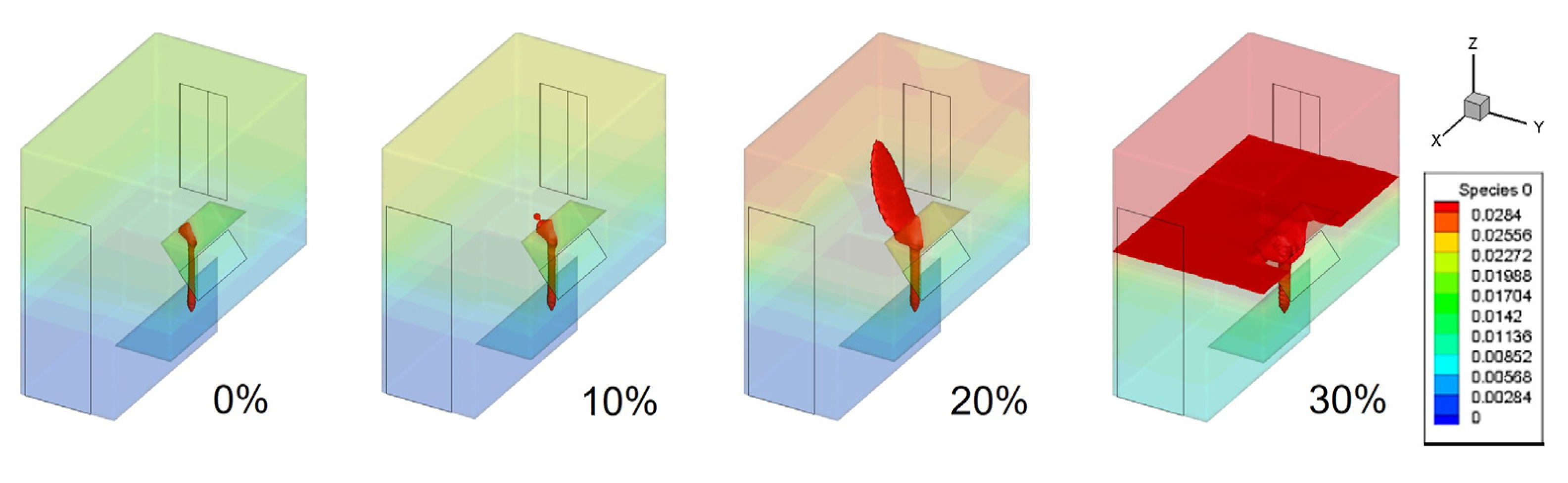
Figure 15.
Distribution of hydrogen blending gas concentrations at 1800 s with different ratios (the red shaded areas in the graph are areas where the gas concentration is greater than the lower explosion limit).
Figure 15.
Distribution of hydrogen blending gas concentrations at 1800 s with different ratios (the red shaded areas in the graph are areas where the gas concentration is greater than the lower explosion limit).

Figure 16.
Graph of combustible gas volume change for different hydrogen blending ratios.
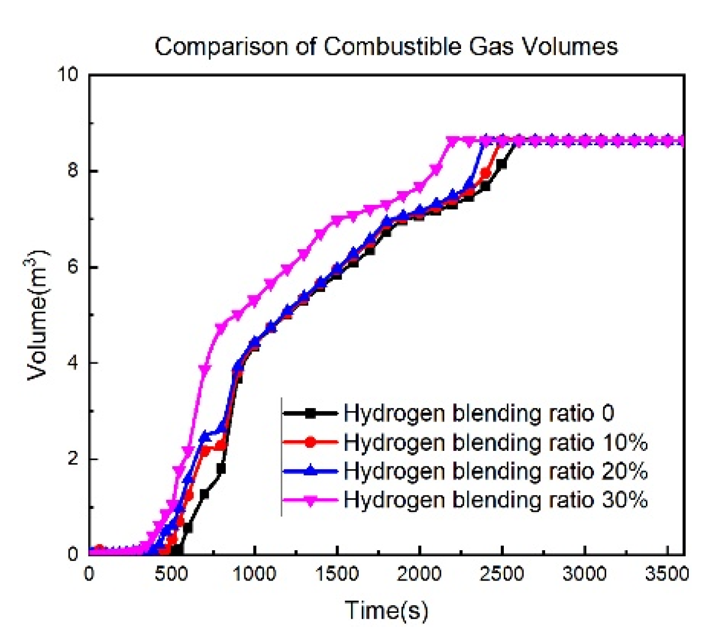
Figure 17.
Dynamic overpressure distribution of kitchen explosion under different ratios of hydrogen when doors and windows are closed.
Figure 17.
Dynamic overpressure distribution of kitchen explosion under different ratios of hydrogen when doors and windows are closed.
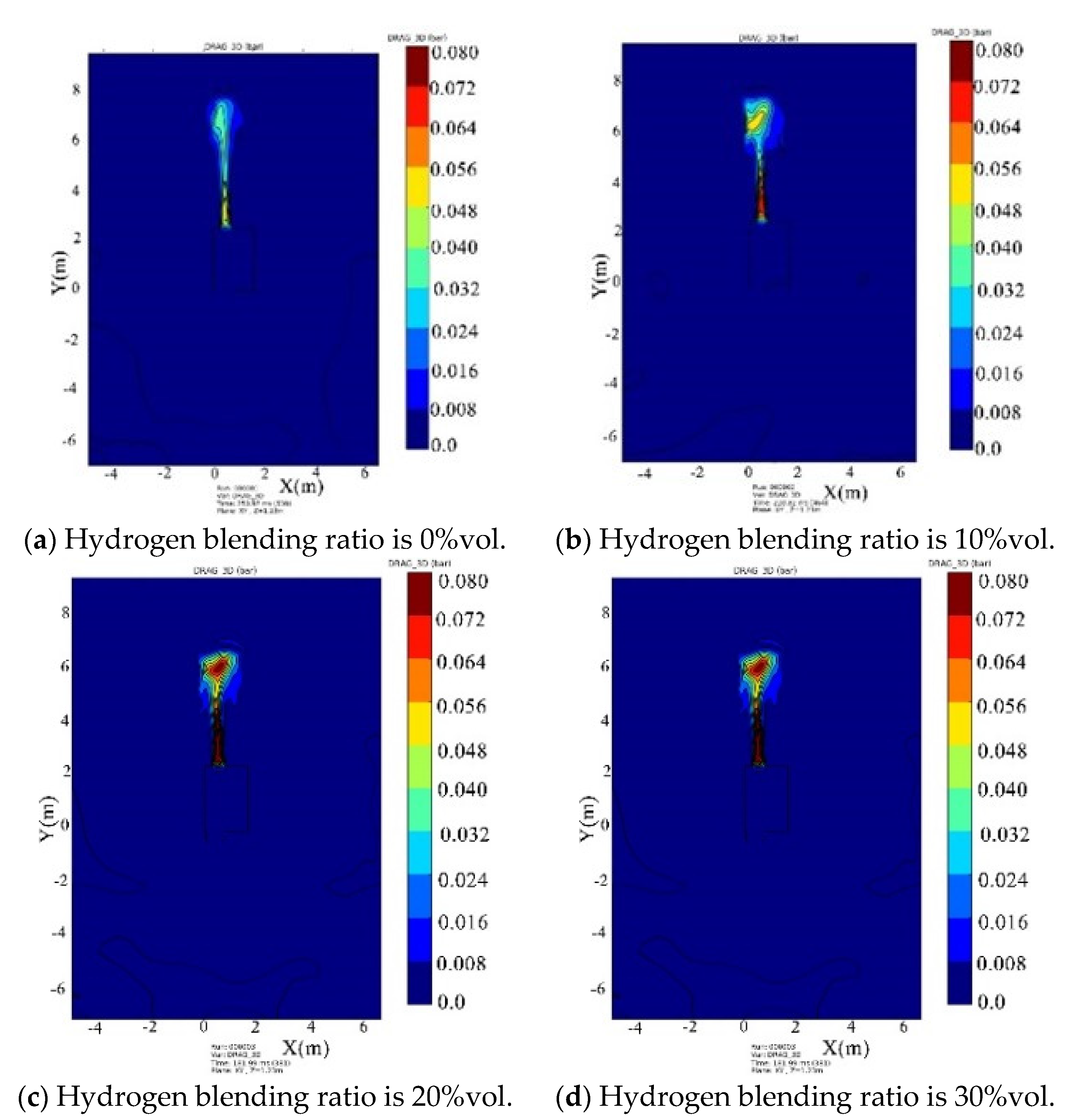
Figure 18.
Diagram of dynamic pressure changes at point 9 (window side) under different ratios of hydrogen.
Figure 18.
Diagram of dynamic pressure changes at point 9 (window side) under different ratios of hydrogen.

Figure 19.
Diagram of dynamic pressure changes at point 4 (door side) under different ratios of hydrogen.
Figure 19.
Diagram of dynamic pressure changes at point 4 (door side) under different ratios of hydrogen.
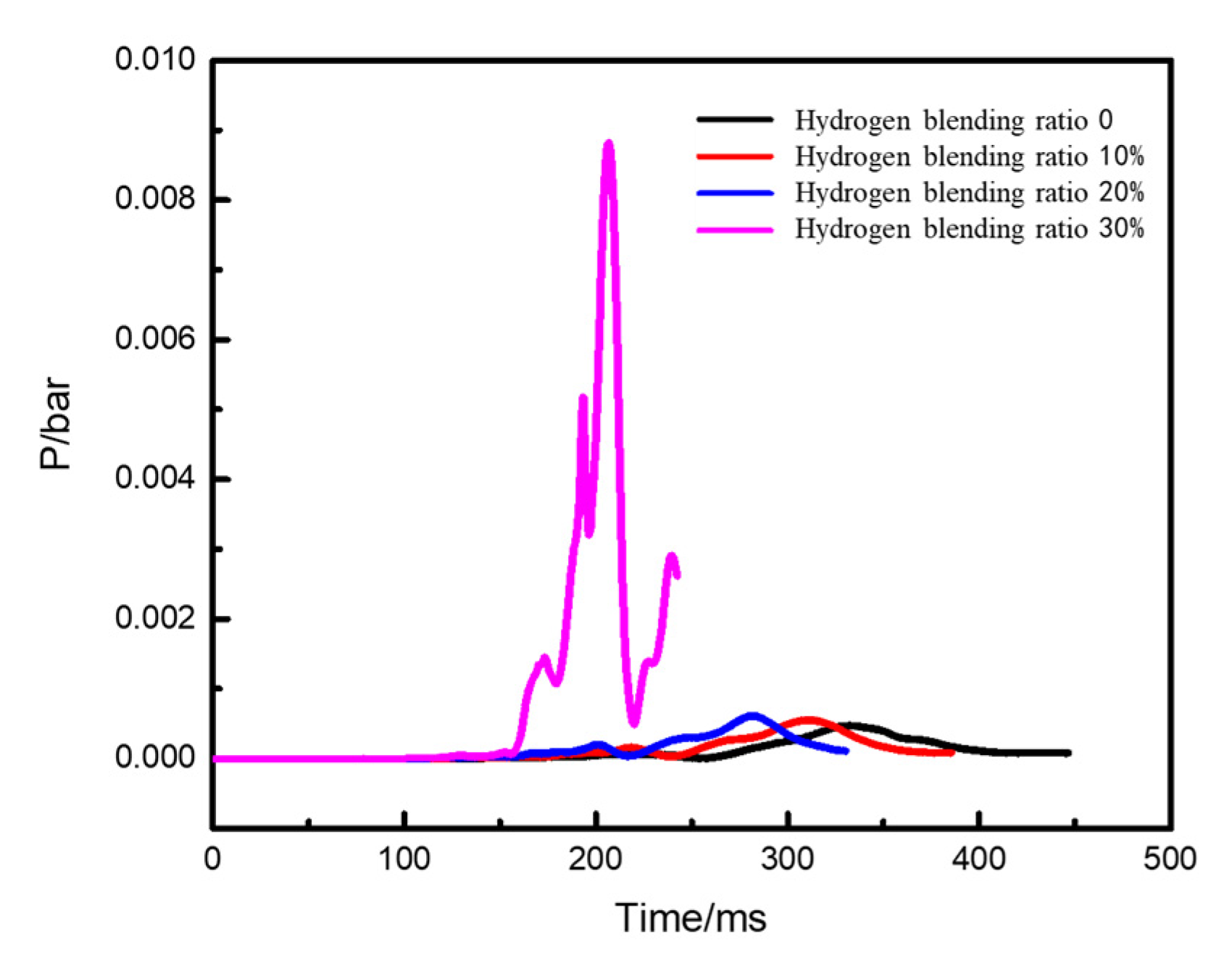
Figure 20.
Dynamic overpressure distribution of kitchen explosion under different ratios of hydrogen when doors and windows are open.
Figure 20.
Dynamic overpressure distribution of kitchen explosion under different ratios of hydrogen when doors and windows are open.

Figure 21.
Diagram of static pressure changes at point 9 (window side) under different ratios of hydrogen.
Figure 21.
Diagram of static pressure changes at point 9 (window side) under different ratios of hydrogen.
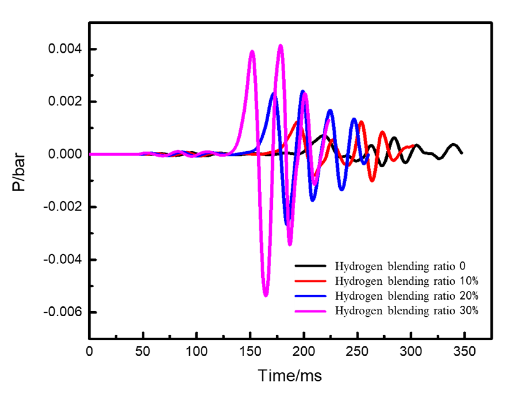
Figure 22.
Diagram of static pressure changes at point 4 (door side) under different ratios of hydrogen.
Figure 22.
Diagram of static pressure changes at point 4 (door side) under different ratios of hydrogen.

Table 1.
Boundary conditions.
| Part | Boundary Condition |
|---|---|
| Operating table | Wall |
| Wall | Wall |
| Doors and windows | Wall |
| Cooker hood | Wall |
| Leak point | Velocity—inlet |
| A gap in the window | Pressure—outlet |
Table 2.
Leakage flow rate and leakage rate of different hydrogen blending ratios.
| Hydrogen Blending Ratios | Leakage Flow Rate (m3/h) | Leakage Rate (m/s) |
|---|---|---|
| 0%vol | 1.85 | 3.067 |
| 10%vol | 1.94 | 3.211 |
| 20%vol | 2.04 | 3.377 |
| 30%vol | 2.30 | 3.570 |
Table 3.
Gas properties.
| Gas Composition | Molar Mass (g/mol) | Density 1 (kg/m3) | Higher Heating Value (kJ/m3) | Lower Explosive Limit (%vol) |
|---|---|---|---|---|
| 100%volHe | 4 | 0.0032 | Null | Null |
| 100%volN2 | 28 | 0.0226 | Null | Null |
| 80%volHe + 20%volN2 | 8.8 | 0.0071 | Null | Null |
| 100%volCH4 | 16 | 0.0129 | 37,768 | 4.60 |
| 90%volCH4 + 10%volH2 | 14.6 | 0.0118 | 35,200 | 4.53 |
| 80%volCH4 + 20%volH2 | 13.2 | 0.0107 | 32,632 | 4.47 |
| 70%volCH4 + 30%volH2 | 11.8 | 0.0095 | 30,064 | 4.40 |
1 P = 2000 Pa, T = 298 K.
Table 4.
Cylinder parameters for experiment.
| Composition of Gas Cylinders | Pressure/MPa | Capacity/L |
|---|---|---|
| N2 | 14.0 ± 0.5 | 40 |
| He | 14.0 ± 0.5 | 40 |
| 80%N2 + 20%He | 9.5 ± 0.5 | 40 |
Disclaimer/Publisher’s Note: The statements, opinions and data contained in all publications are solely those of the individual author(s) and contributor(s) and not of MDPI and/or the editor(s). MDPI and/or the editor(s) disclaim responsibility for any injury to people or property resulting from any ideas, methods, instructions or products referred to in the content. |
© 2024 by the authors. Licensee MDPI, Basel, Switzerland. This article is an open access article distributed under the terms and conditions of the Creative Commons Attribution (CC BY) license (https://creativecommons.org/licenses/by/4.0/).
Share and Cite
MDPI and ACS Style
Xu, H.; Deng, Q.; Huang, X.; Li, D.; Pan, F. Simulation and Experimental Verification of Dispersion and Explosion of Hydrogen–Methane Mixture in a Domestic Kitchen. Energies 2024, 17, 2320. https://doi.org/10.3390/en17102320
AMA Style
Xu H, Deng Q, Huang X, Li D, Pan F. Simulation and Experimental Verification of Dispersion and Explosion of Hydrogen–Methane Mixture in a Domestic Kitchen. Energies. 2024; 17(10):2320. https://doi.org/10.3390/en17102320
Chicago/Turabian StyleXu, Haidong, Qiang Deng, Xiaomei Huang, Du Li, and Fengwen Pan. 2024. "Simulation and Experimental Verification of Dispersion and Explosion of Hydrogen–Methane Mixture in a Domestic Kitchen" Energies 17, no. 10: 2320. https://doi.org/10.3390/en17102320
Note that from the first issue of 2016, this journal uses article numbers instead of page numbers. See further details here.