
SNR Prediction with ANN for UAV Applications in IoT Networks Based on Measurements

 , and
, and
Abstract
:1. Introduction
- 1.
- Verify the necessity of downlink and uplink analysis due to the reciprocity principle [11].
- 2.
- SNR downlink and uplink measurement campaigns using a UAV to understand how the signal behaves in a suburban and densely forested environment, considering both Line-of-Sight (LOS) and Non-Line-of-Sight (NLOS) situations.
- 3.
- Different SNR regression models and an ANN-based prediction model were established to represent the signal within Amazon cities, which could be reproduced in similar environments. Additionally, the proposed models could assist in improving LoRa ADR technology.
2. Related Works
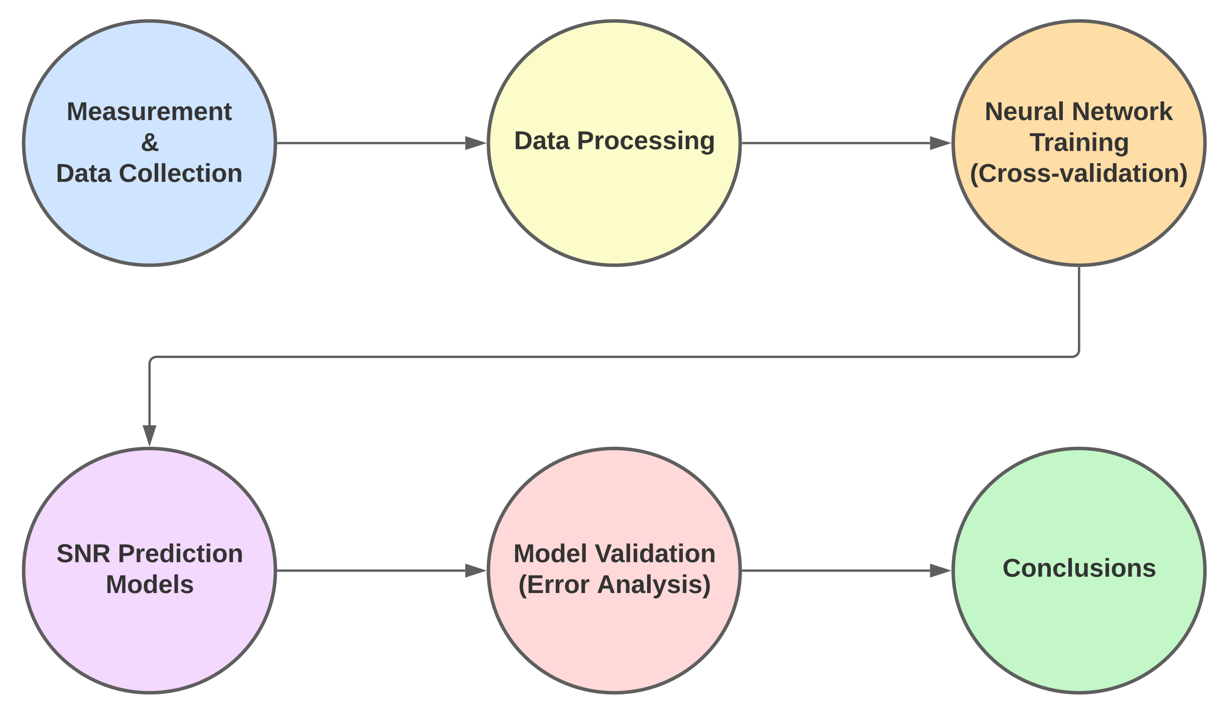
3. Methodology
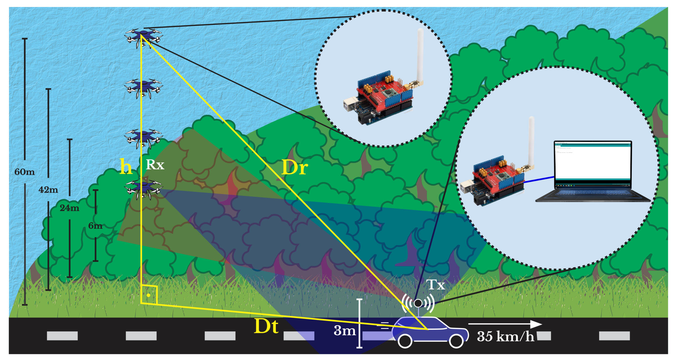
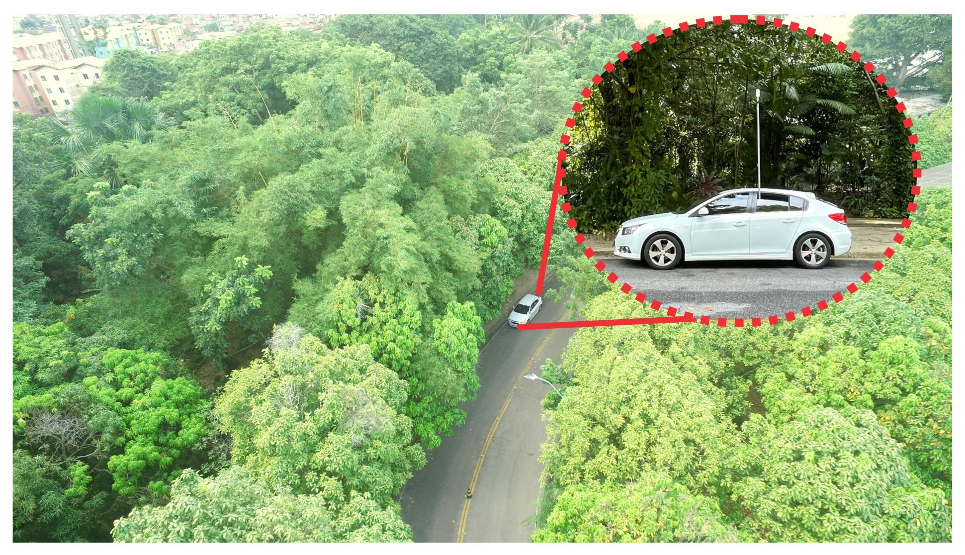
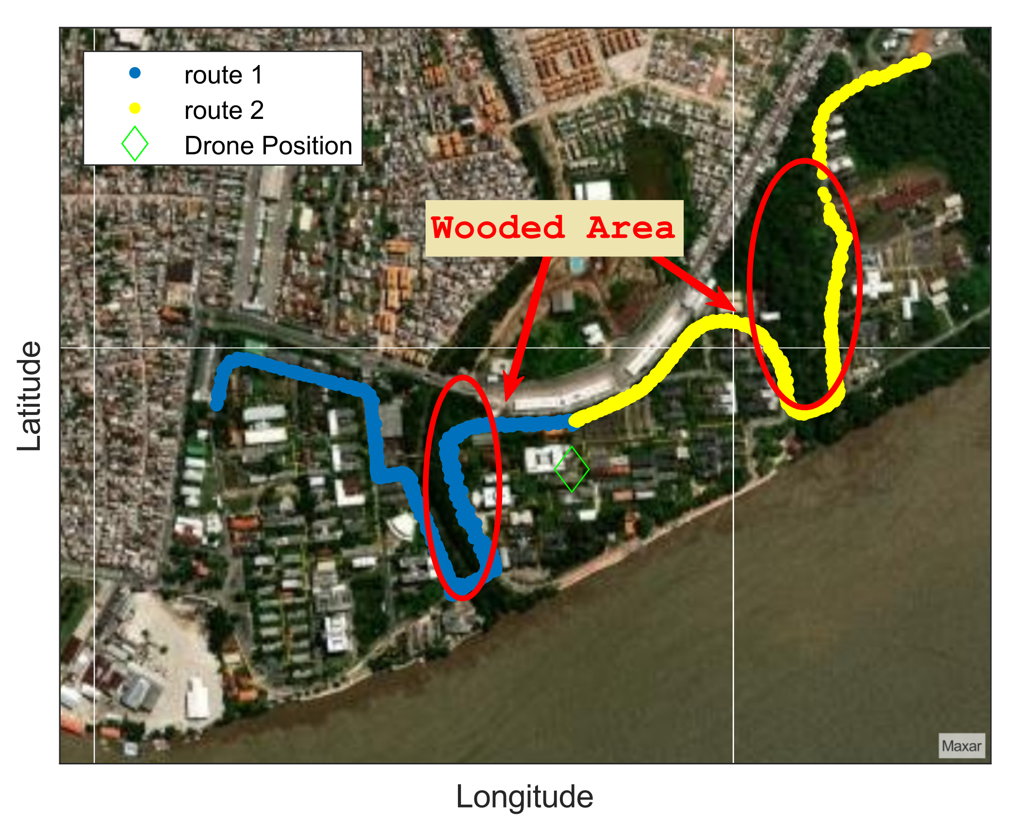
3.1. Measurement Campaign
3.2. Data Preprocessing
3.2.1. Distance between UAV and Vehicle
3.2.2. Path Loss Calculation
3.3. Collected Data
3.4. Artificial Neural Network
3.4.1. Generalized Regression Neural Network
3.4.2. Neural Network Training
4. Results
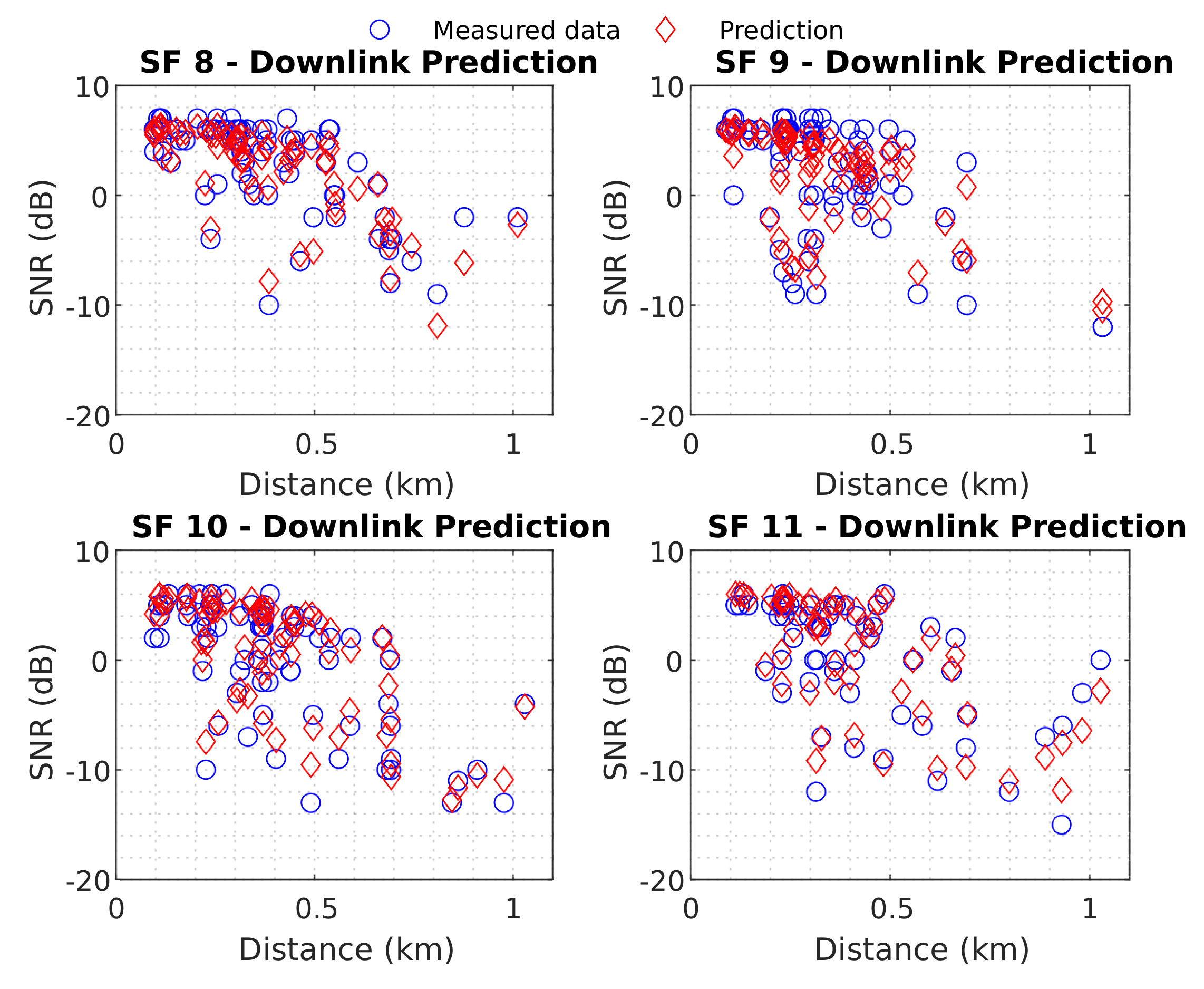
4.1. Downlink
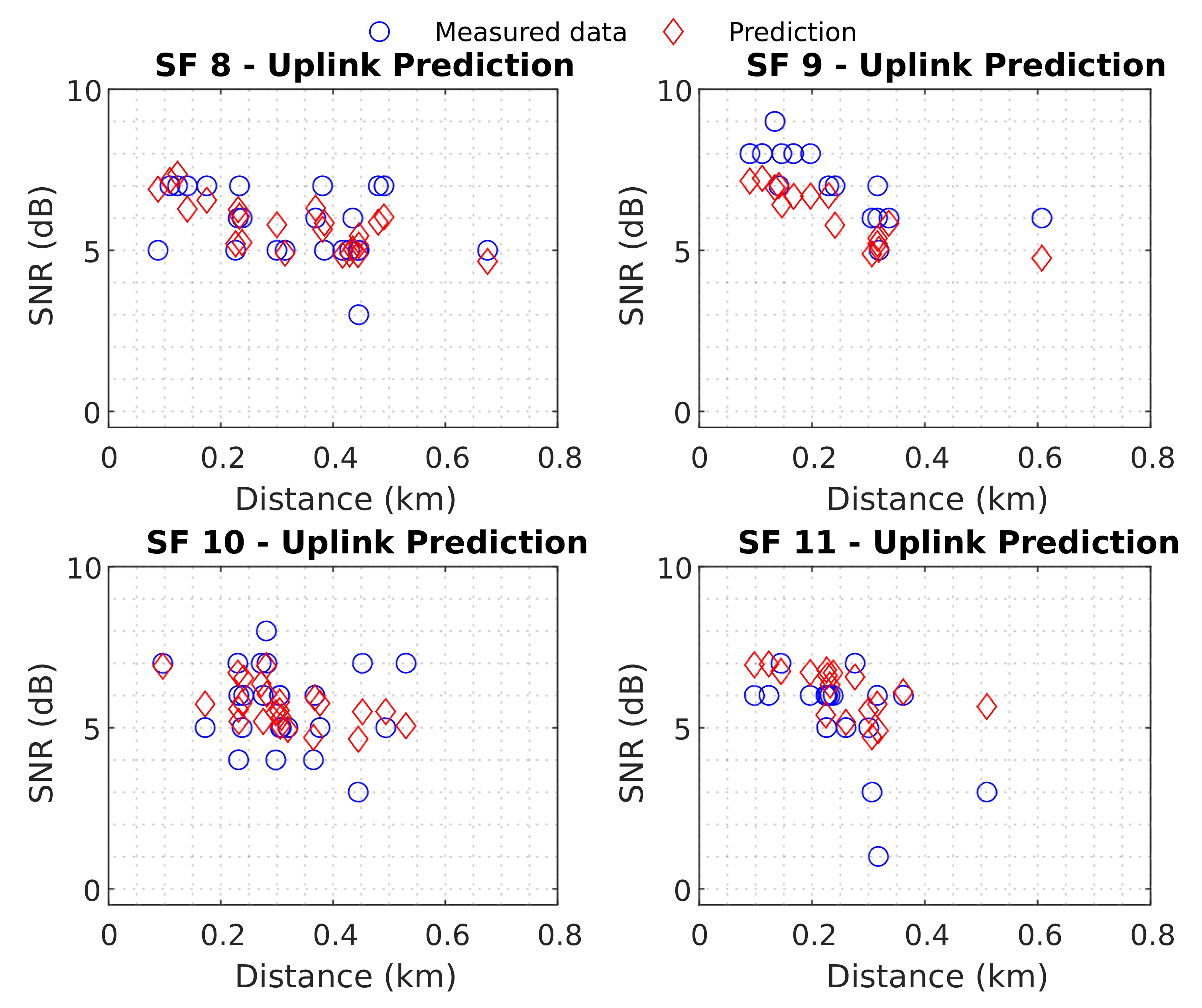
4.2. Uplink
5. Conclusions
Author Contributions
Funding
Institutional Review Board Statement
Informed Consent Statement
Data Availability Statement
Acknowledgments
Conflicts of Interest
Appendix A. Downlink Regressions

| Regression | Height | SF | Coefficients (a,b,c) | RMSE | SF | ||
|---|---|---|---|---|---|---|---|
| Linear | 6 | −28.870 | 7.629 | 4.0472 | 4.0314 | ||
| Power | 6 | 8 | 34.670 | −0.154 | −43.290 | 3.9431 | 3.9121 |
| Sigmoid | 6 | 10.210 | −3.687 | 14.440 | 3.8993 | 3.8688 | |
| Linear | 6 | −31.520 | 7.820 | 4.5076 | 4.4925 | ||
| Power | 6 | 9 | −39.940 | 0.294 | 25.940 | 4.4773 | 4.4471 |
| Sigmoid | 6 | 9.462 | −5.808 | 11.780 | 4.4680 | 4.4379 | |
| Linear | 6 | −26.920 | 6.290 | 4.7338 | 4.7178 | ||
| Power | 6 | 10 | −54.420 | 0.179 | 41.500 | 4.6577 | 4.6261 |
| Sigmoid | 6 | 9.434 | −5.929 | 12.130 | 4.6758 | 4.6441 | |
| Linear | 6 | −25.280 | 5.380 | 4.0767 | 4.0597 | ||
| Power | 6 | 11 | −30.340 | 0.489 | 14.150 | 4.0206 | 3.987 |
| Sigmoid | 6 | 7.263 | −16.150 | 5.301 | 4.1047 | 4.0703 | |
| Linear | 24 | −15.080 | 7.904 | 3.1730 | 3.1647 | ||
| Power | 24 | 8 | −14.800 | 1.151 | 7.140 | 3.1779 | 3.1612 |
| Sigmoid | 24 | 8.608 | −10.870 | 3.669 | 3.1681 | 3.1515 | |
| Linear | 24 | −22.900 | 10.000 | 2.9064 | 2.8983 | ||
| Power | 24 | 9 | −23.000 | 1.230 | 8.505 | 2.8970 | 2.8809 |
| Sigmoid | 24 | 10.300 | −14.980 | 4.450 | 2.8423 | 2.8265 | |
| Linear | 24 | −24.870 | 9.432 | 3.6520 | 3.6413 | ||
| Power | 24 | 10 | −25.640 | 1.381 | 7.089 | 3.6237 | 3.6024 |
| Sigmoid | 24 | 10.050 | −21.470 | 3.912 | 3.5858 | 3.5648 | |
| Linear | 24 | −18.790 | 7.989 | 3.1916 | 3.1809 | ||
| Power | 24 | 11 | −19.190 | 0.925 | 8.603 | 3.2002 | 3.1788 |
| Sigmoid | 24 | 9.063 | −11.030 | 4.778 | 3.0645 | 3.0440 | |
| Linear | 42 | −13.790 | 8.467 | 2.4249 | 2.4199 | ||
| Power | 42 | 8 | −13.380 | 1.147 | 7.734 | 2.4254 | 2.4154 |
| Sigmoid | 42 | 9.005 | −7.326 | 4.042 | 2.3673 | 2.3575 | |
| Linear | 42 | −17.330 | 9.243 | 3.0311 | 3.0232 | ||
| Power | 42 | 9 | −17.180 | 1.259 | 7.932 | 3.0260 | 3.0102 |
| Sigmoid | 42 | 9.620 | −10.960 | 4.029 | 3.0098 | 2.9941 | |
| Linear | 42 | −17.670 | 9.082 | 2.7153 | 2.7085 | ||
| Power | 42 | 10 | −16.820 | 1.335 | 7.261 | 2.6911 | 2.6775 |
| Sigmoid | 42 | 9.528 | −13.610 | 3.631 | 2.6569 | 2.6435 | |
| Linear | 42 | −13.880 | 7.422 | 2.5616 | 2.5537 | ||
| Power | 42 | 11 | −13.570 | 1.107 | 6.880 | 2.5670 | 2.5511 |
| Sigmoid | 42 | 8.270 | −8.635 | 3.925 | 2.5074 | 2.4918 | |
| Linear | 60 | −12.530 | 9.218 | 2.4909 | 2.4852 | ||
| Power | 60 | 8 | −12.950 | 1.803 | 7.128 | 2.4199 | 2.4088 |
| Sigmoid | 60 | 9.971 | −11.790 | 3.012 | 2.4206 | 2.4094 | |
| Linear | 60 | −17.890 | 10.530 | 2.2726 | 2.2671 | ||
| Power | 60 | 9 | −17.510 | 1.841 | 7.320 | 2.0562 | 2.0462 |
| Sigmoid | 60 | 11.300 | −22.900 | 2.844 | 2.0686 | 2.0586 | |
| Linear | 60 | −17.850 | 9.730 | 2.6396 | 2.6328 | ||
| Power | 60 | 10 | −16.510 | 1.438 | 7.379 | 2.5955 | 2.5819 |
| Sigmoid | 60 | 9.972 | −14.440 | 3.466 | 2.5609 | 2.5475 | |
| Linear | 60 | −16.400 | 8.690 | 2.8043 | 2.7953 | ||
| Power | 60 | 11 | −15.370 | 1.665 | 5.990 | 2.7101 | 2.6928 |
| Sigmoid | 60 | 9.441 | −15.950 | 3.148 | 2.6859 | 2.6687 | |
Appendix B. Uplink Regressions
| Regression | Height | SF | Coefficients (a,b,c) | RMSE | SF | ||
|---|---|---|---|---|---|---|---|
| Linear | 6 | 1.658 | 6.035 | 0.9550 | 0.9349 | ||
| Power | 6 | 8 | 4.347 | 2.025 | 6.168 | 0.9751 | 0.9335 |
| Sigmoid | 6 | 5.935 | 6.920 | 7.630 | 0.9752 | 0.9337 | |
| Linear | 6 | −1.275 | 7.382 | 0.7708 | 0.7539 | ||
| Power | 6 | 9 | 7.096 | −0.027 | −0.303 | 0.7903 | 0.7551 |
| Sigmoid | 6 | 7.682 | 4.769 | 2.859 | 0.7890 | 0.7538 | |
| Linear | 6 | 4.063 | 6.666 | 0.7460 | 0.7222 | ||
| Power | 6 | 10 | 4.121 | 0.285 | 4.917 | 0.7701 | 0.7203 |
| Sigmoid | 6 | 0.322 | 8.087 | 7.291 | 0.7692 | 0.7194 | |
| Linear | 6 | −1.262 | 6.345 | 0.6295 | 0.6081 | ||
| Power | 6 | 11 | −24.850 | 0.012 | 30.420 | 0.6438 | 0.5993 |
| Sigmoid | 6 | 6.593 | 5.889 | 16.930 | 0.6418 | 0.5974 | |
| Linear | 24 | −2.088 | 6.220 | 1.1710 | 1.1605 | ||
| Power | 24 | 8 | −94.920 | 0.007 | 99.610 | 1.1602 | 1.1392 |
| Sigmoid | 24 | 17.180 | −182.500 | 0.186 | 1.1826 | 1.1612 | |
| Linear | 24 | −6.536 | 7.860 | 0.9214 | 0.9106 | ||
| Power | 24 | 9 | 9.627 | −0.122 | −5.307 | 0.9172 | 0.8955 |
| Sigmoid | 24 | 8.249 | 5.273 | 12.330 | 0.9185 | 0.8968 | |
| Linear | 24 | −4.794 | 7.209 | 1.1188 | 1.1057 | ||
| Power | 24 | 10 | 0.014 | −2.129 | 5.426 | 1.0495 | 1.0248 |
| Sigmoid | 24 | 9.350 | 5.546 | 23.570 | 1.0528 | 1.0281 | |
| Linear | 24 | −7.573 | 6.721 | 1.4725 | 1.4545 | ||
| Power | 24 | 11 | −89.050 | 0.022 | 90.950 | 1.4522 | 1.4163 |
| Sigmoid | 24 | −0.689 | 2.625 | 2.549 | 1.4456 | 1.4099 | |
| Linear | 42 | −5.093 | 6.947 | 1.3183 | 1.3104 | ||
| Power | 42 | 8 | 0.405 | −0.904 | 3.964 | 1.2729 | 1.2576 |
| Sigmoid | 42 | 8.441 | 4.788 | 15.410 | 1.2576 | 1.2425 | |
| Linear | 42 | −3.739 | 7.675 | 0.8245 | 0.8171 | ||
| Power | 42 | 9 | 79.880 | −0.009 | −74.310 | 0.8496 | 0.8343 |
| Sigmoid | 42 | 0.083 | 8.063 | −3.317 | 0.8296 | 0.8146 | |
| Linear | 42 | −8.829 | 8.343 | 1.1521 | 1.1411 | ||
| Power | 42 | 10 | 67.430 | −0.030 | −64.460 | 1.1660 | 1.1438 |
| Sigmoid | 42 | 2.136 | 23.650 | −2.993 | 1.1550 | 1.1330 | |
| Linear | 42 | −5.828 | 6.877 | 1.2702 | 1.2560 | ||
| Power | 42 | 11 | 124.900 | −0.011 | −121.600 | 1.3233 | 1.2936 |
| Sigmoid | 42 | 0.029 | 6.358 | −6.235 | 1.2753 | 1.2466 | |
| Linear | 60 | −3.559 | 7.190 | 0.9179 | 0.9130 | ||
| Power | 60 | 8 | 46.250 | −0.023 | −41.530 | 0.9247 | 0.9148 |
| Sigmoid | 60 | 3.316 | 21.100 | −1.642 | 0.9215 | 0.9117 | |
| Linear | 60 | −5.322 | 8.180 | 0.8728 | 0.8664 | ||
| Power | 60 | 9 | 76.784 | −0.018 | −71.984 | 0.8816 | 0.8687 |
| Sigmoid | 60 | 4.069 | 27.424 | −2.471 | 0.8741 | 0.8613 | |
| Linear | 60 | −3.635 | 7.058 | 1.0334 | 1.0244 | ||
| Power | 60 | 10 | −30.258 | 0.038 | 34.800 | 1.0348 | 1.0168 |
| Sigmoid | 60 | 5.131 | 24.155 | −5.361 | 1.0372 | 1.0191 | |
| Linear | 60 | −2.285 | 5.877 | 1.3721 | 1.3594 | ||
| Power | 60 | 11 | −84.487 | 0.010 | 88.584 | 1.3622 | 1.3367 |
| Sigmoid | 60 | 8.323 | 4.908 | 21.020 | 1.3362 | 1.3112 | |
References
- Popovski, P.; Trillingsgaard, K.F.; Simeone, O.; Durisi, G. 5G Wireless Network Slicing for eMBB, URLLC, and mMTC: A Communication-Theoretic View. IEEE Access 2018, 6, 55765–55779. [Google Scholar] [CrossRef]
- Lathi, B.P. Modern Digital and Analog Communications Systems; Oxford University Press Inc.: Oxford, UK, 2009. [Google Scholar]
- SEMTECH. AN1200.22 LoRa™ Modulation Basics, Application Note. 2015. Available online: https://www.frugalprototype.com/wp-content/uploads/2016/08/an1200.22.pdf (accessed on 12 March 2022).
- Marchese, M.; Moheddine, A.; Patrone, F. Towards Increasing the LoRa Network Coverage: A Flying Gateway. In Proceedings of the 2019 International Symposium on Advanced Electrical and Communication Technologies (ISAECT), Rome, Italy, 27–29 November 2019. [Google Scholar] [CrossRef]
- Bocker, S.; Arendt, C.; Jorke, P.; Wietfeld, C. LPWAN in the Context of 5G: Capability of LoRaWAN to Contribute to mMTC. In Proceedings of the 2019 IEEE 5th World Forum on Internet of Things (WF-IoT), Limerick, Ireland, 15–18 April 2019. [Google Scholar] [CrossRef]
- Valavanis, K. Handbook of Unmanned Aerial Vehicles; Springer: Dordrecht, The Netherland, 2014. [Google Scholar]
- Bupe, P.; Haddad, R.; Rios-Gutierrez, F. Relief and emergency communication network based on an autonomous decentralized UAV clustering network. In Proceedings of the SoutheastCon 2015, Fort Lauderdale, FL, USA, 9–12 April 2015; pp. 1–8. [Google Scholar] [CrossRef]
- Erdelj, M.; Natalizio, E.; Chowdhury, K.R.; Akyildiz, I.F. Help from the Sky: Leveraging UAVs for Disaster Management. IEEE Pervasive Comput. 2017, 16, 24–32. [Google Scholar] [CrossRef]
- Wu, L.; He, D.; Ai, B.; Wang, J.; Qi, H.; Guan, K.; Zhong, Z. Artificial Neural Network Based Path Loss Prediction for Wireless Communication Network. IEEE Access 2020, 8, 199523–199538. [Google Scholar] [CrossRef]
- SEMTECH. SX1276/77/78/79-137 MHz to 1020 MHz Low Power Long Range Transceiver, Application Note. 2016. Available online: https://www.mouser.com/datasheet/2/761/sx1276-1278113.pdf (accessed on 15 March 2022).
- Balanis, C.A. Antenna Theory, 4th ed.; John Wiley & Sons: Hoboken, NJ, USA, 2015; Chapter 3. [Google Scholar]
- Mozaffari, M.; Saad, W.; Bennis, M.; Nam, Y.H.; Debbah, M. A Tutorial on UAVs for Wireless Networks: Applications, Challenges, and Open Problems. IEEE Commun. Surv. Tutorials 2019, 21, 2334–2360. [Google Scholar] [CrossRef] [Green Version]
- Ahmad, A.; Cheema, A.A.; Finlay, D. A survey of radio propagation channel modelling for low altitude flying base stations. Comput. Netw. 2020, 171, 107122. [Google Scholar] [CrossRef]
- Moheddine, A.; Patrone, F.; Marchese, M. UAV and IoT Integration: A Flying Gateway. In Proceedings of the 2019 26th IEEE International Conference on Electronics, Circuits and Systems (ICECS), Genoa, Italy, 27–29 November 2019. [Google Scholar] [CrossRef]
- Park, S.; Yun, S.; Kim, H.; Kwon, R.; Ganser, J.; Anthony, S. Forestry Monitoring System using LoRa and Drone. In Proceedings of the Proceedings of the 8th International Conference on Web Intelligence, Mining and Semantics, Novi Sad, Serbia, 25–27 June 2018. [CrossRef]
- Chall, R.E.; Lahoud, S.; Helou, M.E. LoRaWAN Network: Radio Propagation Models and Performance Evaluation in Various Environments in Lebanon. IEEE Internet Things J. 2019, 6, 2366–2378. [Google Scholar] [CrossRef]
- Dambal, V.A.; Mohadikar, S.; Kumbhar, A.; Guvenc, I. Improving LoRa Signal Coverage in Urban and Sub-Urban Environments with UAVs. In Proceedings of the 2019 International Workshop on Antenna Technology (iWAT), Miami, FL, USA, 3–6 March 2019. [Google Scholar] [CrossRef] [Green Version]
- Da Silva, D.K.N.; Eras, L.E.C.; Barrsos, F.J.B.; Cavalcante, G.P.S. VHF–UHF Electric Field Prediction for Amazon City Using Dyadic Green’s Function. Wirel. Pers. Commun. 2020, 113, 2301–2326. [Google Scholar] [CrossRef]
- Nielsen, M. Neural Networks and Deep Learning. 2015. Available online: http://neuralnetworksanddeeplearning.com/chap4.html (accessed on 23 January 2022).
- Braga, A.D.S.; Cruz, H.A.O.D.; Eras, L.E.C.; Araújo, J.P.L.; Neto, M.C.A.; Silva, D.K.N.; Cavalcante, G.P.S. Radio Propagation Models Based on Machine Learning Using Geometric Parameters for a Mixed City-River Path. IEEE Access 2020, 8, 146395–146407. [Google Scholar] [CrossRef]
- Benmus, T.A.; Abboud, R.; Shatter, M.K. Neural network approach to model the propagation path loss for great Tripoli area at 900, 1800, and 2100 MHz bands. In Proceedings of the 2015 16th International Conference on Sciences and Techniques of Automatic Control and Computer Engineering (STA), Monastir, Tunisia, 21–23 December 2015; pp. 793–798. [Google Scholar] [CrossRef]
- Ayadi, M.; Ben Zineb, A.; Tabbane, S. A UHF Path Loss Model Using Learning Machine for Heterogeneous Networks. IEEE Trans. Antennas Propag. 2017, 65, 3675–3683. [Google Scholar] [CrossRef]
- Mod Rofi, A.S.; Habaebi, M.H.; Islam, M.R.; Basahel, A. LoRa Channel Propagation Modelling using Artificial Neural Network. In Proceedings of the 2021 8th International Conference on Computer and Communication Engineering (ICCCE), Kuala Lumpur, Malaysia, 22–23 June 2021; pp. 58–62. [Google Scholar] [CrossRef]
- Wasserman, P. Advanced Methods in Neural Computing; Van Nostrand Reinhold: New York, NY, USA, 1993. [Google Scholar]
- Al-Mahasneh, A.J.; Anavatti, S.; Garratt, M.; Pratama, M. Applications of General Regression Neural Networks in Dynamic Systems. In Digital Systems; Asadpour, V., Ed.; IntechOpen: Rijeka, Croatia, 2018; Chapter 8. [Google Scholar] [CrossRef] [Green Version]
- Witten, I.; Frank, E.; Hall, M.A.; Pal, C.J. Data Mining; Elsevier: Oxford, UK, 2017; Chapter 5. [Google Scholar]
- Gholamiangonabadi, D.; Kiselov, N.; Grolinger, K. Deep Neural Networks for Human Activity Recognition With Wearable Sensors: Leave-One-Subject-Out Cross-Validation for Model Selection. IEEE Access 2020, 8, 133982–133994. [Google Scholar] [CrossRef]


| SF | Regression | Coefficients | RMSE | SD | ||
|---|---|---|---|---|---|---|
| Linear | a = −13.7900 | b = 8.4670 | 2.4249 | 2.4199 | ||
| 8 | Power | a = −13.3800 | b = 1.1470 | c = 7.7340 | 2.4254 | 2.4154 |
| Sigmoid | a = 9.0050 | b = −7.3260 | c = 4.0420 | 2.3673 | 2.3575 | |
| Linear | a = −17.3300 | b = 9.2430 | 3.0311 | 3.0232 | ||
| 9 | Power | a = −17.1800 | b = 1.2590 | c = 7.9320 | 3.0260 | 3.0102 |
| Sigmoid | a = 9.6200 | b = −10.9600 | c = 4.0290 | 3.0098 | 2.9941 | |
| Linear | a = −17.6700 | b = 9.0820 | 2.7153 | 2.7085 | ||
| 10 | Power | a = −16.8200 | b = 1.3350 | c = 7.2610 | 2.6911 | 2.6775 |
| Sigmoid | a = 9.5280 | b = −13.6100 | c = 3.6310 | 2.6569 | 2.6435 | |
| Linear | a = −13.8803 | b = 7.4222 | 2.5616 | 2.5537 | ||
| 11 | Power | a = −13.5700 | b = 1.1070 | c = 6.8800 | 2.5670 | 2.5511 |
| Sigmoid | a = 8.2700 | b = −8.6359 | c = 3.9258 | 2.5074 | 2.4918 | |
| SF | RMSE | SD |
|---|---|---|
| 8 | 1.2322 | 1.2010 |
| 9 | 1.6623 | 1.6730 |
| 10 | 1.3511 | 1.2600 |
| 11 | 1.3183 | 1.2819 |
| SF | Regression | Coefficients | RMSE | SD | ||
|---|---|---|---|---|---|---|
| Linear | a = −5.0930 | b = 6.9470 | 1.3183 | 1.3104 | ||
| 8 | Power | a = 0.4058 | b = −0.9042 | c = 3.9640 | 1.2729 | 1.2576 |
| Sigmoid | a = 8.4410 | b = 4.7880 | c = 15.4100 | 1.2576 | 1.2425 | |
| Linear | a = −3.7390 | b = 7.6750 | 0.8245 | 0.8171 | ||
| 9 | Power | a = 79.8800 | b = −0.0098 | c = −74.3100 | 0.8496 | 0.8343 |
| Sigmoid | a = 0.0834 | b = 8.0630 | c = −3.3170 | 0.8296 | 0.8146 | |
| Linear | a = −8.8290 | b = 8.3430 | 1.1521 | 1.1411 | ||
| 10 | Power | a = 67.4300 | b = −0.0308 | c = −64.4600 | 1.1660 | 1.1438 |
| Sigmoid | a = 2.1360 | b = 23.6500 | c = −2.9930 | 1.1550 | 1.1330 | |
| Linear | a = −5.8280 | b = 6.8770 | 1.2702 | 1.2560 | ||
| 11 | Power | a = 124.9000 | b = −0.0110 | c = −121.6000 | 1.3233 | 1.2936 |
| Sigmoid | a = 0.0296 | b = 6.3580 | c = −6.2350 | 1.2753 | 1.2466 | |
| SF | RMSE | SD |
|---|---|---|
| 8 | 0.8714 | 0.8905 |
| 9 | 1.1335 | 0.6295 |
| 10 | 0.9211 | 0.9409 |
| 11 | 1.3891 | 1.1706 |
Publisher’s Note: MDPI stays neutral with regard to jurisdictional claims in published maps and institutional affiliations. |
© 2022 by the authors. Licensee MDPI, Basel, Switzerland. This article is an open access article distributed under the terms and conditions of the Creative Commons Attribution (CC BY) license (https://creativecommons.org/licenses/by/4.0/).
Share and Cite
Cardoso, C.M.M.; Barros, F.J.B.; Carvalho, J.A.R.; Machado, A.A.; Cruz, H.A.O.; de Alcântara Neto, M.C.; Araújo, J.P.L. SNR Prediction with ANN for UAV Applications in IoT Networks Based on Measurements. Sensors 2022, 22, 5233. https://doi.org/10.3390/s22145233
Cardoso CMM, Barros FJB, Carvalho JAR, Machado AA, Cruz HAO, de Alcântara Neto MC, Araújo JPL. SNR Prediction with ANN for UAV Applications in IoT Networks Based on Measurements. Sensors. 2022; 22(14):5233. https://doi.org/10.3390/s22145233
Chicago/Turabian StyleCardoso, Caio M. M., Fabrício J. B. Barros, Joel A. R. Carvalho, Artur A. Machado, Hugo A. O. Cruz, Miércio C. de Alcântara Neto, and Jasmine P. L. Araújo. 2022. "SNR Prediction with ANN for UAV Applications in IoT Networks Based on Measurements" Sensors 22, no. 14: 5233. https://doi.org/10.3390/s22145233
APA StyleCardoso, C. M. M., Barros, F. J. B., Carvalho, J. A. R., Machado, A. A., Cruz, H. A. O., de Alcântara Neto, M. C., & Araújo, J. P. L. (2022). SNR Prediction with ANN for UAV Applications in IoT Networks Based on Measurements. Sensors, 22(14), 5233. https://doi.org/10.3390/s22145233