

Application of Machine Learning in Ecological Red Line Identification: A Case Study of Chengdu–Chongqing Urban Agglomeration


Abstract
1. Introduction
2. Materials
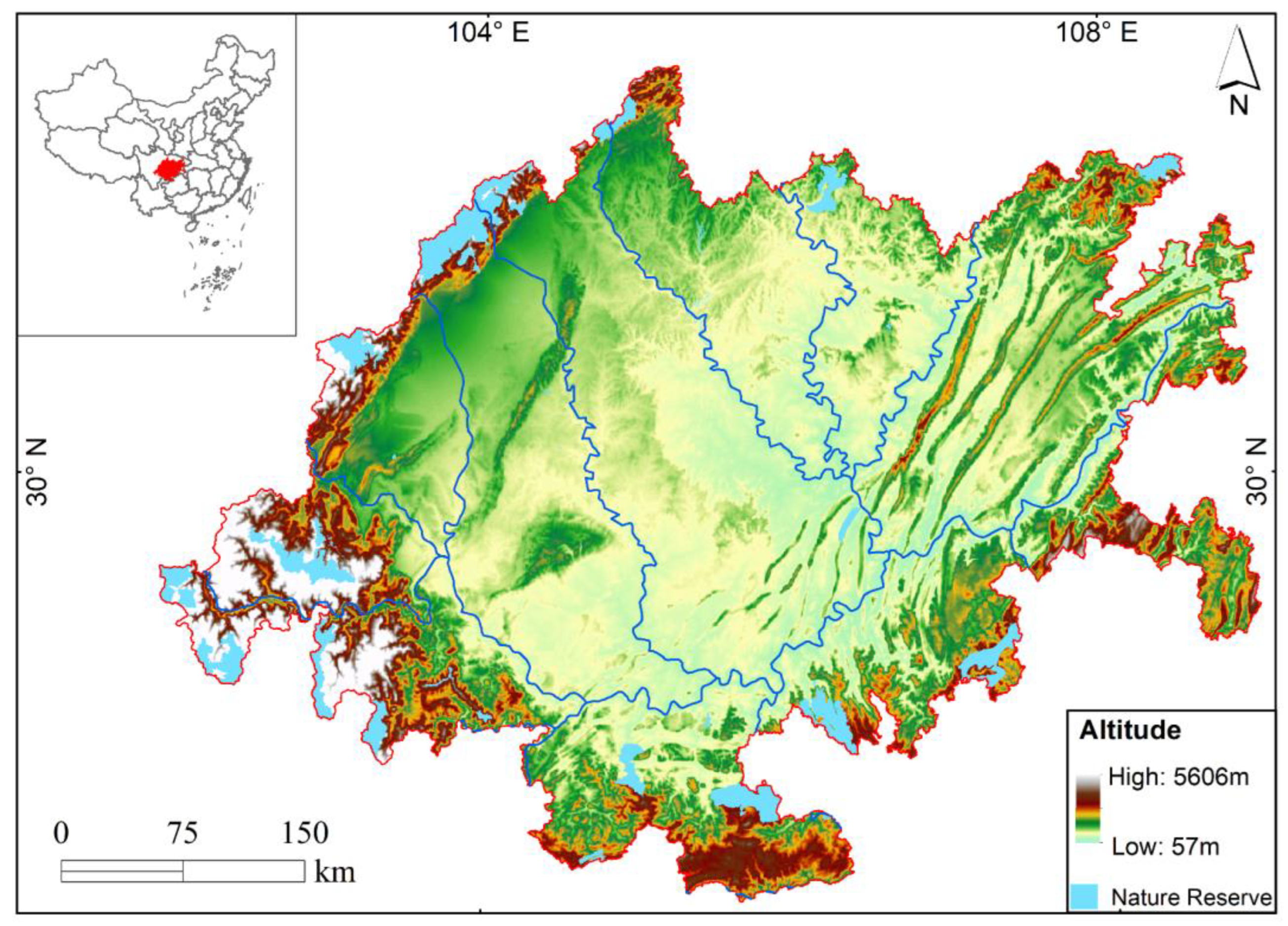
2.1. Study Area
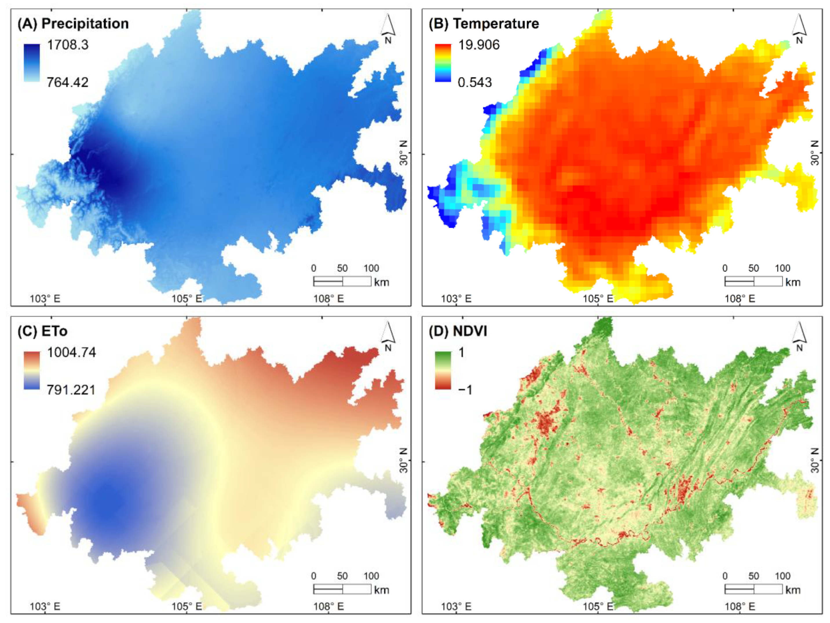
2.2. Data Sources
3. Methods
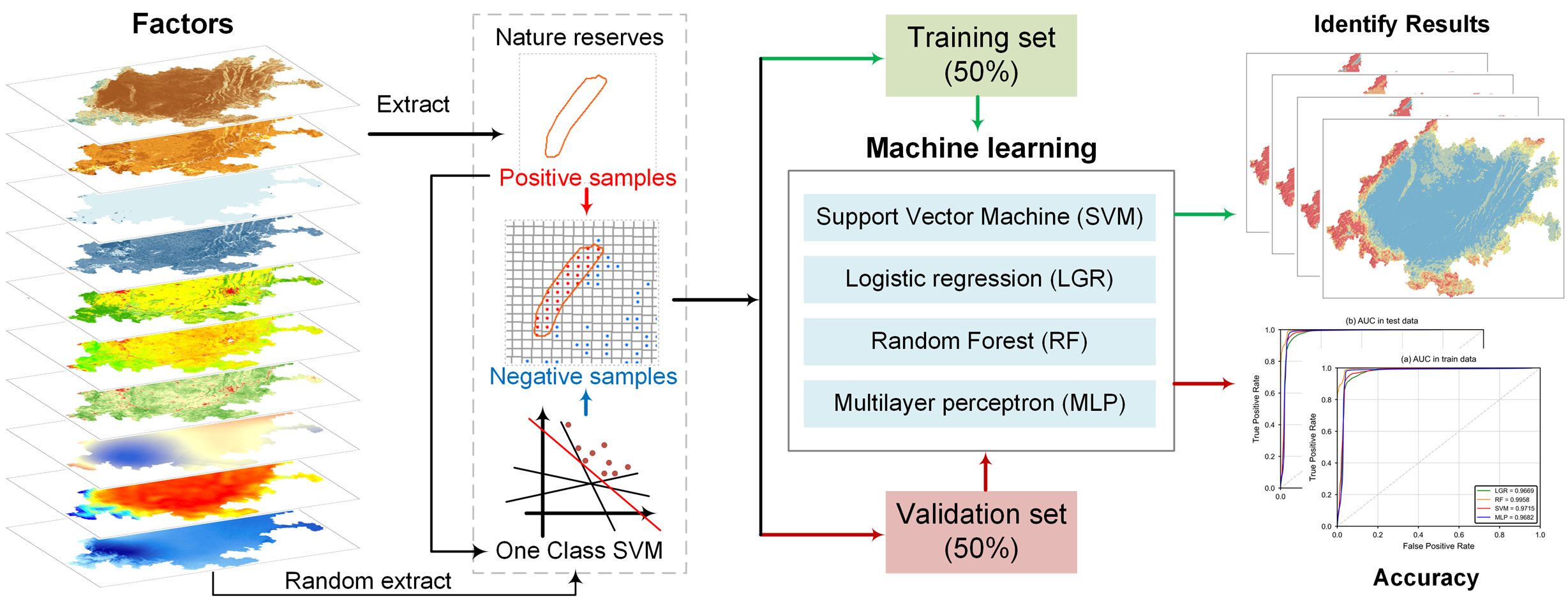
3.1. HCVAs Identification Framework
3.2. Experimental Process and Environment
3.3. Ecosystem Service Functions
3.4. Machine Learning Methods
3.5. One-Class SVM for Samples
3.6. Importance Analysis
3.7. Collinearity Analysis
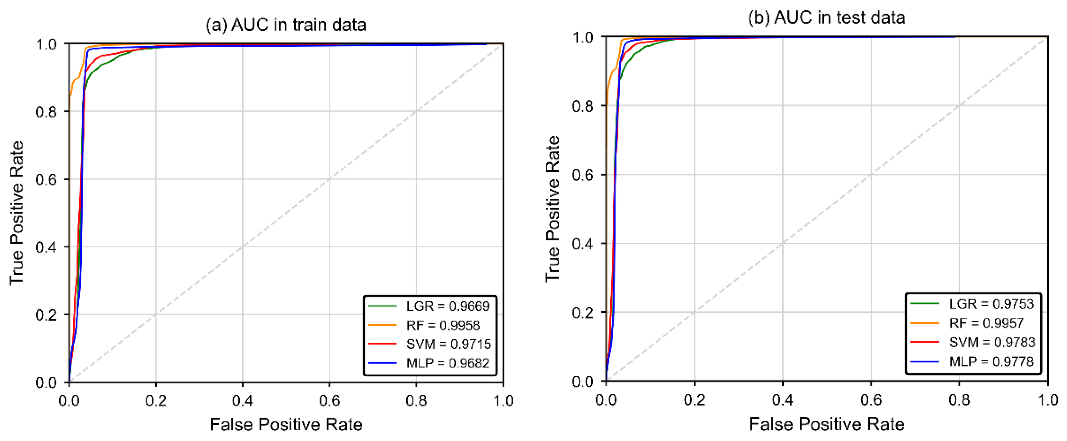
3.8. Accuracy Analysis
4. Results
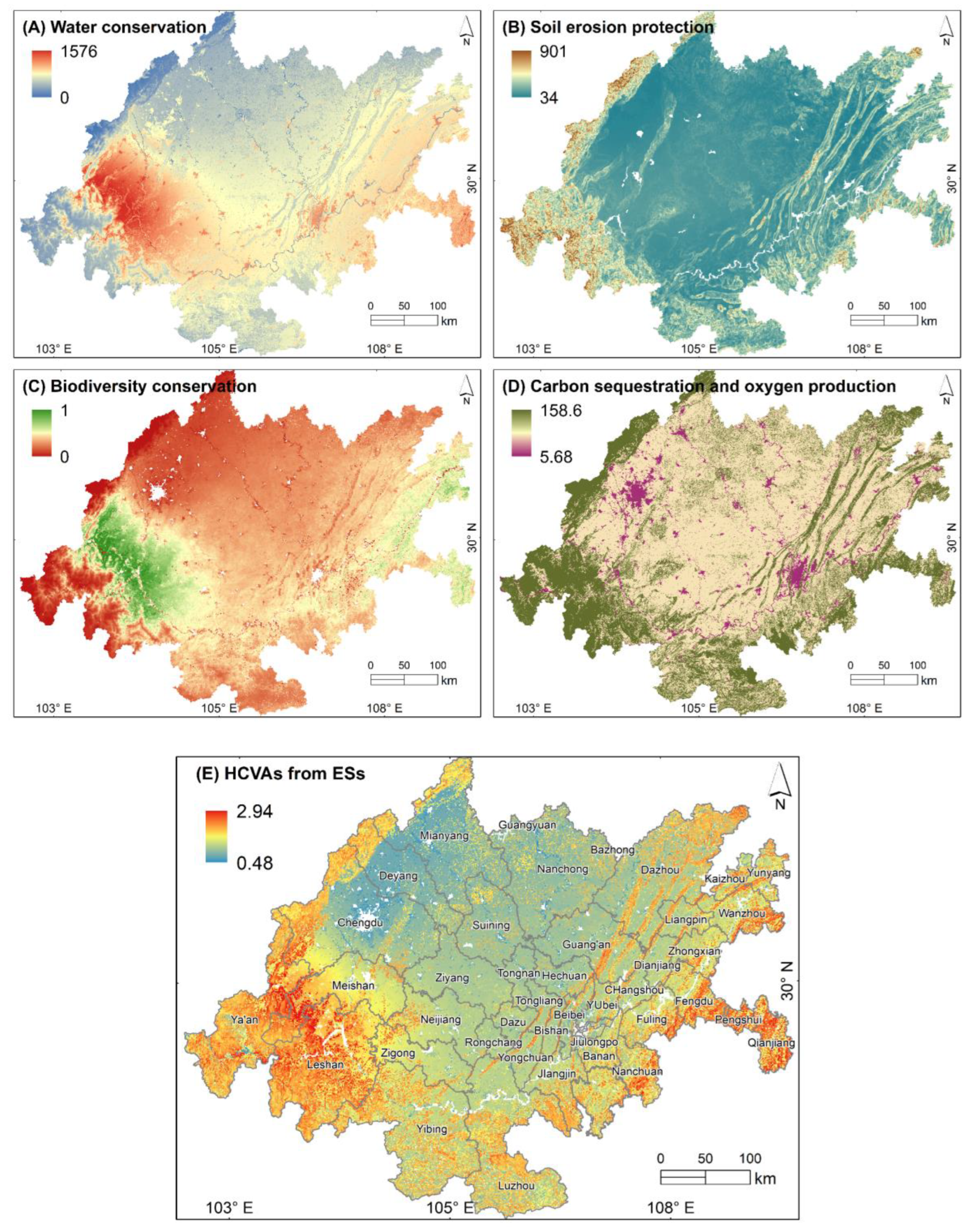
4.1. Evaluation of Ecosystem Services
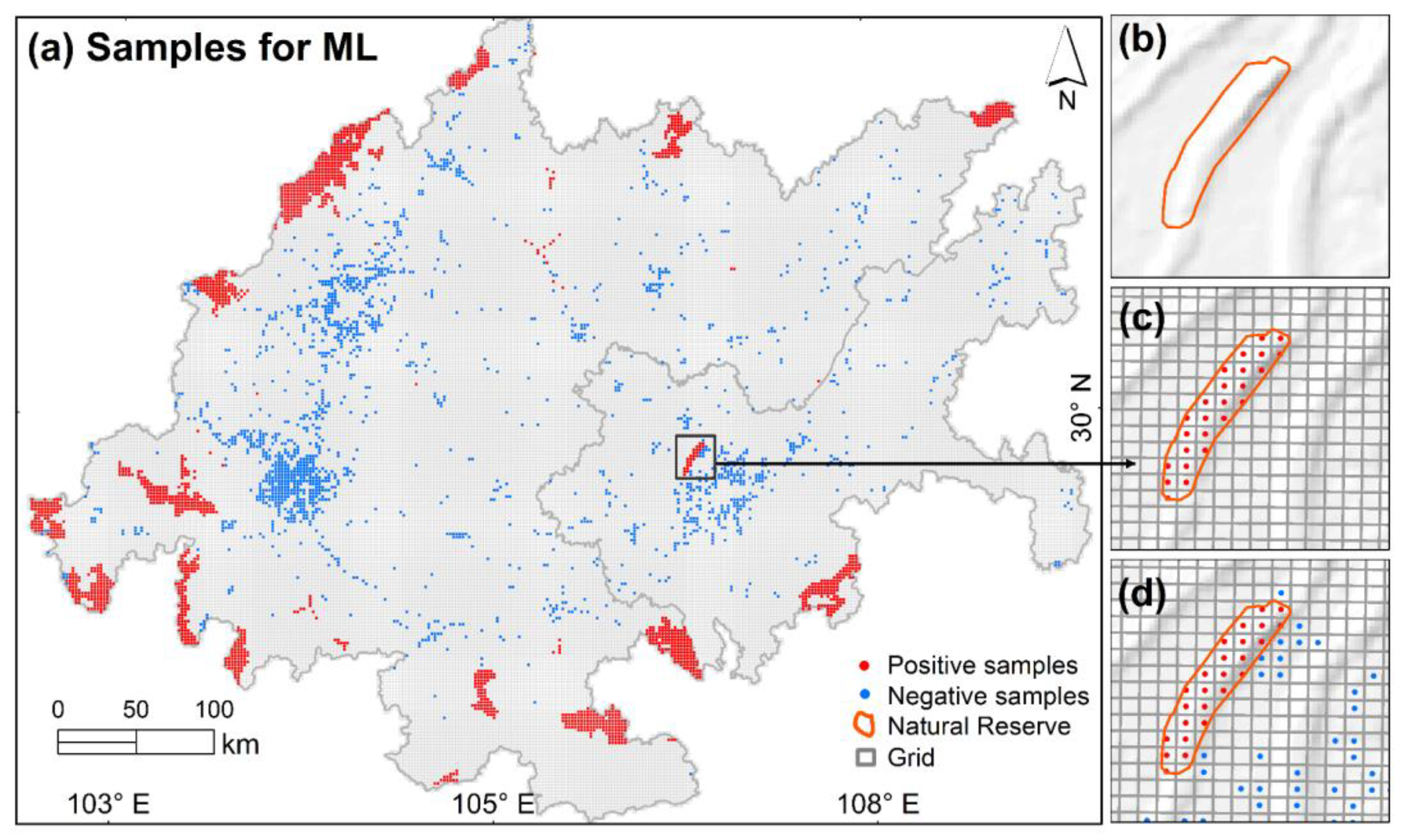
4.2. One-Class SVM Sample Selections
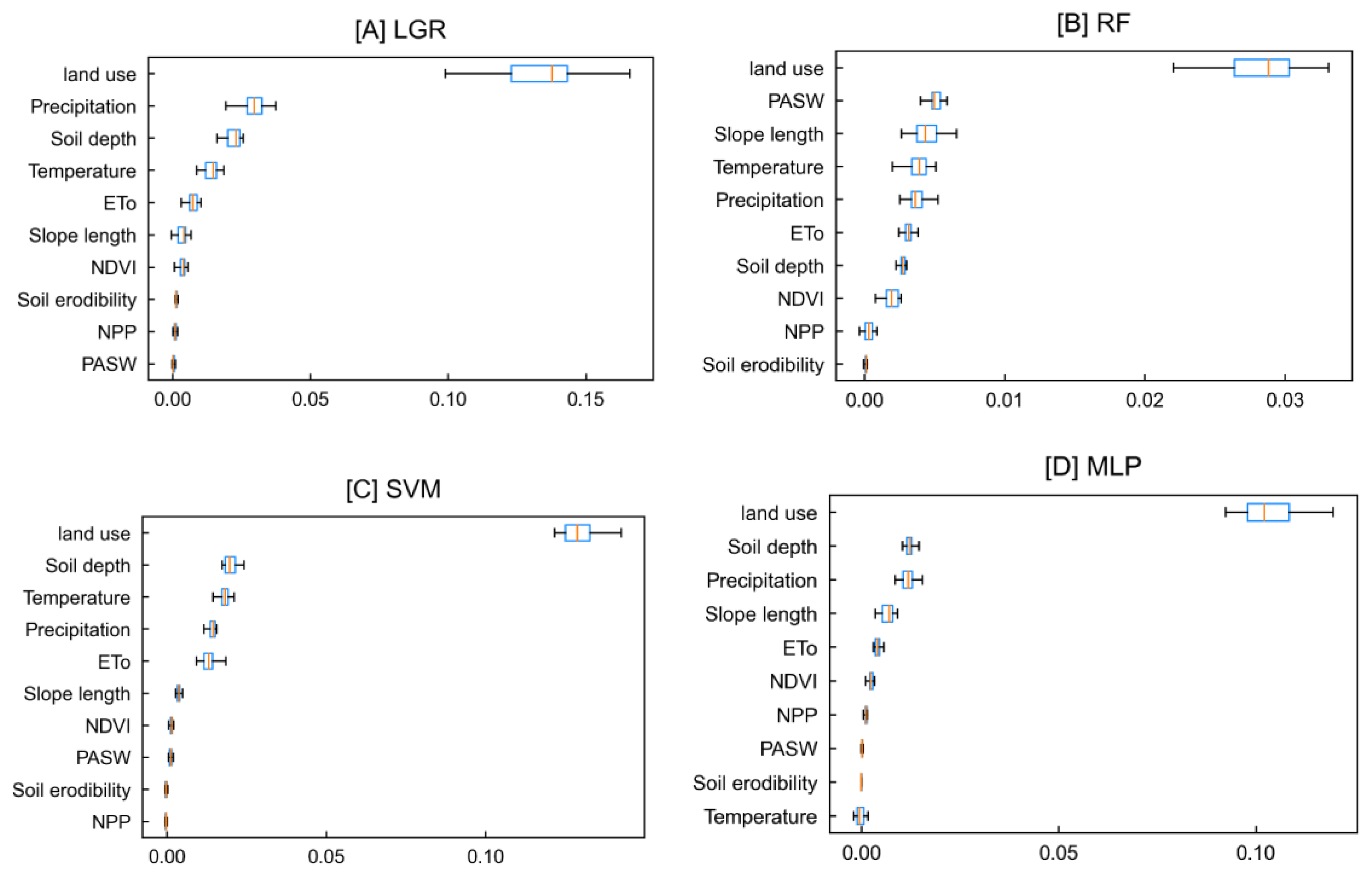
4.3. Factor Selection
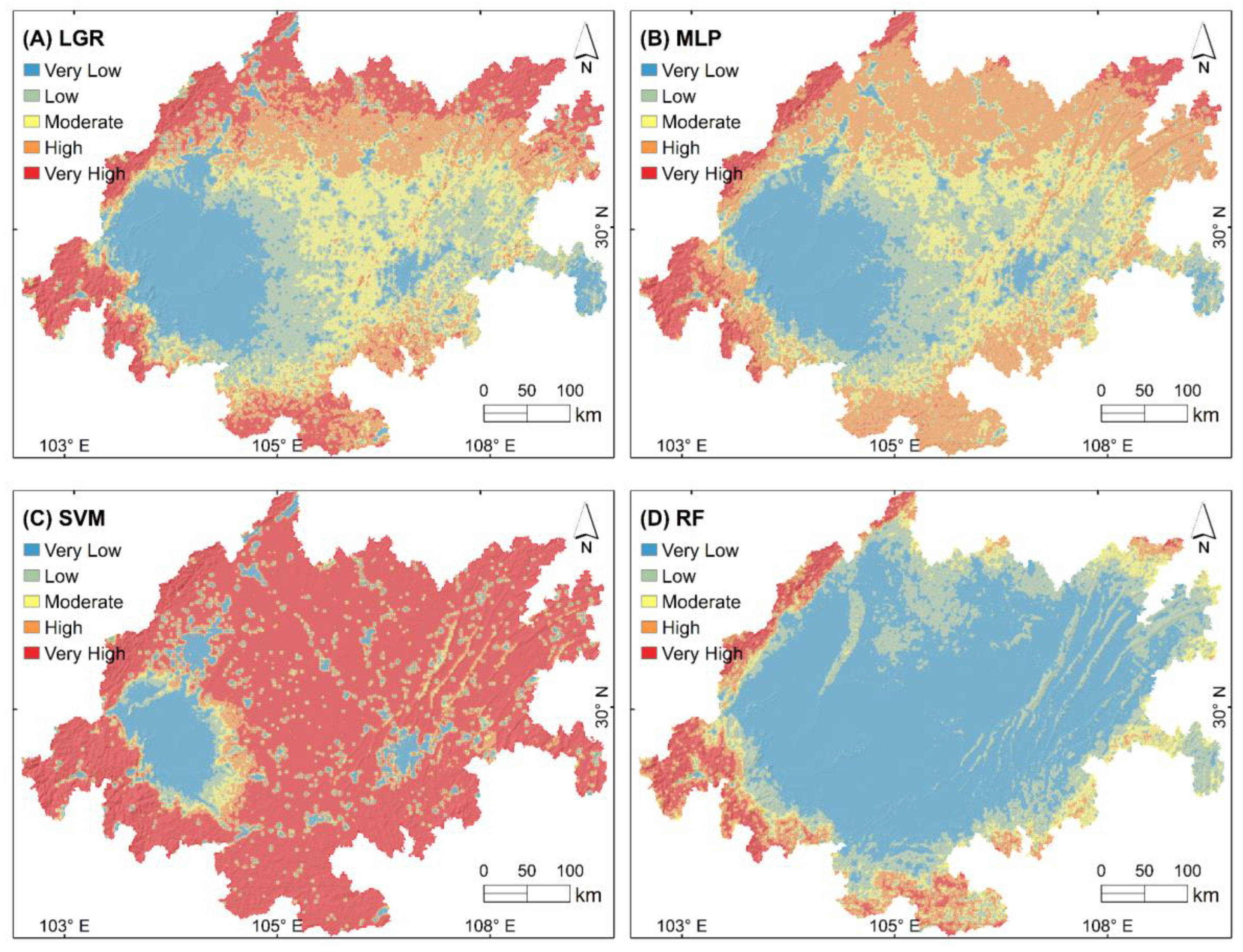
4.4. Prediction Results of ML Models
5. Discussion
5.1. Guidance on the Contribution of ES Factors
5.2. Feasibility of Using ML Models for ERL Identification
6. Conclusions
Author Contributions
Funding
Data Availability Statement
Conflicts of Interest
References
- Millennium Ecosystem Assessment (MEA). Ecosystems and Human Well-Being; Island Press: Washington, DC, USA, 2005; Volume 5. [Google Scholar]
- Steffen, W.; Richardson, K.; Rockström, J.; Cornell, S.E.; Fetzer, I.; Bennett, E.M.; Biggs, R.; Carpenter, S.R.; de Vries, W.; de Wit, C.A.; et al. Planetary Boundaries: Guiding Human Development on a Changing Planet. Science 2015, 347, 1259855. [Google Scholar] [CrossRef] [PubMed]
- Ouyang, X.; Tang, L.; Wei, X.; Li, Y. Spatial Interaction between Urbanization and Ecosystem Services in Chinese Urban Agglomerations. Land Use Policy 2021, 109, 105587. [Google Scholar] [CrossRef]
- Bai, Y.; Wong, C.P.; Jiang, B.; Hughes, A.C.; Wang, M.; Wang, Q. Developing China’s Ecological Redline Policy Using Ecosystem Services Assessments for Land Use Planning. Nat. Commun. 2018, 9, 3034. [Google Scholar] [CrossRef]
- Chen, D.; Pan, Y.; Jin, X.; Du, H.; Li, M.; Jiang, P. The Delineation of Ecological Redline Area for Catchment Sustainable Management from the Perspective of Ecosystem Services and Social Needs: A Case Study of the Xiangjiang Watershed, China. Ecol. Indic. 2021, 121, 107130. [Google Scholar] [CrossRef]
- Gao, J.; Zou, C.; Zhang, K.; Xu, M.; Wang, Y. The Establishment of Chinese Ecological Conservation Redline and Insights into Improving International Protected Areas. J. Environ. Manag. 2020, 264, 110505. [Google Scholar] [CrossRef]
- Li, Z.; Liu, Y.; Zeng, H. Application of the MaxEnt Model in Improving the Accuracy of Ecological Red Line Identification: A Case Study of Zhanjiang, China. Ecol. Indic. 2022, 137, 108767. [Google Scholar] [CrossRef]
- Huang, F.; Yu, Y.; Feng, T. Hyperspectral Remote Sensing Image Change Detection Based on Tensor and Deep Learning. J. Vis. Commun. Image Represent. 2019, 58, 233–244. [Google Scholar] [CrossRef]
- Wei, R.; Ye, C.; Ge, Y.; Li, Y. An Attention-Constrained Neural Network with Overall Cognition for Landslide Spatial Prediction. Landslides 2022, 19, 1087–1099. [Google Scholar] [CrossRef]
- Ye, C.M.; Wei, R.L.; Ge, Y.G.; Li, Y.; Junior, J.M.; Li, J. GIS-Based Spatial Prediction of Landslide Using Road Factors and Random Forest for Sichuan-Tibet Highway. J. Mt. Sci. 2022, 19, 461–476. [Google Scholar] [CrossRef]
- Wei, R.; Ye, C.; Sui, T.; Ge, Y.; Li, Y.; Li, J. Combining Spatial Response Features and Machine Learning Classifiers for Landslide Susceptibility Mapping. Int. J. Appl. Earth Obs. Geoinf. 2022, 107, 102681. [Google Scholar] [CrossRef]
- Meng, C.; Seo, S.; Cao, D.; Griesemer, S.; Liu, Y. When Physics Meets Machine Learning: A Survey of Physics-Informed Machine Learning. arXiv 2022, arXiv:2203.16797. [Google Scholar] [CrossRef]
- Wäldchen, J.; Mäder, P. Machine Learning for Image Based Species Identification. Methods Ecol. Evol. 2018, 9, 2216–2225. [Google Scholar] [CrossRef]
- Tuia, D.; Kellenberger, B.; Beery, S.; Costelloe, B.R.; Zuffi, S.; Risse, B.; Mathis, A.; Mathis, M.W.; van Langevelde, F.; Burghardt, T.; et al. Perspectives in Machine Learning for Wildlife Conservation. Nat. Commun. 2022, 13, 792. [Google Scholar] [CrossRef] [PubMed]
- Scowen, M.; Athanasiadis, I.N.; Bullock, J.M.; Eigenbrod, F.; Willcock, S. The Current and Future Uses of Machine Learning in Ecosystem Service Research. Sci. Total Environ. 2021, 799, 149263. [Google Scholar] [CrossRef]
- Zhong, S.; Zhang, K.; Bagheri, M.; Burken, J.G.; Gu, A.; Li, B.; Ma, X.; Marrone, B.L.; Ren, Z.J.; Schrier, J.; et al. Machine Learning: New Ideas and Tools in Environmental Science and Engineering. Environ. Sci. Technol. 2021, 55, 12741–12754. [Google Scholar] [CrossRef]
- Pichler, M.; Hartig, F. Machine Learning and Deep Learning—A Review for Ecologists. Methods Ecol. Evol. 2023, 14, 994–1016. [Google Scholar] [CrossRef]
- Greener, J.G.; Kandathil, S.M.; Moffat, L.; Jones, D.T. A Guide to Machine Learning for Biologists. Nat. Rev. Mol. Cell Biol. 2022, 23, 40–55. [Google Scholar] [CrossRef]
- Christin, S.; Hervet, É.; Lecomte, N. Applications for Deep Learning in Ecology. Methods Ecol. Evol. 2019, 10, 1632–1644. [Google Scholar] [CrossRef]
- Zhong, J.; Li, Z.; Sun, Z.; Tian, Y.; Yang, F. The Spatial Equilibrium Analysis of Urban Green Space and Human Activity in Chengdu, China. J. Clean. Prod. 2020, 259, 120754. [Google Scholar] [CrossRef]
- Li, Z.; Yang, F.; Zhong, J.; Zhao, J. Self-Organizing Feature Zoning and Multiple Hotspots Identification of Ecosystem Services: How to Promote Ecological Refined Management of Chengdu-Chongqing Urban Agglomeration. J. Urban Plan. Dev. 2023, 149, 04022049. [Google Scholar] [CrossRef]
- Zhang, H. The Impact of Urban Sprawl on Environmental Pollution: Empirical Analysis from Large and Medium-Sized Cities of China. Int. J. Environ. Res. Public Health 2021, 18, 8650. [Google Scholar] [CrossRef] [PubMed]
- Wang, Z.; Yang, J.; Jiang, J. Urban Sprawl and Haze Pollution: Based on Raster Data of Haze PM2.5 Concentrations in 283 Cities in Mainland China. Front. Environ. Sci. 2022, 10, 983. [Google Scholar] [CrossRef]
- Luo, Q.; Zhou, J.; Li, Z.; Yu, B. Spatial Differences of Ecosystem Services and Their Driving Factors: A Comparation Analysis among Three Urban Agglomerations in China’s Yangtze River Economic Belt. Sci. Total Environ. 2020, 725, 138452. [Google Scholar] [CrossRef]
- Lyu, R.; Clarke, K.C.; Zhang, J.; Feng, J.; Jia, X.; Li, J. Spatial Correlations among Ecosystem Services and Their Socio-Ecological Driving Factors: A Case Study in the City Belt along the Yellow River in Ningxia, China. Appl. Geogr. 2019, 108, 64–73. [Google Scholar] [CrossRef]
- Zhang, Z.; Liu, Y.; Wang, Y.; Liu, Y.; Zhang, Y.; Zhang, Y. What Factors Affect the Synergy and Tradeoff between Ecosystem Services, and How, from a Geospatial Perspective? J. Clean. Prod. 2020, 257, 120454. [Google Scholar] [CrossRef]
- Li, X.; Yu, X.; Wu, K.; Feng, Z.; Liu, Y.; Li, X. Land-Use Zoning Management to Protecting the Regional Key Ecosystem Services: A Case Study in the City Belt along the Chaobai River, China. Sci. Total Environ. 2021, 762, 143167. [Google Scholar] [CrossRef] [PubMed]
- Chen, D.; Jiang, P.; Li, M. Assessing Potential Ecosystem Service Dynamics Driven by Urbanization in the Yangtze River Economic Belt, China. J. Environ. Manag. 2021, 292, 112734. [Google Scholar] [CrossRef]
- Zhang, X.; Zhang, G.; Long, X.; Zhang, Q.; Liu, D.; Wu, H.; Li, S. Identifying the Drivers of Water Yield Ecosystem Service: A Case Study in the Yangtze River Basin, China. Ecol. Indic. 2021, 132, 108304. [Google Scholar] [CrossRef]
- Tonghui, M.; Cai, L.; Guangchun, L. The Spatial Overlapping Analysis for China’s Natural Protected Area and Countermeasures for the Optimization and Integration of Protected Area System. Biodivers. Sci. 2019, 27, 758. [Google Scholar] [CrossRef]
- Dou, J.; Yunus, A.P.; Merghadi, A.; Shirzadi, A.; Nguyen, H.; Hussain, Y.; Avtar, R.; Chen, Y.; Pham, B.T.; Yamagishi, H. Different Sampling Strategies for Predicting Landslide Susceptibilities Are Deemed Less Consequential with Deep Learning. Sci. Total Environ. 2020, 720, 137320. [Google Scholar] [CrossRef]
- Li, M.; Liang, D.; Xia, J.; Song, J.; Cheng, D.; Wu, J.; Cao, Y.; Sun, H.; Li, Q. Evaluation of Water Conservation Function of Danjiang River Basin in Qinling Mountains, China Based on InVEST Model. J. Environ. Manag. 2021, 286, 112212. [Google Scholar] [CrossRef]
- Spanò, M.; Leronni, V.; Lafortezza, R.; Gentile, F. Are Ecosystem Service Hotspots Located in Protected Areas? Results from a Study in Southern Italy. Environ. Sci. Policy 2017, 73, 52–60. [Google Scholar] [CrossRef]
- Taner San, B. An Evaluation of SVM Using Polygon-Based Random Sampling in Landslide Susceptibility Mapping: The Candir Catchment Area (Western Antalya, Turkey). Int. J. Appl. Earth Obs. Geoinf. 2014, 26, 399–412. [Google Scholar] [CrossRef]
- Li, S.; Liu, Y.; Yang, H.; Yu, X.; Zhang, Y.; Wang, C. Integrating Ecosystem Services Modeling into Effectiveness Assessment of National Protected Areas in a Typical Arid Region in China. J. Environ. Manag. 2021, 297, 113408. [Google Scholar] [CrossRef] [PubMed]
- Liao, G.; He, P.; Gao, X.; Lin, Z.; Fang, C.; Zhou, W.; Xu, C.; Deng, L. Identifying Critical Area of Ecosystem Service Supply and Demand at Different Scales Based on Spatial Heterogeneity Assessment and SOFM Neural Network. Front. Environ. Sci. 2021, 9, 714874. [Google Scholar] [CrossRef]
- Zhao, M.; He, Z.; Du, J.; Chen, L.; Lin, P.; Fang, S. Assessing the Effects of Ecological Engineering on Carbon Storage by Linking the CA-Markov and InVEST Models. Ecol. Indic. 2019, 98, 29–38. [Google Scholar] [CrossRef]
- Li, K.; Cao, J.; Adamowski, J.F.; Biswas, A.; Zhou, J.; Liu, Y.; Zhang, Y.; Liu, C.; Dong, X.; Qin, Y. Assessing the Effects of Ecological Engineering on Spatiotemporal Dynamics of Carbon Storage from 2000 to 2016 in the Loess Plateau Area Using the InVEST Model: A Case Study in Huining County, China. Environ. Dev. 2021, 39, 100641. [Google Scholar] [CrossRef]
- Haas, J.; Ban, Y. Mapping and Monitoring Urban Ecosystem Services Using Multitemporal High-Resolution Satellite Data. IEEE J. Sel. Top. Appl. Earth Obs. Remote Sens. 2017, 10, 669–680. [Google Scholar] [CrossRef]
- Hu, X.; Luo, H.; Guo, M.; Wang, J. Ecological Technology Evaluation Model and Its Application Based on Logistic Regression. Ecol. Indic. 2022, 136, 108641. [Google Scholar] [CrossRef]
- Mandal, I.; Pal, S. Assessing the Impact of Ecological Insecurity on Ecosystem Service Value in Stone Quarrying and Crushing Dominated Areas. Environ. Dev. Sustain. 2022, 24, 11760–11784. [Google Scholar] [CrossRef]
- Huang, N.; Lu, G.; Xu, D. A Permutation Importance-Based Feature Selection Method for Short-Term Electricity Load Forecasting Using Random Forest. Energies 2016, 9, 767. [Google Scholar] [CrossRef]
- Vidal-Espitia, U.; Serrano-Rubio, J.P.; Ruiz, M.D.M.; Herrera-Guzman, R. Cloud Landscape Images Segmentation Using Artificial Neural Networks and Amazon Web Services for Ecological Applications. In Proceedings of the 2021 IEEE International Conference on Systems, Man, and Cybernetics (SMC), Melbourne, Australia, 17–20 October 2021; pp. 2063–2068. [Google Scholar] [CrossRef]
- Wang, J.; Zhang, Q.; Gou, T.; Mo, J.; Wang, Z.; Gao, M. Spatial-Temporal Changes of Urban Areas and Terrestrial Carbon Storage in the Three Gorges Reservoir in China. Ecol. Indic. 2018, 95, 343–352. [Google Scholar] [CrossRef]
- Ye, C.; Tang, R.; Wei, R.; Guo, Z.; Zhang, H. Generating Accurate Negative Samples for Landslide Susceptibility Mapping: A Combined Self-Organizing-Map and One-Class SVM Method. Front. Earth Sci. 2023, 10, 2049. [Google Scholar] [CrossRef]
- Li, J.; Fan, G.; He, Y. Predicting the Current and Future Distribution of Three Coptis Herbs in China under Climate Change Conditions, Using the MaxEnt Model and Chemical Analysis. Sci. Total Environ. 2020, 698, 134141. [Google Scholar] [CrossRef] [PubMed]
- Smeraldo, S.; Bosso, L.; Salinas-Ramos, V.B.; Ancillotto, L.; Sánchez-Cordero, V.; Gazaryan, S.; Russo, D. Generalists yet Different: Distributional Responses to Climate Change May Vary in Opportunistic Bat Species Sharing Similar Ecological Traits. Mammal Rev. 2021, 51, 571–584. [Google Scholar] [CrossRef]
- Merghadi, A.; Yunus, A.P.; Dou, J.; Whiteley, J.; ThaiPham, B.; Bui, D.T.; Avtar, R.; Abderrahmane, B. Machine Learning Methods for Landslide Susceptibility Studies: A Comparative Overview of Algorithm Performance. Earth-Sci. Rev. 2020, 207, 103225. [Google Scholar] [CrossRef]
- Altmann, A.; Toloşi, L.; Sander, O.; Lengauer, T. Permutation Importance: A Corrected Feature Importance Measure. Bioinformatics 2010, 26, 1340–1347. [Google Scholar] [CrossRef] [PubMed]
- Bergstra, J.; Bengio, Y. Random Search for Hyper-Parameter Optimization. J. Mach. Learn. Res. 2012, 13, 281–305. [Google Scholar]
- Alemu I, J.B.; Richards, D.R.; Gaw, L.Y.F.; Masoudi, M.; Nathan, Y.; Friess, D.A. Identifying Spatial Patterns and Interactions among Multiple Ecosystem Services in an Urban Mangrove Landscape. Ecol. Indic. 2021, 121, 107042. [Google Scholar] [CrossRef]
- Radeloff, V.C.; Dubinin, M.; Coops, N.C.; Allen, A.M.; Brooks, T.M.; Clayton, M.K.; Costa, G.C.; Graham, C.H.; Helmers, D.P.; Ives, A.R.; et al. The Dynamic Habitat Indices (DHIs) from MODIS and Global Biodiversity. Remote Sens. Environ. 2019, 222, 204–214. [Google Scholar] [CrossRef]
- Chen, B.; Li, Z.; Zhang, C.; Ding, M.; Zhu, W.; Zhang, S.; Han, B.; Du, J.; Cao, Y.; Zhang, C.; et al. Wide Area Detection and Distribution Characteristics of Landslides along Sichuan Expressways. Remote Sens. 2022, 14, 3431. [Google Scholar] [CrossRef]
- Bao, F.; Qiu, J. Ecological Vulnerability Assessment of the Ya’an-Qamdo Section along the Southern Route of the Sichuan-Tibet Transportation Corridor. J. Mt. Sci. 2022, 19, 2202–2213. [Google Scholar] [CrossRef]
- Huang, A.; Xu, Y.; Sun, P.; Zhou, G.; Liu, C.; Lu, L.; Xiang, Y.; Wang, H. Land Use/Land Cover Changes and Its Impact on Ecosystem Services in Ecologically Fragile Zone: A Case Study of Zhangjiakou City, Hebei Province, China. Ecol. Indic. 2019, 104, 604–614. [Google Scholar] [CrossRef]
- Berdugo, M.; Delgado-Baquerizo, M.; Soliveres, S.; Hernández-Clemente, R.; Zhao, Y.; Gaitán, J.J.; Gross, N.; Saiz, H.; Maire, V.; Lehman, A.; et al. Global Ecosystem Thresholds Driven by Aridity. Science 2020, 367, 787–790. [Google Scholar] [CrossRef]
- Wang, Z.; Guo, J.; Ling, H.; Han, F.; Kong, Z.; Wang, W. Function Zoning Based on Spatial and Temporal Changes in Quantity and Quality of Ecosystem Services under Enhanced Management of Water Resources in Arid Basins. Ecol. Indic. 2022, 137, 108725. [Google Scholar] [CrossRef]
- Hu, T.; Peng, J.; Liu, Y.; Wu, J.; Li, W.; Zhou, B. Evidence of Green Space Sparing to Ecosystem Service Improvement in Urban Regions: A Case Study of China’s Ecological Red Line Policy. J. Clean. Prod. 2020, 251, 119678. [Google Scholar] [CrossRef]
- Chunye, W.; Delu, P. Zoning of Hangzhou Bay Ecological Red Line Using GIS-Based Multi-Criteria Decision Analysis. Ocean. Coast. Manag. 2017, 139, 42–50. [Google Scholar] [CrossRef]
- Zhang, H.; Pang, Q.; Hua, Y.; Li, X.; Liu, K. Linking Ecological Red Lines and Public Perceptions of Ecosystem Services to Manage the Ecological Environment: A Case Study in the Fenghe River Watershed of Xi’an. Ecol. Indic. 2020, 113, 106218. [Google Scholar] [CrossRef]
- Lin, J.; Li, X. Large-Scale Ecological Red Line Planning in Urban Agglomerations Using a Semi-Automatic Intelligent Zoning Method. Sustain. Cities Soc. 2019, 46, 101410. [Google Scholar] [CrossRef]
- Lu, W.H.; Liu, J.; Xiang, X.Q.; Song, W.L.; McIlgorm, A. A Comparison of Marine Spatial Planning Approaches in China: Marine Functional Zoning and the Marine Ecological Red Line. Mar. Policy 2015, 62, 94–101. [Google Scholar] [CrossRef]
- Xu, X.; Yang, G.; Tan, Y. Identifying Ecological Red Lines in China’s Yangtze River Economic Belt: A Regional Approach. Ecol. Indic. 2019, 96, 635–646. [Google Scholar] [CrossRef]


| Factors | Data | Resolution/m | |
|---|---|---|---|
| Climate | Precipitation | Dataset of annual rainfall in Tibet 1 | 1000 |
| Temperature | TerraClimate 2 | 1000 | |
| Topography | ETo | China’s Surface climate data 3 | 1000 |
| Elevation | SRTM Digital Elevation 30 m 2 | 90 | |
| Slope length | SRTM Digital Elevation 30 m 2 | 90 | |
| Vegetation | NDVI | NDVI Landsat 8 8-Day NDVI Composite 2 | 250 |
| NPP | MOD17A2/Terra Net Photosynthesis 8-day L4 2 | 250 | |
| Soil | Soil depth | World Soil Database 4 | 1000 |
| PASW | World Soil Database 4 | 1000 | |
| Soil erodibility | World Soil Database 4 | 500 | |
| Land cover | Land use | FROM-GLC10 5 | 30 |
| Ecosystem Services | Formulae | Parameters |
|---|---|---|
| Water conservation (WC) | is the annual water production depth of grid x (mm); is the average annual precipitation; is the actual evapotranspiration (mm); is the annual potential evapotranspiration (mm); is the vegetation evapotranspiration coefficient; is the reference crop evapotranspiration; is the seasonal parameter; is the effective water content of soil (mm). | |
| Soil erosion protection (Spro) | | is the soil conservation (t·hm−2·a−1); is the potential soil erosion (t·hm−2·a−1); is the actual soil erosion (t·hm−2·a−1); is the rainfall erosion factor (MJ·mm·hm−2·h−1·a−1); is the soil erodibility (t·hm−2·h·hm−2·MJ−1·mm−1); is the gradient slope and slope length; is the vegetation cover management factor; is the water and soil conservation measures. |
| Biodiversity conservation (Sbio) | is the net primary productivity gC/(m2·year); is the average annual precipitation; is the annual average temperature; is the altitude. | |
| Carbon storage and oxygen production (CSOP) | | is the aboveground unit carbon sequestration; is the underground unit carbon sequestration; is the soil unit carbon sequestration; is the dead organisms’ unit carbon; is the Carbon density of land use type ; is the area of land use ; |
| ML | Formulae | Parameters |
|---|---|---|
| Support Vector Machine (SVM) | | is the edge distance; are positive and negative samples; is the norm of the hyperplane normal vector; is the distance bias. is the Lagrange coefficient. |
| Logistic regression (LGR) | | where is the bias; are regression coefficients; are explanatory variables. |
| Random forest (RF) | | is the Gini impurity; is the number of positive samples at node ; is the number of eigenvectors used for training; is the number of values belonging to class ; is the number of values at node . |
| Multilayer perceptron (MLP) | | are inputs; and are the weights and bias between neurons; is the activation function; is the number of network layers; is the number of input samples; and are the true value and predicted value of the -th sample, respectively. |
| Factors | TOL | VIF | p Value | Std Err |
|---|---|---|---|---|
| DEM | 0.068 | 14.709 | - | - |
| Temperature | 0.226 | 4.424 | 0.094 | 0.029 |
| NDVI | 0.266 | 3.766 | 0 | 0.037 |
| NPP | 0.282 | 3.546 | 0 | 0.048 |
| Slope length | 0.340 | 2.941 | 0 | 0.027 |
| Precipitation | 0.357 | 2.802 | 0.098 | 0.024 |
| Land use | 0.416 | 2.404 | 0 | 0.015 |
| ETo | 0.576 | 1.737 | 0 | 0.020 |
| Soil depth | 0.775 | 1.289 | 0 | 0.016 |
| PASW | 0.838 | 1.194 | 0 | 0.020 |
| Soil erodibility | 0.908 | 1.101 | 0 | 0.030 |
| TP | TN | FP | FN | AUC | OA | Pre | Sen | Spe | F1 | kappa | |
|---|---|---|---|---|---|---|---|---|---|---|---|
| LGR | 843 | 823 | 52 | 48 | 0.975 | 0.943 | 0.942 | 0.946 | 0.941 | 0.944 | 0.887 |
| RF | 885 | 839 | 36 | 6 | 0.996 | 0.976 | 0.961 | 0.993 | 0.959 | 0.977 | 0.952 |
| SVM | 857 | 830 | 45 | 34 | 0.978 | 0.955 | 0.950 | 0.962 | 0.949 | 0.956 | 0.911 |
| MLP | 831 | 847 | 28 | 60 | 0.978 | 0.950 | 0.967 | 0.933 | 0.968 | 0.950 | 0.900 |
Disclaimer/Publisher’s Note: The statements, opinions and data contained in all publications are solely those of the individual author(s) and contributor(s) and not of MDPI and/or the editor(s). MDPI and/or the editor(s) disclaim responsibility for any injury to people or property resulting from any ideas, methods, instructions or products referred to in the content. |
© 2024 by the authors. Licensee MDPI, Basel, Switzerland. This article is an open access article distributed under the terms and conditions of the Creative Commons Attribution (CC BY) license (https://creativecommons.org/licenses/by/4.0/).
Share and Cite
Deng, J.; Xie, Y.; Wei, R.; Ye, C.; Wang, H. Application of Machine Learning in Ecological Red Line Identification: A Case Study of Chengdu–Chongqing Urban Agglomeration. Diversity 2024, 16, 300. https://doi.org/10.3390/d16050300
Deng J, Xie Y, Wei R, Ye C, Wang H. Application of Machine Learning in Ecological Red Line Identification: A Case Study of Chengdu–Chongqing Urban Agglomeration. Diversity. 2024; 16(5):300. https://doi.org/10.3390/d16050300
Chicago/Turabian StyleDeng, Juan, Yu Xie, Ruilong Wei, Chengming Ye, and Huajun Wang. 2024. "Application of Machine Learning in Ecological Red Line Identification: A Case Study of Chengdu–Chongqing Urban Agglomeration" Diversity 16, no. 5: 300. https://doi.org/10.3390/d16050300
APA StyleDeng, J., Xie, Y., Wei, R., Ye, C., & Wang, H. (2024). Application of Machine Learning in Ecological Red Line Identification: A Case Study of Chengdu–Chongqing Urban Agglomeration. Diversity, 16(5), 300. https://doi.org/10.3390/d16050300