
Heat Bath in a Quantum Circuit


1
Pico Group, QTF Centre of Excellence, Department of Applied Physics, Aalto University, P.O. Box 15100, FI-00076 Aalto, Finland
2
QTF Centre of Excellence, Department of Physics, Faculty of Science, University of Helsinki, FI-00014 Helsinki, Finland
*
Author to whom correspondence should be addressed.
Entropy 2024, 26(5), 429; https://doi.org/10.3390/e26050429
Submission received: 25 April 2024
/
Revised: 9 May 2024
/
Accepted: 10 May 2024
/
Published: 17 May 2024
(This article belongs to the Special Issue Advances in Quantum Thermodynamics)
Abstract
:We discuss the concept and realization of a heat bath in solid state quantum systems. We demonstrate that, unlike a true resistor, a finite one-dimensional Josephson junction array or analogously a transmission line with non-vanishing frequency spacing, commonly considered as a reservoir of a quantum circuit, does not strictly qualify as a Caldeira–Leggett type dissipative environment. We then consider a set of quantum two-level systems as a bath, which can be realized as a collection of qubits. We show that only a dense and wide distribution of energies of the two-level systems can secure long Poincare recurrence times characteristic of a proper heat bath. An alternative for this bath is a collection of harmonic oscillators, for instance, in the form of superconducting resonators.
1. Introduction
The question of thermalization in closed quantum systems and the nature of thermal reservoirs are topics of considerable interest [1,2,3,4,5,6,7]. However, experimental realizations, in particular, in the solid-state domain are largely missing [4,8]. In this paper, we compare different types of reservoirs that can be realized in the context of superconducting quantum circuits. An ideal heat bath is a resistor [9,10,11,12,13,14,15], which can be realized in a straightforward way. However, mainly because of the compatibility of the fabrication processes, the circuit QED community typically prefers to mimic resistors or simply to produce high-impedance environments by arrays of Josephson junctions or superconducting cavities [16,17,18,19,20,21,22,23,24]. The advantages of a physical resistor in the form of a metal film are that it has a truly gapless and smooth absorption spectrum, and on the practical side its temperature can be probed by a standard thermometer [25]. A one-dimensional Josephson junction array, on the contrary, although acting as a high impedance environment [26,27], presents well-defined resonances in its absorption spectrum up to the plasma frequency and purely capacitive behavior above it and cannot thus be considered rigorously as a resistor. Experiments on multimode cavities support our conclusion, as they exhibit periodic recoveries of the qubit coupled to them [28]. In order to realize a Caldeira–Leggett type true reservoir [29,30] out of superconducting elements, we propose an ensemble of qubits or -resonators with a distribution of energies among them.
2. Basic Properties of Resonators and Josephson Arrays
We start with an elementary classical analysis of a one-dimensional Josephson junction array (see Figure 1a), which can be presented in a linearized form by a chain of parallel elements for the junctions, with a ground capacitance between two of them, as in Figure 1b. Assuming a long array, we can write for voltage on island k and current , through the corresponding junction,
Here, with , is the angular frequency of driving, is the plasma frequency of the junction, and is the current through the k:th junction. One can solve these equations with different terminations of the array. One finds the dispersion relation of the angular frequencies for infinite impedance at
where, for an array of N junctions, for a shorted termination, and for an open line [20] (These frequencies practically coincide with those obtained by exact diagonalization of an array of arbitrary length and those from numerical results for , which is the usual regime). This is the functional dependence of the dispersion relation used in fitting the data, e.g., in Refs. [22,24], and it is depicted in Figure 1c for two different values of , one for the pure transmission line and the other for . Figure 1d–f shows the modulus of the frequency dependent impedance of an array calculated numerically for . We conclude that such an array can hardly be considered to be a resistor. The resonant absorption at frequencies corresponding to Equation (2) is presented in experiments as well [22,24]. At frequencies above , there are no more modes, and the impedance is purely capacitive, with impedance asymptotically at high frequencies (see Figure 1f).
3. Resonators and Josephson Arrays as Environment: Model
We next analyze the energy exchange between the system (here, a qubit) and a reservoir to assess whether the latter qualifies as a thermal bath. In general, an ideal array presents a reactive element that cannot dissipate the energy. Such a conclusion can be drawn for instance by analyzing the population of a qubit coupled to the array. To be concrete, we follow the model in Refs. [28,31] and consider a qubit with energy coupled to a bath of N states, with the energy of the j:th one equal to . The Hamiltonian of the whole system and bath is given by
where for the qubit with eigenstates (ground) and (excited), and is the creation (annihilation) operator of the environment modes. The non-interacting Hamiltonian is . The parameters represent the coupling of the qubit with each state in the environment for the perturbation, which reads in the interaction picture with respect to as
The basis that we use is formed of the states of the system and environment as , where the first entrance refers to the qubit and from the second on to each of the N states in the bath. In what follows, we apply this model to both a multimode cavity and spins as environment. We choose the initial state of the whole system (qubit and environment) as . This corresponds to the ground state of the environment (zero temperature, ) but with the qubit excited. The assumption of such a vacuum initial state is justified because, in typical experiments on superconducting qubits, the energy of the qubit is of the order of 1 K, whereas the temperature of the experiment is about 0.01 K. Since, especially in the weak coupling case, the qubit interacts mainly with degenerate states, the assumption of no excitations initially is a good one. We solve the Schrödinger equation in the interaction picture to find the time evolution of the state of the whole system, . In the given basis, the amplitudes are then governed by
With the initial conditions and for , i.e., with state , we find
In the rest of the paper, we integrate these equations numerically for the given set of couplings and frequencies.
4. Results on the Qubit + Resonator Environment Dynamics
Returning first to a Josephson junction array or a finite transmission line, we may write the (angular) frequencies of the multimode resonator as (exactly for an transmission line and approximately for the array well below , see Equation (2)), where the spacing is given by the length of the line or array as discussed above for the latter. Furthermore, we assume the standard coupling as , where g is the coupling constant arising, e.g., from the capacitance between the qubit and the resonator [28]. This model, with the system depicted in Figure 2a, demonstrates in the absence of true dissipative elements almost periodic exchange of energy between the qubit and the cavity shown in Figure 2b, where the excited state population of the qubit is depicted against the normalized time . This is in contrast to the exponential decay in the case of a resistor as environment. In this numerical example, we chose and included states in the calculation. This energy spacing approximately mimics the experiment of Ref. [28]. We can see that the revivals are not full, and the energy of the qubit is distributed over many states with energies in the neighborhood of . Zooming in to the short time regime as in Figure 2c, we observe the exponential decay of the population over eight orders of magnitude. A closer analysis of the dynamics yields that the decay in short times is indeed exponential, with a decay rate , following the numerical result of Figure 2c. The other important feature in the dynamics, naturally, is the periodic recoveries of . The first repopulation demonstrates a sharp peak that sets abruptly on at time . We may associate this with the time of flight of a photon with frequency through the transmission line and reflected back; thus, t is proportional to the length of the line or N in the array. In practical circuits, this recovery time falls into a very short nanosecond regime, meaning that the transmission line acts as a bath only for times shorter than this. In Ref. [28], similar results as in Figure 2b were obtained using the input–output theory [32,33]. The results are robust against different terminations of the line. We also tested the dynamics using different initial states of the system, which did not lead to noticeable changes in the recovery time.
5. Heat Bath Formed of Two-Level Systems (Qubits)
As is well known, a set of reactive elements can, however, effectively approximate a dissipative element in the spirit of Caldeira and Leggett [29]. We will next discuss the conditions of forming a heat bath in a solid-state quantum context without actual dissipative building blocks. In particular, we focus on a collection of coupled quantum two-level systems (TLSs), which can, in practice, be formed of Josephson junction based qubits [34] or of unknown structural defects in superconducting circuits [35,36]. A set of harmonic oscillators in the form of superconducting cavities would provide an alternative realization of a Caldeira–Leggett environment. Here, we focus on TLSs. Returning to the archetypal setup, where a central qubit couples to an ensemble of these TLSs, we observe the dynamics of this qubit when initially set to its excited state. We use the same model as above but now with different distributions of energies and couplings of the TLSs. For the sake of clarity of the argument, all the TLSs are again set initially to their ground state, mimicking a zero temperature environment. As we have shown in another context [31], a broad distribution of energies of the TLSs secures the exponential decay of the qubit population in time. This can be seen also analytically, for instance, by standard means re-summing in all orders of perturbation, assuming a large number of uniformly distributed TLS energies. The distribution of energies and couplings of the TLSs is an essential condition for absorbing the energy of the qubit to this bath without recoveries over any practical timescales. In this case, the qubit decays exponentially as
Here, , with , the density of TLSs around , and .
In general, for any distribution of energies and couplings, we find that the qubit amplitude in the excited state is governed by the integro-differential equation
We see immediately that, for the case where all the TLSs have the same energy as the qubit, for all k, and the qubit does not decay, even when the couplings are fully random; however, it oscillates with the population ; i.e., the Poincare recovery time is .
We can generalize the conclusion above for a bath where for arbitrary positive r, meaning detuned equal-energy TLSs in the environment. In this case, Equation (8) leads to , where . satisfies the initial conditions , and . We then have the oscillatory solution
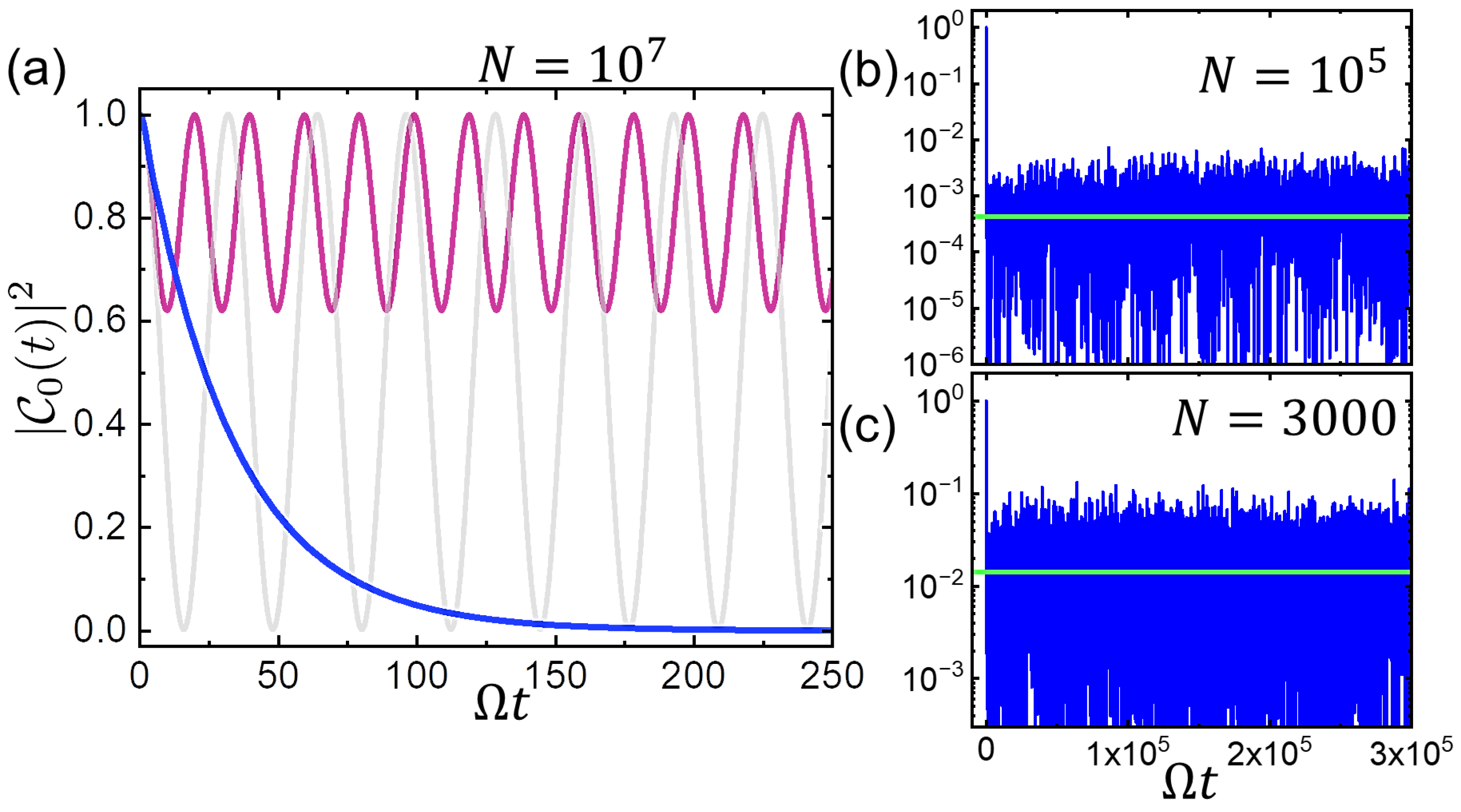
Figure 3a shows the numerically calculated results of for TLSs and for different choices of parameters following closely the analytical results given above. For a uniform distribution of TLS energies in the range , the decay is exponential as described above, whereas for TLSs with identical energies, there are periodic revivals in quantitative agreement with the analytic result. These results serve as a warning sign for models where bath spins are assumed to have equal energies. In Figure 3b,c, we numerically monitor the long time behavior of under the same conditions as in the main frame but with and TLSs with distributed energies and couplings. We see that there are no revivals over this long period of time in both cases, and the long time population follows closely the prediction indicated by the horizontal lines [37]. This result emphasizes the importance of randomness (in couplings and frequencies) to prolong the Poincare recurrence time.
Two possible realizations of such reactive baths can be immediately envisioned. The one that corresponds to our analysis here is that of a qubit coupled to a TLS environment with variable energies: with modern qubits as TLSs, the couplings and energies can be varied almost arbitrarily [34]. One can envison to couple hundreds, perhaps even thousands, of such artificial TLSs to a qubit. A simpler choice could be an ensemble of superconducting resonators with the same idea: here, the tunability is more limited, and instead of TLSs, these resonators work as harmonic oscillators.
6. Summary
In summary, it is possible to form a thermal bath on a chip, avoiding recurrences [38] over any practical time scale, in the spirit of Caldeira and Leggett [29] using just reactive elements. However, a one-dimensional array of Josephson junctions or alternatively a transmission line exhibits periodic recoveries on nanosecond time scales in practical physical circuits for two reasons: first, the energy distribution is not dense, and, equally importantly the coupling is not random but essentially equal () to each state i. Such an environment is thus a heat bath only if it has significant intrinsic dissipation, valid typically for [18,20], or if it is terminated by a resistive element [39]; in this case the termination itself is the bath. A way around to achieve a true bath is to form a network of harmonic oscillators or TLSs with distributed parameters and couple it to the quantum system.
Author Contributions
Conceptualization, J.P.P.; Methodology, B.K.; Formal analysis, J.P.P. and B.K.; Writing—original draft, J.P.P.; Writing—review & editing, B.K. All authors have read and agreed to the published version of the manuscript.
Funding
This work was supported by the Research Council of Finland Grant No. 312057 (Centre of Excellence program) and Grant No. 349601 (THEPOW).
Data Availability Statement
Data are contained within the article.
Acknowledgments
We thank Diego Subero, Charles Marcus, Andrew Cleland, Youpeng Zhong, Vladimir Manucharyan, Alfredo Levy Yeyati, Mikko Möttönen, Arman Alizadeh, Paolo Muratore-Ginanneschi, Vasilii Vadimov, and Angelo Vulpiani for useful discussions.
Conflicts of Interest
The authors declare no conflicts of interest.
References
- Mori, T.; Ikeda, T.N.; Kaminishi, E.; Ueda, M. Thermalization and prethermalization in isolated quantum systems: A theoretical overview. J. Phys. B At. Mol. Opt. Phys. 2018, 51, 112001. [Google Scholar] [CrossRef]
- Nandkishore, R.; Huse, D.A. Many-Body Localization and Thermalization in Quantum Statistical Mechanics. Annu. Rev. Condens. Matter Phys. 2015, 6, 15. [Google Scholar] [CrossRef]
- Zwanzig, R. Nonequilibrium Statistical Mechanics; Oxford University Press: Oxford, UK, 2001. [Google Scholar]
- Reimann, P. Typical fast thermalization processes in closed many-body systems. Nat. Commun. 2016, 7, 10821. [Google Scholar] [CrossRef] [PubMed]
- D’Alessio, L.; Kafri, Y.; Polkovnikov, A.; Rigol, M. From quantum chaos and eigenstate thermalization to statistical mechanics and thermodynamics. Adv. Phys. 2016, 65, 239. [Google Scholar] [CrossRef]
- Popescu, S.; Short, A.; Winter, A. Entanglement and the foundations of statistical mechanics. Nat. Phys. 2006, 2, 754. [Google Scholar] [CrossRef]
- Rigol, M.; Dunjko, V.; Yurovsky, V.; Olshanii, M. Relaxation in a Completely Integrable Many-Body Quantum System: An Ab Initio Study of the Dynamics of the Highly Excited States of 1D Lattice Hard-Core Bosons. Phys. Rev. Lett. 2007, 98, 050405. [Google Scholar] [CrossRef] [PubMed]
- Chen, F.; Sun, Z.; Gong, M.; Zhu, Q.; Zhang, Y.; Wu, Y.; Ye, Y.; Zha, C.; Li, S.; Guo, S.; et al. Observation of Strong and Weak Thermalization in a Superconducting Quantum Processor. Phys. Rev. Lett. 2021, 127, 020602. [Google Scholar] [CrossRef] [PubMed]
- Kuzmin, L.S.; Haviland, D.B. Observation of the Bloch oscillations in an ultrasmall Josephson junction. Phys. Rev. Lett. 1991, 67, 2890. [Google Scholar] [CrossRef] [PubMed]
- Yagi, R.; Kobayashi, S.-I.; Ootuka, Y. Phase Diagram for Superconductor-Insulator Transition in Single Small Josephson Junctions with Shunt Resistor. J. Phys. Soc. Jpn. 1997, 66, 3722. [Google Scholar] [CrossRef]
- Lotkhov, S.V.; Bogoslovsky, S.A.; Zorin, A.B.; Niemeyer, J. Cooper Pair Cotunneling in Single Charge Transistors with Dissipative Electromagnetic Environment. Phys. Rev. Lett. 2003, 91, 197002. [Google Scholar] [CrossRef]
- Pekola, J.P. Towards quantum thermodynamics in electronic circuits. Nat. Phys. 2015, 11, 118. [Google Scholar] [CrossRef]
- Cattaneo, M.; Paraoanu, G.S. Engineering Dissipation with Resistive Elements in Circuit Quantum Electrodynamics. Adv. Quantum Tech. 2021, 4, 2100054. [Google Scholar] [CrossRef]
- Shaikhaidarov, R.S.; Kim, K.H.; Dunstan, J.W.; Antonov, I.V.; Linzen, S.; Ziegler, M.; Golubev, D.S.; Antonov, V.N.; Il’ichev, E.V.; Astafiev, O.V. Quantized current steps due to the a.c. coherent quantum phase-slip effect. Nature 2022, 608, 45. [Google Scholar] [CrossRef] [PubMed]
- Subero, D.; Maillet, O.; Golubev, D.S.; Thomas, G.; Peltonen, J.T.; Karimi, B.; Marín-Suárez, M.; Yeyati, A.L.; Sánchez, R.; Park, S. Bolometric detection of coherent Josephson coupling in a highly dissipative environment. arXiv 2023, arXiv:2210.14953. [Google Scholar]
- Corlevi, S.; Guichard, W.; Hekking, F.W.J.; Haviland, D.B. Phase-Charge Duality of a Josephson Junction in a Fluctuating Electromagnetic Environment. Phys. Rev. Lett. 2006, 97, 096802. [Google Scholar] [CrossRef] [PubMed]
- Jones, P.J.; Huhtamäki, J.A.M.; Salmilehto, J.; Tan, K.Y.; Möttönen, M. Tunable electromagnetic environment for superconducting quantum bits. Sci. Rep. 2013, 3, 1987. [Google Scholar] [CrossRef] [PubMed]
- Masluk, N.A.; Pop, I.M.; Kamal, A.; Minev, Z.K.; Devoret, M.H. Microwave Characterization of Josephson Junction Arrays: Implementing a Low Loss Superinductance. Phys. Rev. Lett. 2012, 109, 137002. [Google Scholar] [CrossRef] [PubMed]
- Pop, I.M.; Geerlings, K.; Catelani, G.; Schoelkopf, R.J.; Glazman, L.I.; Devoret, M.H. Coherent suppression of electromagnetic dissipation due to superconducting quasiparticles. Nature 2014, 508, 369. [Google Scholar] [CrossRef] [PubMed]
- Rastelli, G.; Pop, I.M. Tunable ohmic environment using Josephson junction chains. Phys. Rev. B 2018, 97, 205429. [Google Scholar] [CrossRef]
- Kuzmin, R.; Mehta, N.; Grabon, N.; Mencia, R.; Manucharyan, V.E. Superstrong coupling in circuit quantum electrodynamics. Npj Quantum Inf. 2019, 5, 20. [Google Scholar] [CrossRef]
- Léger, S.; Puertas-Martínez, J.; Bharadwaj, K.; Dassonneville, R.; Delaforce, J.; Foroughi, F.; Milchakov, V.; Planat, L.; Buisson, O.; Naud, C.; et al. Observation of quantum many-body effects due to zero point fluctuations in superconducting circuits. Nat. Commun. 2019, 10, 5259. [Google Scholar] [CrossRef]
- Scigliuzzo, M.; Bengtsson, A.; Besse, J.; Wallraff, A.; Delsing, P.; Gasparinetti, S. Primary Thermometry of Propagating Microwaves in the Quantum Regime. Phys. Rev. X 2020, 10, 041054. [Google Scholar] [CrossRef]
- Kuzmin, R.; Mehta, N.; Grabon, N.; Mencia, R.A.; Burshtein, A.; Goldstein, M.; Manucharyan, V.E. Observation of the Schmid-Bulgadaev dissipative quantum phase transition. arXiv 2023, arXiv:2304.05806. [Google Scholar]
- Giazotto, F.; Heikkilä, T.T.; Luukanen, A.; Savin, A.M.; Pekola, J.P. Opportunities for mesoscopics in thermometry and refrigeration: Physics and applications. Rev. Mod. Phys. 2006, 78, 217. [Google Scholar] [CrossRef]
- Stockklauser, A.; Scarlino, P.; Koski, J.; Gasparinetti, S.; Andersen, C.K.; Reichl, C.; Wegscheider, W.; Ihn, T.; Ensslin, K.; Wallraff, A. Strong Coupling Cavity QED with Gate-Defined Double Quantum Dots Enabled by a High Impedance Resonator. Phys. Rev. X 2017, 7, 011030. [Google Scholar] [CrossRef]
- A-Arriola, P.; Wollack, E.A.; Pechal, M.; Witmer, J.D.; Hill, J.T.; Safavi-Naeini, A.H. Coupling a Superconducting Quantum Circuit to a Phononic Crystal Defect Cavity. Phys. Rev. X 2018, 8, 031007. [Google Scholar]
- Zhong, Y.P.; Chang, H.-S.; Satzinger, K.J.; Chou, M.-H.; Bienfait, A.; Conner, C.R.; Dumur, É.; Grebel, J.; Peairs, G.A.; Povey, R.G.; et al. Violating Bell’s inequality with remotely connected superconducting qubits. Nat. Phys. 2019, 15, 741. [Google Scholar] [CrossRef]
- Caldeira, A.O.; Leggett, A.J. Quantum Tunnelling in a Dissipative System. Ann. Phys. 1983, 149, 374. [Google Scholar] [CrossRef]
- Leggett, A.J.; Chakravarty, S.; Dorsey, A.T.; Fisher, M.P.A.; Garg, A.; Zwerger, W. Dynamics of the dissipative two-state system. Rev. Mod. Phys. 1987, 59, 1. [Google Scholar] [CrossRef]
- Pekola, J.P.; Karimi, B. Ultrasensitive Calorimetric Detection of Single Photons from Qubit Decay. Phys. Rev. X 2022, 12, 011026. [Google Scholar] [CrossRef]
- Gardiner, C.W.; Collett, M.J. Input and output in damped quantum systems: Quantum stochastic differential equations and the master equation. Phys. Rev. A 1985, 31, 3761. [Google Scholar] [CrossRef] [PubMed]
- Gardiner, C.W.; Zoller, P. Quantum Noise. In A Handbook of Markovian and Non-Markovian Quantum Stochastic Methods with Applications to Quantum Optics, 3rd ed.; Springer: Berlin/Heidelberg, Germany, 2010. [Google Scholar]
- Kjaergaard, M.; Schwartz, M.E.; Braumüller, J.; Krantz, P.; Wang, J.I.-J.; Gustavsson, S.; Oliver, W.D. Superconducting Qubits: Current State of Play. Annu. Rev. Condens. Matter Phys. 2020, 11, 369. [Google Scholar] [CrossRef]
- Spiecker, M.; Paluch, P.; Gosling, N.; Drucker, N.; Matityahu, S.; Gusenkova, D.; Günzler, S.; Rieger, D.; Takmakov, I.; Valenti, F.; et al. Two-level system hyperpolarization using a quantum Szilard engine. Nat. Phys. 2023, 19, 1320. [Google Scholar] [CrossRef]
- Karimi, B.; Pekola, J.P. A qubit tames its environment. Nat. Phys. 2023, 19, 1236. [Google Scholar] [CrossRef]
- Pekola, J.P.; Karimi, B.; Cattaneo, M.; Maniscalco, S. Long-Time Relaxation of a Finite Spin Bath Linearly Coupled to a Qubit. Open Syst. Inf. Dyn. 2023, 30, 2350009. [Google Scholar] [CrossRef]
- Bocchieri, P.; Loinger, A. Quantum Recurrence Theorem. Phys. Rev. 1957, 107, 337. [Google Scholar] [CrossRef]
- Chang, H.-S.; Zhong, Y.; Bienfait, A.; Chou, M.-H.; Conner, C.; Dumur, E.; Grebel, J.; Peairs, G.; Povey, R.; Satzinger, K.; et al. Remote Entanglement via Adiabatic Passage Using a Tunably Dissipative Quantum Communication System. Phys. Rev. Lett. 2020, 124, 240502. [Google Scholar] [CrossRef]
Figure 1.
Basic properties of a one-dimensional Josephson junction array. (a) An array with N junctions, terminated by impedance . The current is I, and the voltage is V. Junctions can be replaced by superconducting interference devices (SQUIDs) acting as tunable junctions. (b) An equivalent circuit for a uniform array with junctions linearized as inductors L. The junction capacitance is C, and the stray “ground” capacitance of each island is . (c) The dispersion relation for modes in the array for two cases, (black line, ) and (green line, ), for an array with . Here, we assume an open ended array (). The (angular) frequencies are scaled by the plasma frequency of each junction. (d) The modulus of the impedance of the array as a function of the frequency and (e) a zoom out of it for lower frequencies (red line), together with that of the linear array as well (blue line). (f) At frequencies , the array behaves as a capacitor with effective capacitance .
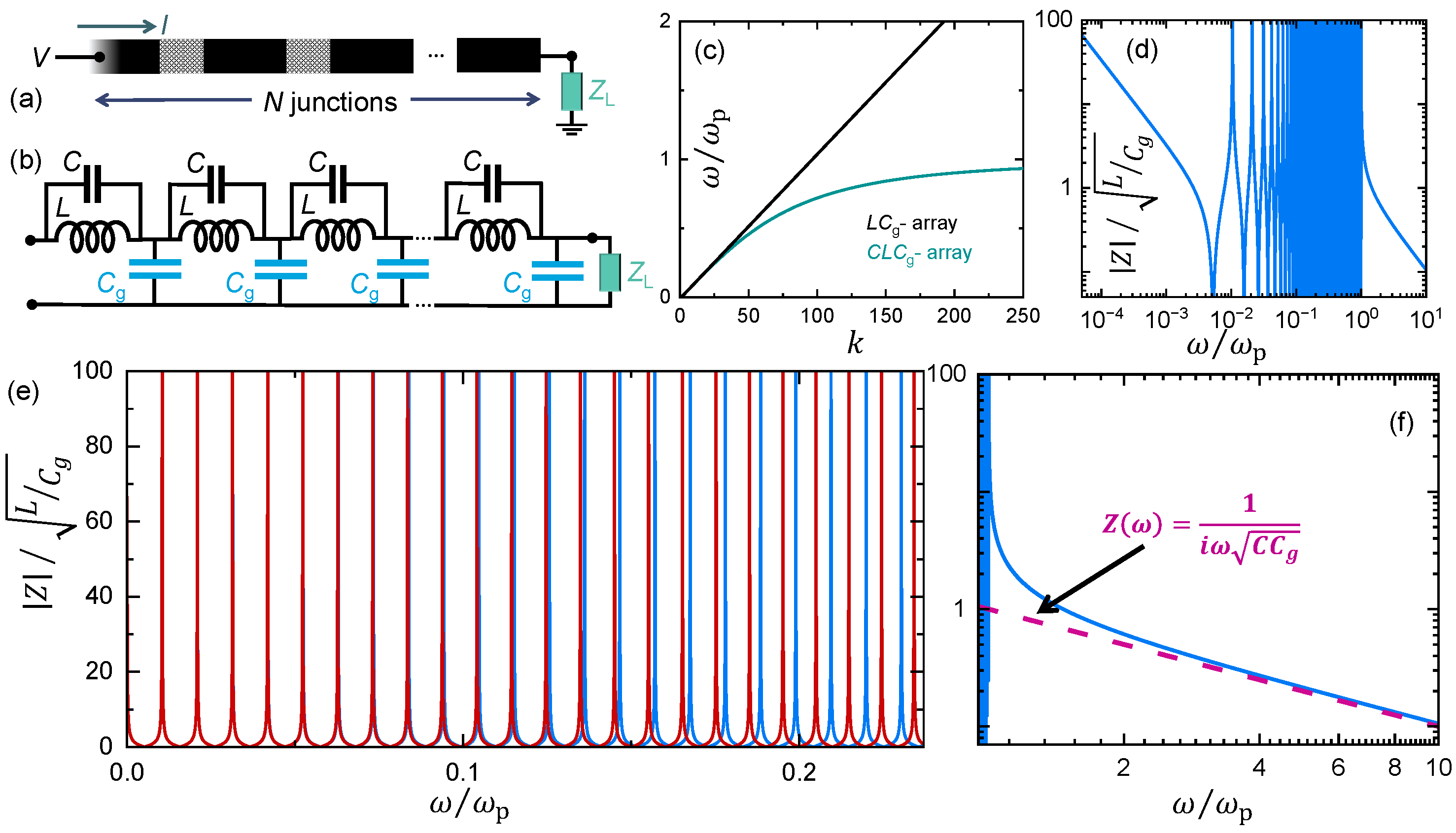
Figure 2.
A qubit coupled to a linear Josephson junction array or a transmission line. (a) A schematic presentation of the circuit. (b) Time-dependent population of the qubit after initialization to the excited state. The transmission line is assumed to be initially in the ground state. The coupling parameter between the qubit and the line is . We have chosen , typically corresponding to either – junctions or a 1 m long transmission line, close to that in Ref. [28]. The value of the impedance has almost no effect on . (c) Initially the qubit decays exponentially, until at the first revival sets abruptly in. The solid line is an exponential fit in this range. The dashed line, also following closely the numerical result, is given by the analytic expression with a decay rate , corresponding to a continuum approximation of frequencies. (d1–d3) Populations of the states in the multimode resonator at three time instants indicated by arrows in (b).

Figure 3.
A qubit coupled to a reservoir of two-level systems in (a). The central qubit is coupled to each TLS via coupling constants that have a uniform distribution between 0 and its maximum level, corresponding to the overall relaxation rate . The dark blue line corresponds to the evolution of in the environment of TLSs with uniform distribution of energies in the range leading to nearly exponential decay. The oscillatory qubit populations of the other curves correspond to uniform environments with for all i, with for grey and red lines, respectively. These dynamics follow that given by Equation (9) quantitatively. (b,c) show the population in a similar distributed bath of and TLSs, respectively, over a time period of . The horizontal lines are the analytical long time predictions given in the text.
Disclaimer/Publisher’s Note: The statements, opinions and data contained in all publications are solely those of the individual author(s) and contributor(s) and not of MDPI and/or the editor(s). MDPI and/or the editor(s) disclaim responsibility for any injury to people or property resulting from any ideas, methods, instructions or products referred to in the content. |
© 2024 by the authors. Licensee MDPI, Basel, Switzerland. This article is an open access article distributed under the terms and conditions of the Creative Commons Attribution (CC BY) license (https://creativecommons.org/licenses/by/4.0/).
Share and Cite
MDPI and ACS Style
Pekola, J.P.; Karimi, B. Heat Bath in a Quantum Circuit. Entropy 2024, 26, 429. https://doi.org/10.3390/e26050429
AMA Style
Pekola JP, Karimi B. Heat Bath in a Quantum Circuit. Entropy. 2024; 26(5):429. https://doi.org/10.3390/e26050429
Chicago/Turabian StylePekola, Jukka P., and Bayan Karimi. 2024. "Heat Bath in a Quantum Circuit" Entropy 26, no. 5: 429. https://doi.org/10.3390/e26050429
Note that from the first issue of 2016, this journal uses article numbers instead of page numbers. See further details here.