Evaluation of Ti–Mn Alloys for Additive Manufacturing Using High-Throughput Experimental Assays and Gaussian Process Regression


Abstract
:1. Introduction
2. Methods
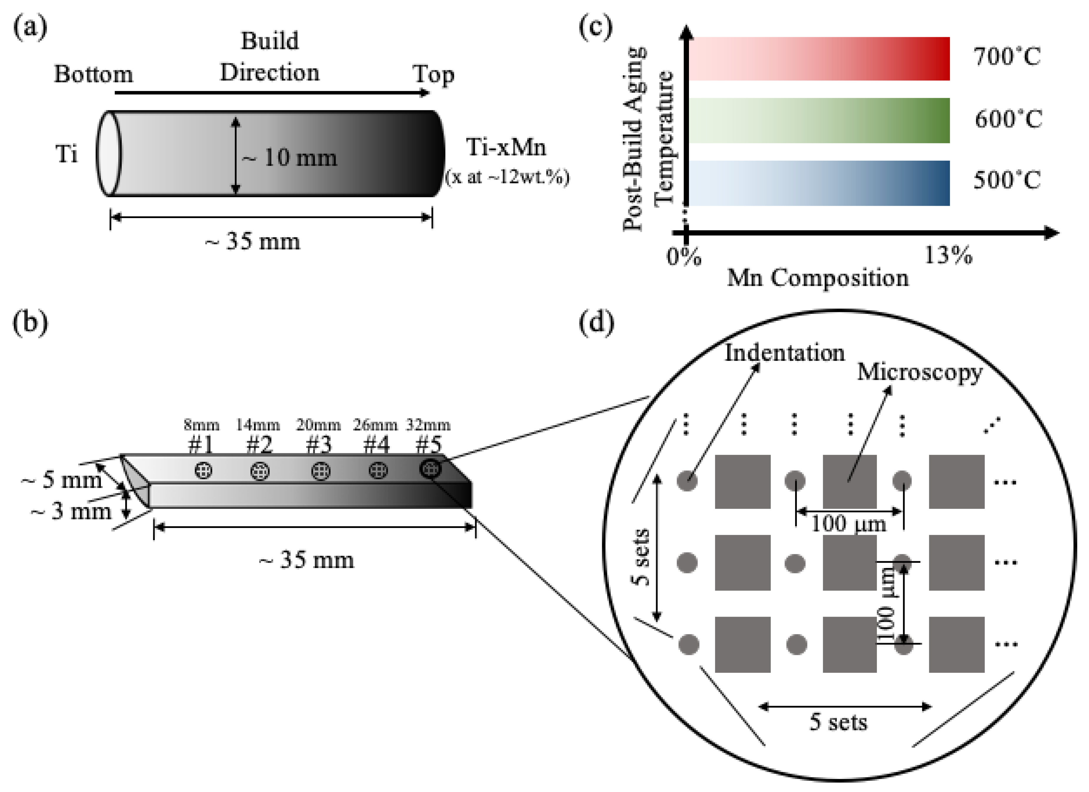
2.1. Experiments
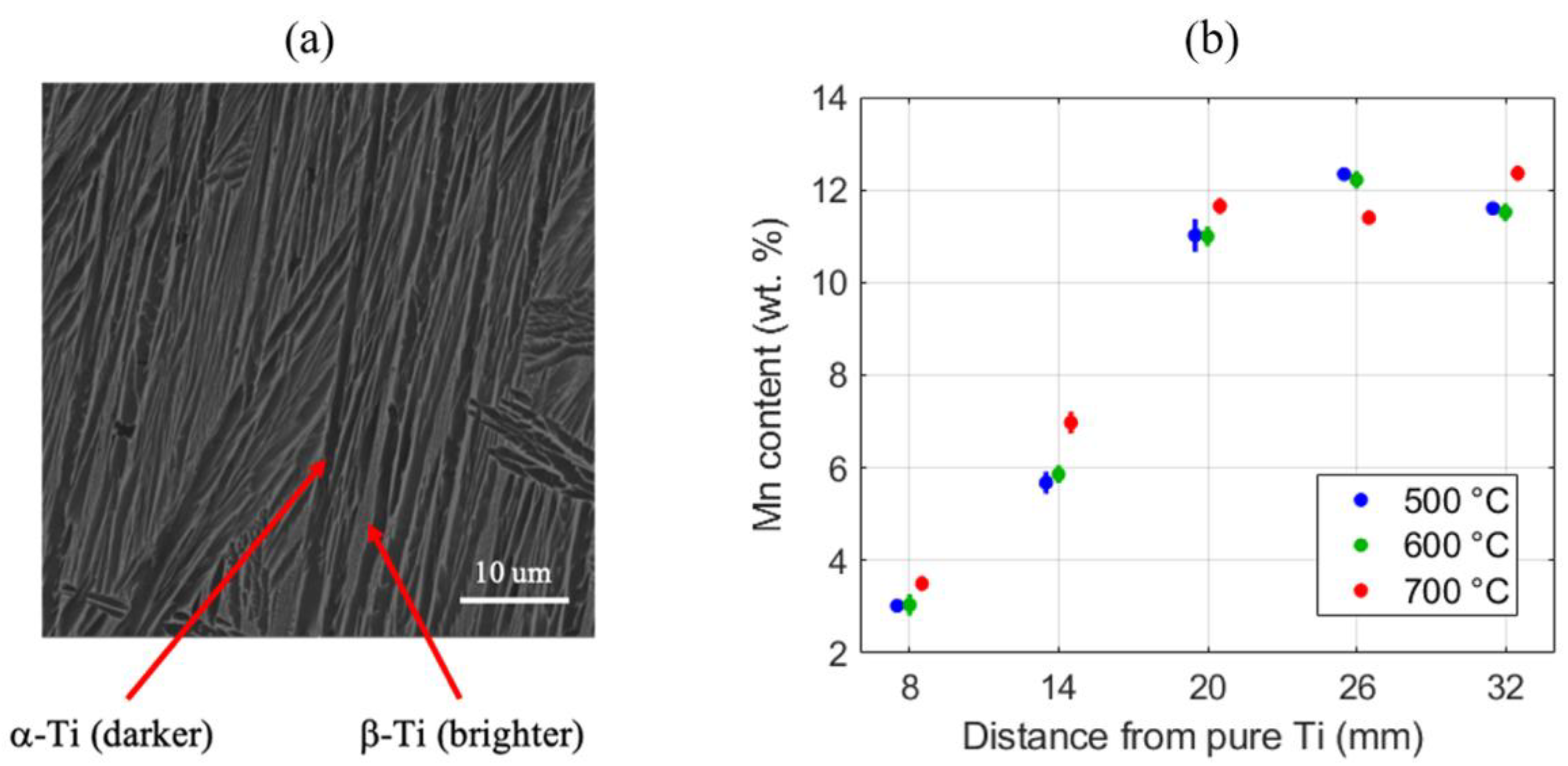
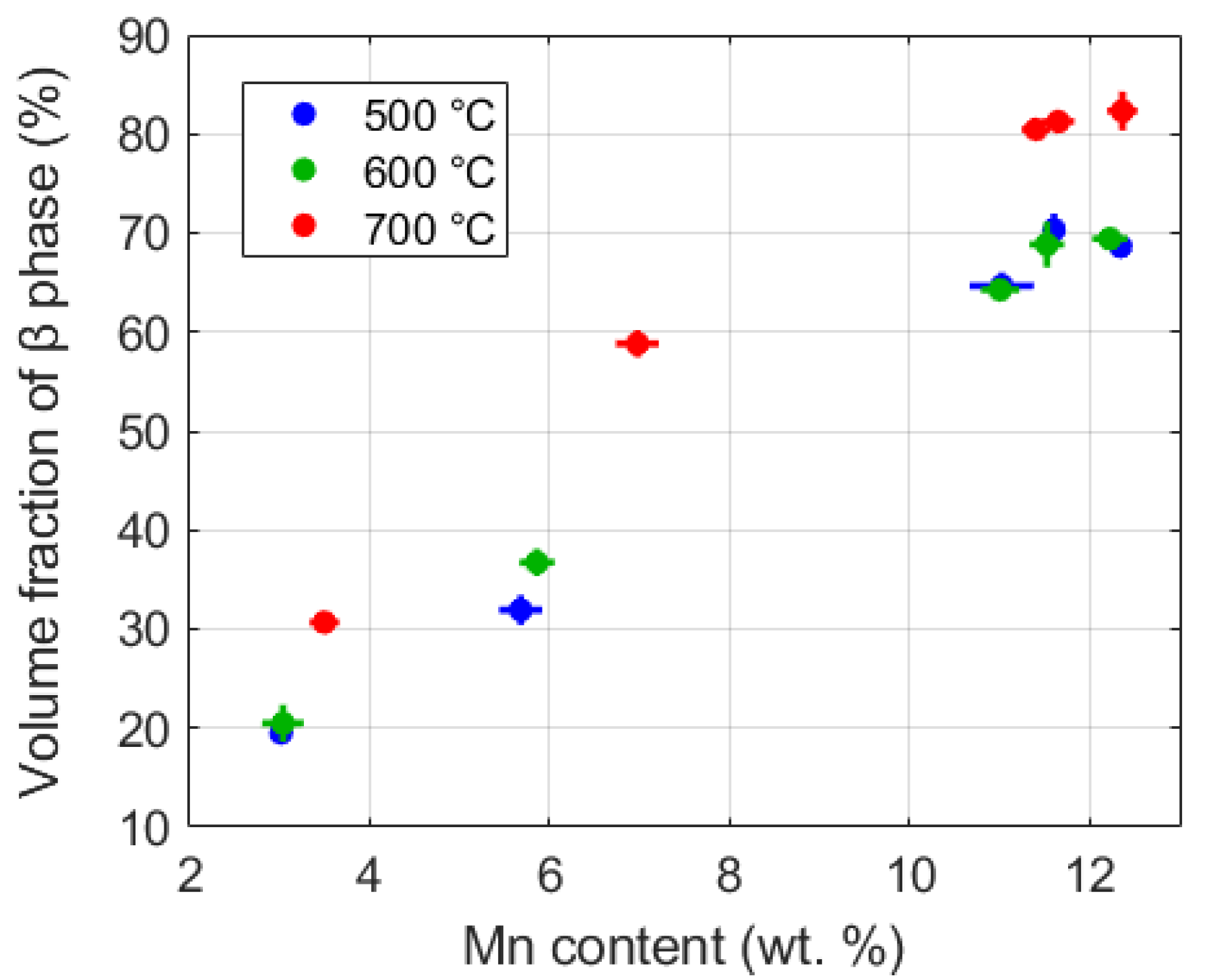
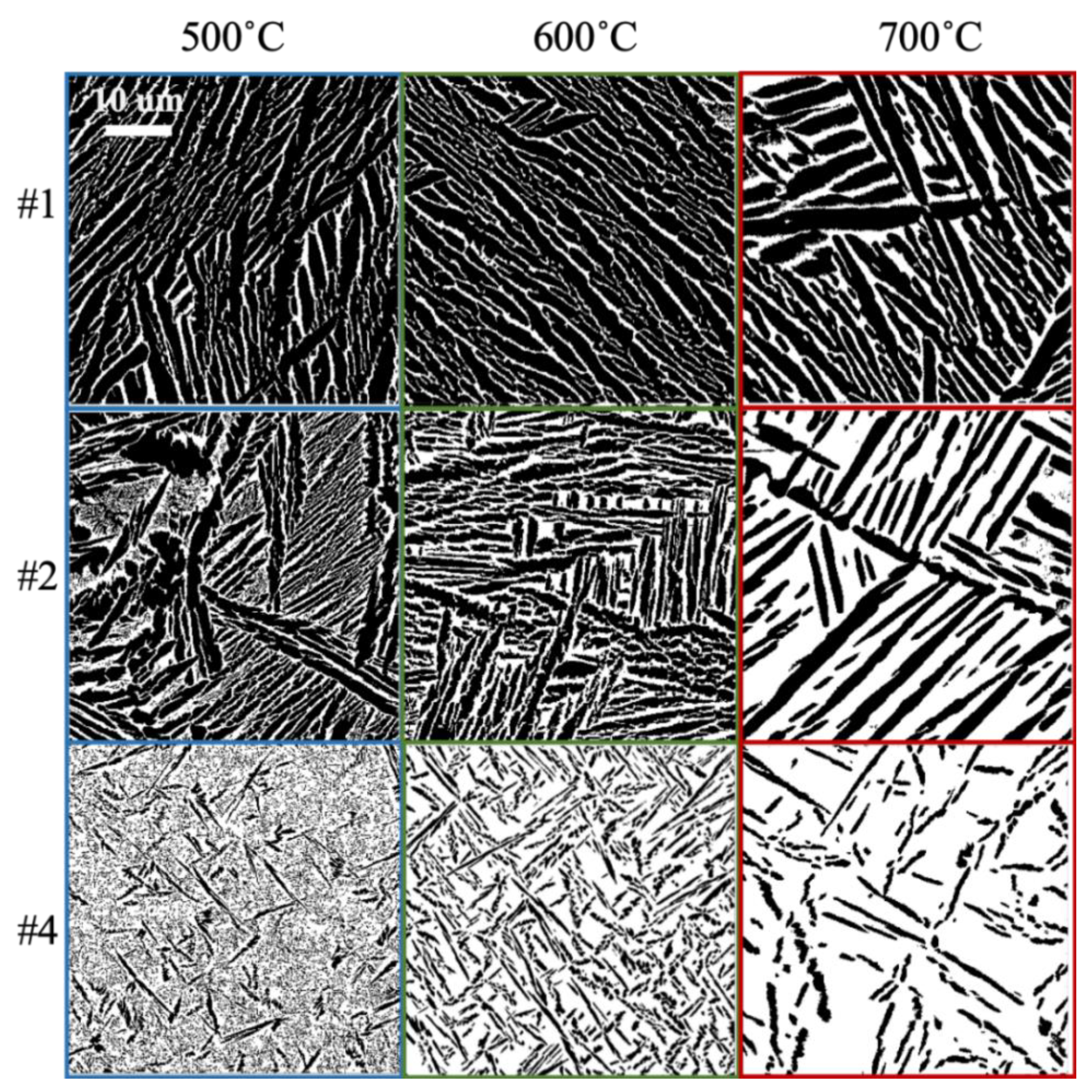
2.2. Microstructure Analysis and Quantification
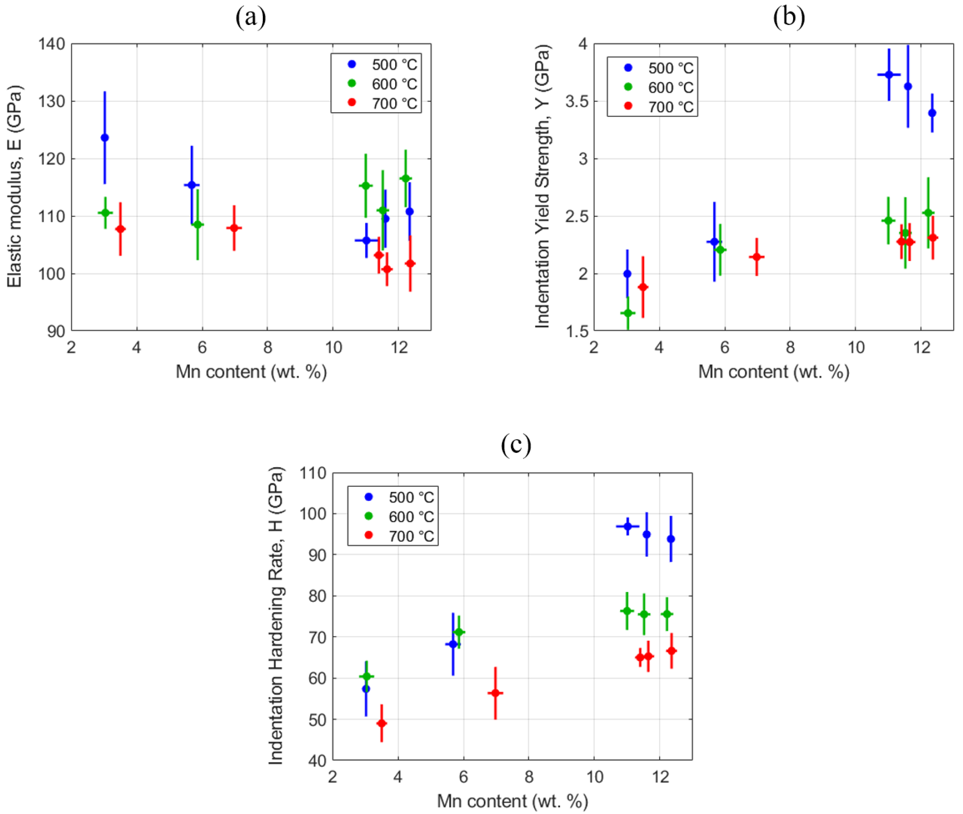
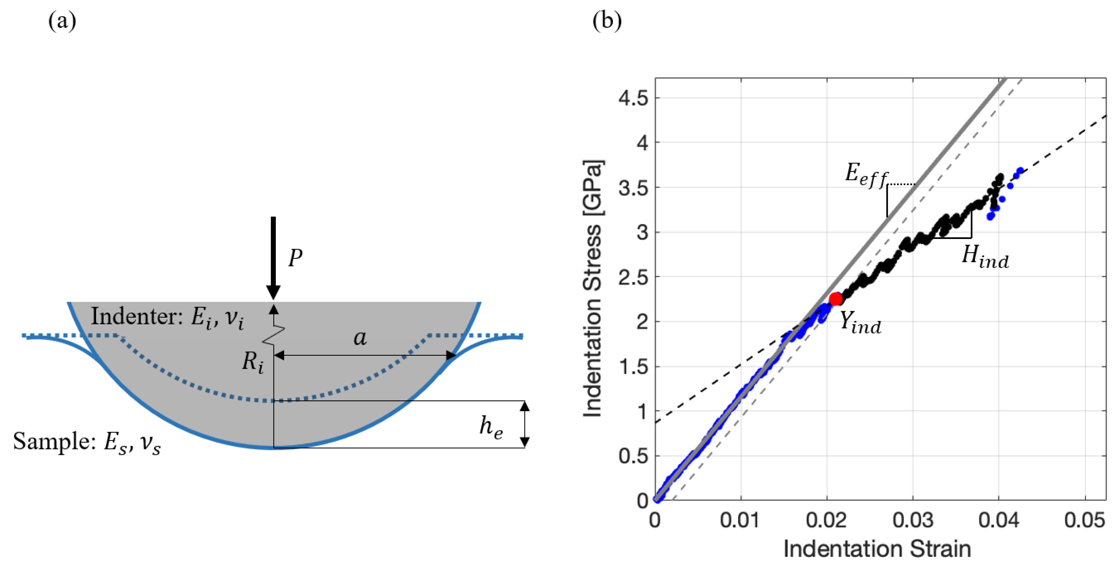
2.3. Mechanical Characterization
2.4. Gaussian Process Modeling
- (1)
- is called the output scaling factor and determines the variance of the output values. A higher value of indicates that the values of the output are widely spread. The ratio of to the output noise (discussed later) determines the uncertainty of the predictions made from the GP model.
- (2)
- and are the interpolation length scale parameters associated with the two input variables and capture the sensitivity of the output variable to the changes in the respective input values. Lower length scale values exhibit shorter memory, leading to sharper fluctuations and more complex nonlinear mapping between the inputs and the output. In other words, lower values of the interpolation length parameter indicate a higher sensitivity of the output to the input value (for the selected input variable). Conversely, larger values of the interpolation length parameters indicate low levels of correlation between the output and the corresponding input variable.
- (3)
- is called the output noise hyperparameter and captures the variance in the training data. For the present study, where the training data are obtained from experiments, this variance can arise from variations in the execution of the experimental assays themselves or variations in the application of the analysis protocols (e.g., image segmentation). is assumed to be the same for the entire input domain (also called homoscedasticity [104]).
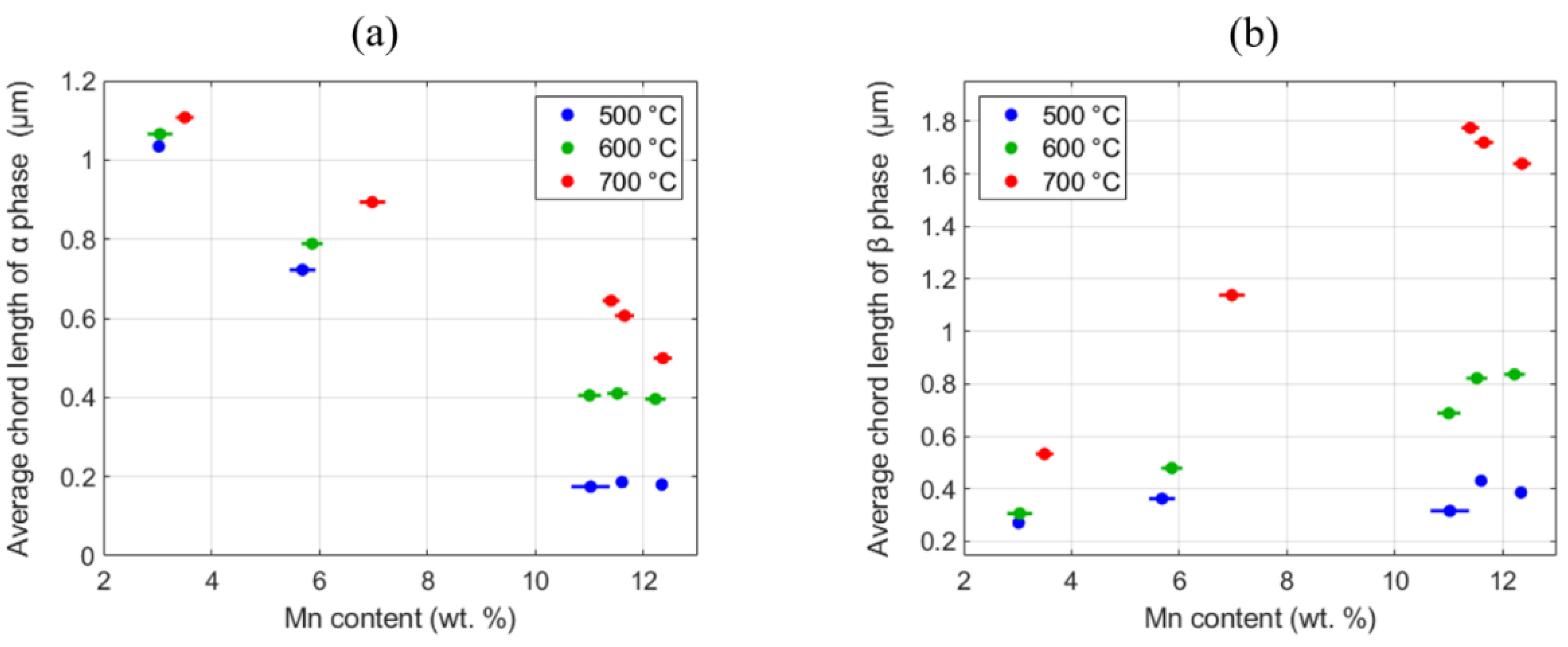
3. Results
4. Discussion
5. Conclusions
Author Contributions
Funding
Conflicts of Interest
References
- Shamsaei, N.; Yadollahi, A.; Bian, L.; Thompson, S.M. An overview of Direct Laser Deposition for additive manufacturing; Part II: Mechanical behavior, process parameter optimization and control. Addit. Manuf. 2015, 8, 12–35. [Google Scholar] [CrossRef]
- Ramirez, D.; Murr, L.; Martinez, E.; Hernandez, D.; Martinez, J.; Machado, B.; Medina, F.; Frigola, P.; Wicker, R. Novel precipitate–microstructural architecture developed in the fabrication of solid copper components by additive manufacturing using electron beam melting. Acta Mater. 2011, 59, 4088–4099. [Google Scholar] [CrossRef]
- Imanian, A.; Leung, K.; Iyyer, N.; Li, P.; Warner, D.H. Optimize Additive Manufacturing Post-Build Heat Treatment and Hot Iso-Static Pressing Process Using an Integrated Computational Materials Engineering Framework. ASME 2018 Int. Mech. Eng. Congr. Expo. 2018, 52019, 00202064. [Google Scholar] [CrossRef]
- Garner, E.; Kolken, H.M.; Wang, C.C.; Zadpoor, A.A.; Wu, J. Compatibility in microstructural optimization for additive manufacturing. Addit. Manuf. 2019, 26, 65–75. [Google Scholar] [CrossRef]
- Wang, Y.; Zhang, L.; Daynes, S.; Zhang, H.; Feih, S.; Wang, M.Y. Design of graded lattice structure with optimized mesostructures for additive manufacturing. Mater. Des. 2018, 142, 114–123. [Google Scholar] [CrossRef]
- Doubrovski, Z.; Verlinden, J.C.; Geraedts, J.M. Optimal design for additive manufacturing: Opportunities and challenges. In Proceedings of the ASME 2011 International Design Engineering Technical Conferences and Computers and Information in Engineering Conference, Washington, DC, USA, 28–31 August 2011; pp. 635–646. [Google Scholar] [CrossRef]
- Gu, D. Laser Additive Manufacturing of High-Performance Materials; Springer: Berlin/Heidelberg, Germany, 2015. [Google Scholar]
- Guo, N.; Leu, M.C. Additive manufacturing: Technology, applications and research needs. Front. Mech. Eng. 2013, 8, 215–243. [Google Scholar] [CrossRef]
- Zhai, Y.; Lados, D.A.; LaGoy, J.L. Additive manufacturing: Making imagination the major limitation. JOM 2014, 66, 808–816. [Google Scholar] [CrossRef] [Green Version]
- Herderick, E. Additive manufacturing of metals: A review. In Proceedings of the Materials Science & Technology Conference and Exhibition 2011 (MS & T 11), Columbus, OH, USA, 16–20 October 2011; pp. 1413–1425. [Google Scholar]
- Vaezi, M.; Chianrabutra, S.; Mellor, B.; Yang, S. Multiple material additive manufacturing–Part 1: A review: This review paper covers a decade of research on multiple material additive manufacturing technologies which can produce complex geometry parts with different materials. Virtual Phys. Prototyp. 2013, 8, 19–50. [Google Scholar] [CrossRef]
- Seepersad, C.C. Challenges and opportunities in design for additive manufacturing. 3D Print. Addit. Manuf. 2014, 1, 10–13. [Google Scholar] [CrossRef]
- Reeves, P.; Tuck, C.; Hague, R. Additive manufacturing for mass customization. In Mass Customization; Springer: London, UK, 2011; pp. 275–289. [Google Scholar] [CrossRef]
- Attaran, M. The rise of 3-D printing: The advantages of additive manufacturing over traditional manufacturing. Bus. Horiz. 2017, 60, 677–688. [Google Scholar] [CrossRef]
- Paoletti, I. Mass customization with additive manufacturing: New perspectives for multi performative building components in architecture. Procedia Eng. 2017, 180, 1150–1159. [Google Scholar] [CrossRef]
- Gu, D.; Ma, C.; Xia, M.; Dai, D.; Shi, Q. A multiscale understanding of the thermodynamic and kinetic mechanisms of laser additive manufacturing. Engineering 2017, 3, 675–684. [Google Scholar] [CrossRef]
- Markl, M.; Körner, C. Multiscale modeling of powder bed–based additive manufacturing. Annu. Rev. Mater. Res. 2016, 46, 93–123. [Google Scholar] [CrossRef]
- Li, C.; Fu, C.; Guo, Y.; Fang, F. A multiscale modeling approach for fast prediction of part distortion in selective laser melting. J. Mater. Process. Technol. 2016, 229, 703–712. [Google Scholar] [CrossRef]
- Francois, M.M.; Sun, A.; King, W.E.; Henson, N.J.; Tourret, D.; Bronkhorst, C.A.; Carlson, N.N.; Newman, C.K.; Haut, T.S.; Bakosi, J. Modeling of additive manufacturing processes for metals: Challenges and opportunities. Curr. Opin. Solid State Mater. Sci. 2017, 21. [Google Scholar] [CrossRef]
- Frazier, W.E. Metal additive manufacturing: A review. J. Mater. Eng. Perform. 2014, 23, 1917–1928. [Google Scholar] [CrossRef]
- Lewandowski, J.J.; Seifi, M. Metal additive manufacturing: A review of mechanical properties. Annu. Rev. Mater. Res. 2016, 46, 151–186. [Google Scholar] [CrossRef] [Green Version]
- Kok, Y.; Tan, X.P.; Wang, P.; Nai, M.; Loh, N.H.; Liu, E.; Tor, S.B. Anisotropy and heterogeneity of microstructure and mechanical properties in metal additive manufacturing: A critical review. Mater. Des. 2018, 139, 565–586. [Google Scholar] [CrossRef]
- Bhavar, V.; Kattire, P.; Patil, V.; Khot, S.; Gujar, K.; Singh, R. A review on powder bed fusion technology of metal additive manufacturing. In Additive Manufacturing Handbook; CRC Press: Boca Raton, FL, USA, 2017; pp. 251–253. [Google Scholar] [CrossRef]
- Ahn, D.-G. Direct metal additive manufacturing processes and their sustainable applications for green technology: A review. Int. J. Precis. Eng. Manuf. Green Technol. 2016, 3, 381–395. [Google Scholar] [CrossRef]
- Gu, G.X.; Chen, C.-T.; Richmond, D.J.; Buehler, M.J. Bioinspired hierarchical composite design using machine learning: Simulation, additive manufacturing, and experiment. Mater. Horiz. 2018, 5, 939–945. [Google Scholar] [CrossRef] [Green Version]
- Reddy, N.; Lee, Y.H.; Park, C.H.; Lee, C.S. Prediction of flow stress in Ti–6Al–4V alloy with an equiaxed α+ β microstructure by artificial neural networks. Mater. Sci. Eng. A 2008, 492, 276–282. [Google Scholar] [CrossRef]
- Lubbers, N.; Lookman, T.; Barros, K. Inferring low-dimensional microstructure representations using convolutional neural networks. Phys. Rev. E 2017, 96, 052111. [Google Scholar] [CrossRef] [Green Version]
- Albuquerque, V.H.C.d.; Alexandria, A.R.d.; Cortez, P.C.; Tavares, J.M.R. Evaluation of multilayer perceptron and self-organizing map neural network topologies applied on microstructure segmentation from metallographic images. NDT E Int. 2009, 42, 644–651. [Google Scholar] [CrossRef]
- Jared, B.H.; Aguilo, M.A.; Beghini, L.L.; Boyce, B.L.; Clark, B.W.; Cook, A.; Kaehr, B.J.; Robbins, J. Additive manufacturing: Toward holistic design. Scr. Mater. 2017, 135, 141–147. [Google Scholar] [CrossRef]
- Haase, C.; Tang, F.; Wilms, M.B.; Weisheit, A.; Hallstedt, B. Combining thermodynamic modeling and 3D printing of elemental powder blends for high-throughput investigation of high-entropy alloys–Towards rapid alloy screening and design. Mater. Sci. Eng. A 2017, 688, 180–189. [Google Scholar] [CrossRef]
- Salzbrenner, B.C.; Rodelas, J.M.; Madison, J.D.; Jared, B.H.; Swiler, L.P.; Shen, Y.-L.; Boyce, B.L. High-throughput stochastic tensile performance of additively manufactured stainless steel. J. Mater. Process. Technol. 2017, 241, 1–12. [Google Scholar] [CrossRef] [Green Version]
- Niendorf, T.; Leuders, S.; Riemer, A.; Brenne, F.; Tröster, T.; Richard, H.A.; Schwarze, D. Functionally graded alloys obtained by additive manufacturing. Adv. Eng. Mater. 2014, 16, 857–861. [Google Scholar] [CrossRef]
- Collins, P.; Banerjee, R.; Banerjee, S.; Fraser, H. Laser deposition of compositionally graded titanium–vanadium and titanium–molybdenum alloys. Mater. Sci. Eng. A 2003, 352, 118–128. [Google Scholar] [CrossRef]
- Banerjee, R.; Collins, P.; Bhattacharyya, D.; Banerjee, S.; Fraser, H. Microstructural evolution in laser deposited compositionally graded α/β titanium-vanadium alloys. Acta Mater. 2003, 51, 3277–3292. [Google Scholar] [CrossRef]
- Banerjee, R.; Bhattacharyya, D.; Collins, P.; Viswanathan, G.; Fraser, H. Precipitation of grain boundary α in a laser deposited compositionally graded Ti–8Al–xV alloy–an orientation microscopy study. Acta Mater. 2004, 52, 377–385. [Google Scholar] [CrossRef]
- Joseph, J.; Jarvis, T.; Wu, X.; Stanford, N.; Hodgson, P.; Fabijanic, D.M. Comparative study of the microstructures and mechanical properties of direct laser fabricated and arc-melted AlxCoCrFeNi high entropy alloys. Mater. Sci. Eng. A 2015, 633, 184–193. [Google Scholar] [CrossRef]
- Gong, X.; Mohan, S.; Mendoza, M.; Gray, A.; Collins, P.; Kalidindi, S. High throughput assays for additively manufactured Ti-Ni alloys based on compositional gradients and spherical indentation. Integr. Mater. Manuf. Innov. 2017, 6, 218–228. [Google Scholar] [CrossRef]
- Khosravani, A.; Cecen, A.; Kalidindi, S.R. Development of high throughput assays for establishing process-structure-property linkages in multiphase polycrystalline metals: Application to dual-phase steels. Acta Mater. 2017, 123, 55–69. [Google Scholar] [CrossRef] [Green Version]
- Weaver, J.S.; Khosravani, A.; Castillo, A.; Kalidindi, S.R. High throughput exploration of process-property linkages in Al-6061 using instrumented spherical microindentation and microstructurally graded samples. Integr. Mater. Manuf. Innov. 2016, 5, 192–211. [Google Scholar] [CrossRef] [Green Version]
- Fernandez-Zelaia, P.; Yabansu, Y.C.; Kalidindi, S.R. A Comparative Study of the Efficacy of Local/Global and Parametric/Nonparametric Machine Learning Methods for Establishing Structure–Property Linkages in High-Contrast 3D Elastic Composites. Integr. Mater. Manuf. Innov. 2019, 8, 67–81. [Google Scholar] [CrossRef]
- Yabansu, Y.C.; Rehn, V.; Hoetzer, J.; Nestler, B.; Kalidindi, S.R. Application of Gaussian process autoregressive models for capturing the time evolution of microstructure statistics from phase-field simulations for sintering of polycrystalline ceramics. Modell. Simul. Mater. Sci. Eng. 2019, 27, 084006. [Google Scholar] [CrossRef]
- Yabansu, Y.C.; Iskakov, A.; Kapustina, A.; Rajagopalan, S.; Kalidindi, S.R. Application of Gaussian process regression models for capturing the evolution of microstructure statistics in aging of nickel-based superalloys. Acta Mater. 2019, 178, 45–58. [Google Scholar] [CrossRef]
- Jung, J.; Yoon, J.I.; Park, H.K.; Kim, J.Y.; Kim, H.S. An efficient machine learning approach to establish structure-property linkages. Comput. Mater. Sci. 2019, 156, 17–25. [Google Scholar] [CrossRef]
- Fernandez-Zelaia, P.; Melkote, S.N. Process-Structure-Property Modeling for Severe Plastic Deformation Processes Using Orientation Imaging Microscopy and Data-Driven Techniques. Integr. Mater. Manuf. Innov. 2019, 8, 17–36. [Google Scholar] [CrossRef]
- Xiong, Y.; Duong, P.L.T.; Wang, D.; Park, S.-I.; Ge, Q.; Raghavan, N.; Rosen, D.W. Data-Driven Design Space Exploration and Exploitation for Design for Additive Manufacturing. J. Mech. Des. 2019, 141, 101101. [Google Scholar] [CrossRef]
- Parvinian, S.; Yabansu, Y.C.; Khosravani, A.; Garmestani, H.; Kalidindi, S.R. High-Throughput Exploration of the Process Space in 18% Ni (350) Maraging Steels via Spherical Indentation Stress–Strain Protocols and Gaussian Process Models. Integr. Mater. Manuf. Innov. 2020, 9. [Google Scholar] [CrossRef]
- Bilionis, I.; Zabaras, N.; Konomi, B.A.; Lin, G. Multi-output separable Gaussian process: Towards an efficient, fully Bayesian paradigm for uncertainty quantification. J. Comput. Phys. 2013, 241, 212–239. [Google Scholar] [CrossRef]
- Hu, Z.; Mahadevan, S. Uncertainty quantification and management in additive manufacturing: Current status, needs, and opportunities. Int. J. Adv. Manuf. Technol. 2017, 93, 2855–2874. [Google Scholar] [CrossRef]
- Chi, G.; Hu, S.; Yang, Y.; Chen, T. Response surface methodology with prediction uncertainty: A multi-objective optimisation approach. Chem. Eng. Res. Des. 2012, 90, 1235–1244. [Google Scholar] [CrossRef]
- Talapatra, A.; Boluki, S.; Duong, T.; Qian, X.; Dougherty, E.; Arróyave, R. Autonomous efficient experiment design for materials discovery with Bayesian model averaging. Phys. Rev. Mater. 2018, 2, 113803. [Google Scholar] [CrossRef]
- Castillo, A.R.; Joseph, V.R.; Kalidindi, S.R. Bayesian Sequential Design of Experiments for Extraction of Single-Crystal Material Properties from Spherical Indentation Measurements on Polycrystalline Samples. JOM 2019, 71, 2671–2679. [Google Scholar] [CrossRef]
- Griffith, M.L.; Harwell, L.D.; Romero, J.T.; Schlienger, E.; Atwood, C.L.; Smugeresky, J.E. Multi-material processing by LENS. In Proceedings of the 1997 International Solid Freeform Fabrication Symposium, Austin, TX, USA, 11–13 August 1997. [Google Scholar]
- Griffith, M.; Keicher, D.; Atwood, C.; Romero, J.; Smugeresky, J.; Harwell, L.; Greene, D. Free form fabrication of metallic components using laser engineered net shaping (LENS). In Proceedings of the 1996 International Solid Freeform Fabrication Symposium, Austin, TX, USA, 12–14 August 1996. [Google Scholar]
- Mudge, R.P.; Wald, N.R. Laser engineered net shaping advances additive manufacturing and repair. Weld. J. 2007, 86, 44. [Google Scholar]
- Avallone, E.A. Marks’ Standard Handbook for Mechanical Engineers; The McGraw-Hill Companies, Inc.: New York, NY, USA, 2007. [Google Scholar]
- Smugeresky, J.; Keicher, D.; Romero, J.; Griffith, M.; Harwell, L. Laser engineered net shaping(LENS) process: Optimization of surface finish and microstructural properties. Adv. Powder Metall. Part Mater. 1997, 3, 21. [Google Scholar] [CrossRef] [Green Version]
- Palčič, I.; Balažic, M.; Milfelner, M.; Buchmeister, B. Potential of laser engineered net shaping (LENS) technology. Mater. Manuf. Process. 2009, 24, 750–753. [Google Scholar] [CrossRef]
- Attar, H.; Ehtemam-Haghighi, S.; Kent, D.; Wu, X.; Dargusch, M.S. Comparative study of commercially pure titanium produced by laser engineered net shaping, selective laser melting and casting processes. Mater. Sci. Eng. A 2017, 705, 385–393. [Google Scholar] [CrossRef]
- Bandyopadhyay, A.; Krishna, B.V.; Xue, W.; Bose, S. Application of laser engineered net shaping (LENS) to manufacture porous and functionally graded structures for load bearing implants. J. Mater. Sci. Mater. Med. 2009, 20, 29. [Google Scholar] [CrossRef] [PubMed]
- Jeon, T.; Hwang, T.; Yun, H.; VanTyne, C.; Moon, Y. Control of Porosity in Parts Produced by a Direct Laser Melting Process. Appl. Sci. 2018, 8, 2573. [Google Scholar] [CrossRef] [Green Version]
- Wang, L.; Pratt, P.; Felicelli, S.D.; Kadiri, H.E.; Berry, J.T.; Wang, P.T.; Horstemeyer, M.F. Experimental analysis of porosity formation in laser-assisted powder deposition process. Miner. Met. Mater. Soc. 2009, 1, 389–396. [Google Scholar]
- Li, L. Repair of directionally solidified superalloy GTD-111 by laser-engineered net shaping. J. Mater. Sci. 2006, 41, 7886–7893. [Google Scholar] [CrossRef]
- Korinko, P.; Adams, T.; Malene, S.; Gill, D.; Smugeresky, J. Laser Engineered Net Shaping® for Repair and Hydrogen Compatibility. Weld. J. 2011, 90, 171–181. [Google Scholar]
- Liu, Z.; Cong, W.; Kim, H.; Ning, F.; Jiang, Q.; Li, T.; Zhang, H.-C.; Zhou, Y. Feasibility Exploration of Superalloys for AISI 4140 Steel Repairing using Laser Engineered Net Shaping. Procedia Manuf. 2017, 10, 912–922. [Google Scholar] [CrossRef]
- Wilson, J.M.; Piya, C.; Shin, Y.C.; Zhao, F.; Ramani, K. Remanufacturing of turbine blades by laser direct deposition with its energy and environmental impact analysis. J. Clean. Prod. 2014, 80, 170–178. [Google Scholar] [CrossRef]
- Liu, D.; Lippold, J.C.; Li, J.; Rohklin, S.R.; Vollbrecht, J.; Grylls, R. Laser engineered net shape (LENS) technology for the repair of Ni-base superalloy turbine components. Metall. Mater. Trans. A 2014, 45, 4454–4469. [Google Scholar] [CrossRef]
- Balla, V.K.; Bandyopadhyay, P.P.; Bose, S.; Bandyopadhyay, A. Compositionally graded yttria-stabilized zirconia coating on stainless steel using laser engineered net shaping (LENS™). Scr. Mater. 2007, 57, 861–864. [Google Scholar] [CrossRef]
- Balla, V.K.; DeVasConCellos, P.D.; Xue, W.; Bose, S.; Bandyopadhyay, A. Fabrication of compositionally and structurally graded Ti–TiO2 structures using laser engineered net shaping (LENS). Acta Biomater. 2009, 5, 1831–1837. [Google Scholar] [CrossRef]
- Polanski, M.; Kwiatkowska, M.; Kunce, I.; Bystrzycki, J. Combinatorial synthesis of alloy libraries with a progressive composition gradient using laser engineered net shaping (LENS): Hydrogen storage alloys. Int. J. Hydrogen Energy 2013, 38, 12159–12171. [Google Scholar] [CrossRef]
- Bandyopadhyay, P.P.; Balla, V.K.; Bose, S.; Bandyopadhyay, A. Compositionally graded aluminum oxide coatings on stainless steel using laser processing. J. Am. Ceram. Soc. 2007, 90, 1989–1991. [Google Scholar] [CrossRef]
- Zhang, Y.; Bandyopadhyay, A. Direct fabrication of compositionally graded Ti-Al2O3 multi-material structures using Laser Engineered Net Shaping. Addit. Manuf. 2018, 21, 104–111. [Google Scholar] [CrossRef]
- Hofmann, D.C.; Roberts, S.; Otis, R.; Kolodziejska, J.; Dillon, R.P.; Suh, J.-O.; Shapiro, A.A.; Liu, Z.-K.; Borgonia, J.-P. Developing gradient metal alloys through radial deposition additive manufacturing. Sci. Rep. 2014, 4, 5357. [Google Scholar] [CrossRef]
- Lütjering, G.; Williams, J.C. Titanium; Springer-Science & Business Media: Berlin/Heidelberg, Germany, 2007. [Google Scholar]
- Bobet, J.L.; Darriet, B. Relationship between hydrogen sorption properties and crystallography for TiMn2 based alloys. Int. J. Hydrog. Energy 2000, 25, 767–772. [Google Scholar] [CrossRef]
- Zhang, F.; Weidmann, A.; Nebe, J.B.; Beck, U.; Burkel, E. Preparation, microstructures, mechanical properties, and cytocompatibility of TiMn alloys for biomedical applications. J. Biomed. Mater. Res. Part B Appl. Biomater. 2010, 94B, 406–413. [Google Scholar] [CrossRef]
- Takada, Y.; Nakajima, H.; Okuno, O.; Okabe, T. Microstructure and Corrosion Behavior of Binary Titanium Alloys with Beta-stabilizing Elements. Dent. Mater. J. 2001, 20, 34–52. [Google Scholar] [CrossRef] [PubMed]
- Murray, J.L. The Mn-Ti (Manganese-Titanium) system. Bull. Alloy Phase Diagr. 1981, 2, 334–343. [Google Scholar] [CrossRef]
- Mitchell, A.; Kawakami, A.; Cockcroft, S. Beta fleck and segregation in titanium alloy ingots. High Temp. Mater. Process. 2006, 25, 337–349. [Google Scholar] [CrossRef]
- Seagle, S.; Yu, K.; Giangiordano, S. Considerations in processing titanium. Mater. Sci. Eng. A 1999, 263, 237–242. [Google Scholar] [CrossRef]
- Bomberger, H.; Froes, F. The melting of titanium. JOM 1984, 36, 39–47. [Google Scholar] [CrossRef]
- Gammon, L.M.; Briggs, R.D.; Packard, J.M.; Batson, K.W.; Boyer, R.; Domby, C.W. Metallography and microstructures of titanium and its alloys. ASM Handb. 2004, 9, 899–917. [Google Scholar] [CrossRef]
- Weaver, J.S.; Priddy, M.W.; McDowell, D.L.; Kalidindi, S.R. On capturing the grain-scale elastic and plastic anisotropy of alpha-Ti with spherical nanoindentation and electron back-scattered diffraction. Acta Mater. 2016, 117, 23–34. [Google Scholar] [CrossRef] [Green Version]
- Vachhani, S.J.; Doherty, R.D.; Kalidindi, S.R. Effect of the continuous stiffness measurement on the mechanical properties extracted using spherical nanoindentation. Acta Mater. 2013, 61, 3744–3751. [Google Scholar] [CrossRef]
- Otsu, N. A threshold selection method from gray-level histograms. IEEE Trans. Syst. Man Cybern. Part A 1979, 9, 62–66. [Google Scholar] [CrossRef] [Green Version]
- Sezgin, M.; Sankur, B. Survey over image thresholding techniques and quantitative performance evaluation. J. Electron. Imaging 2004, 13, 146–166. [Google Scholar] [CrossRef]
- Siddique, M.A.B.; Arif, R.B.; Khan, M.M.R. Digital Image Segmentation in Matlab: A Brief Study on OTSU’s Image Thresholding. In Proceedings of the 2018 International Conference on Innovation in Engineering and Technology (ICIET), Dhaka, Bangladesh, 27–28 December 2018; pp. 1–5. [Google Scholar] [CrossRef]
- Turner, D.M.; Niezgoda, S.R.; Kalidindi, S.R. Efficient computation of the angularly resolved chord length distributions and lineal path functions in large microstructure datasets. Modell. Simul. Mater. Sci. Eng. 2016, 24, 075002. [Google Scholar] [CrossRef] [Green Version]
- Torquato, S. Random Heterogeneous Materials: Microstructure and Macroscopic Properties; Springer Science & Business Media: New York, NY, USA, 2013; Volume 16. [Google Scholar]
- Latypov, M.I.; Kühbach, M.; Beyerlein, I.J.; Stinville, J.-C.; Toth, L.S.; Pollock, T.M.; Kalidindi, S.R. Application of chord length distributions and principal component analysis for quantification and representation of diverse polycrystalline microstructures. Mater. Charact. 2018, 145, 671–685. [Google Scholar] [CrossRef]
- Pathak, S.; Stojakovic, D.; Doherty, R.; Kalidindi, S.R. Importance of surface preparation on the nano-indentation stress-strain curves measured in metals. J. Mater. Res. 2009, 24, 1142–1155. [Google Scholar] [CrossRef]
- Pathak, S.; Kalidindi, S.R. Spherical nanoindentation stress–strain curves. Mater. Sci. Eng. R Rep. 2015, 91, 1–36. [Google Scholar] [CrossRef] [Green Version]
- Kalidindi, S.R.; Pathak, S. Determination of the effective zero-point and the extraction of spherical nanoindentation stress–strain curves. Acta Mater. 2008, 56, 3523–3532. [Google Scholar] [CrossRef]
- Hertz, H.; Jones, D.E.; Schott, G.A. Miscellaneous Papers; Macmillan and Company: London, UK, 1896. [Google Scholar]
- Johnson, K.L.; Johnson, K.L. Contact Mechanics; Cambridge University Press: Cambridge, UK, 1987. [Google Scholar]
- Oliver, W.C.; Pharr, G.M. An improved technique for determining hardness and elastic modulus using load and displacement sensing indentation experiments. J. Mater. Res. 1992, 7, 1564–1583. [Google Scholar] [CrossRef]
- Li, X.; Bhushan, B. A review of nanoindentation continuous stiffness measurement technique and its applications. Mater. Charact. 2002, 48, 11–36. [Google Scholar] [CrossRef]
- Pathak, S.; Kalidindi, S.R.; Mara, N.A. Investigations of orientation and length scale effects on micromechanical responses in polycrystalline zirconium using spherical nanoindentation. Scr. Mater. 2016, 113, 241–245. [Google Scholar] [CrossRef] [Green Version]
- Pathak, S.; Stojakovic, D.; Kalidindi, S.R. Measurement of the local mechanical properties in polycrystalline samples using spherical nanoindentation and orientation imaging microscopy. Acta Mater. 2009, 57, 3020–3028. [Google Scholar] [CrossRef]
- Patel, D.K.; Al-Harbi, H.F.; Kalidindi, S.R. Extracting single-crystal elastic constants from polycrystalline samples using spherical nanoindentation and orientation measurements. Acta Mater. 2014, 79, 108–116. [Google Scholar] [CrossRef]
- Williams, C.K.; Rasmussen, C.E. Gaussian Processes for Machine Learning; MIT Press: Cambridge, MA, USA, 2006; Volume 2. [Google Scholar]
- Bishop, C.M. Pattern Recognition and Machine Learning (Information Science and Statistics); Springer: Berlin/Heidelberg, Germany, 2006. [Google Scholar]
- Yabansu, Y.C.; Altschuh, P.; Hötzer, J.; Selzer, M.; Nestler, B.; Kalidindi, S.R. A digital workflow for learning the reduced-order structure-property linkages for permeability of porous membranes. Acta Mater. 2020, 195, 668–680. [Google Scholar] [CrossRef]
- Witte, R.S.; Witte, J.S. Statistics; Wiley: Hoboken, NJ, USA, 2009. [Google Scholar]
- Dette, H.; Munk, A. Testing heteroscedasticity in nonparametric regression. J. R. Stat. Soc. Ser. B Stat. Methodol. 1998, 60, 693–708. [Google Scholar] [CrossRef]
- Weaver, J.S.; Kalidindi, S.R. Mechanical characterization of Ti-6Al-4V titanium alloy at multiple length scales using spherical indentation stress-strain measurements. Mater. Des. 2016, 111, 463–472. [Google Scholar] [CrossRef] [Green Version]
- Mohammed, M.T.; Khan, Z.A.; Siddiquee, A.N. Beta titanium alloys: The lowest elastic modulus for biomedical applications: A review. Int. J. Chem. Mol. Nucl. Mater. Metall. Eng. 2014, 8, 726–731. [Google Scholar] [CrossRef]
- Laheurte, P.; Prima, F.; Eberhardt, A.; Gloriant, T.; Wary, M.; Patoor, E. Mechanical properties of low modulus β titanium alloys designed from the electronic approach. J. Mech. Behav. Biomed. Mater. 2010, 3, 565–573. [Google Scholar] [CrossRef] [PubMed]
- Santos, P.F.; Niinomi, M.; Liu, H.; Cho, K.; Nakai, M.; Itoh, Y.; Narushima, T.; Ikeda, M. Fabrication of low-cost beta-type Ti–Mn alloys for biomedical applications by metal injection molding process and their mechanical properties. J. Mech. Behav. Biomed. Mater. 2016, 59, 497–507. [Google Scholar] [CrossRef] [PubMed]
- Welsch, G.; Boyer, R.; Collings, E. Materials Properties Handbook: Titanium Alloys; ASM International: Materials Park, OH, USA, 1993. [Google Scholar]
- Patel, D.K.; Kalidindi, S.R. Correlation of spherical nanoindentation stress-strain curves to simple compression stress-strain curves for elastic-plastic isotropic materials using finite element models. Acta Mater. 2016, 112, 295–302. [Google Scholar] [CrossRef] [Green Version]
- Cho, K.; Niinomi, M.; Nakai, M.; Liu, H.; Santos, P.F.; Itoh, Y.; Ikeda, M.; Narushima, T. Improvement in mechanical strength of low-cost β-type Ti–Mn alloys fabricated by metal injection molding through cold rolling. J. Alloys Compd. 2016, 664, 272–283. [Google Scholar] [CrossRef]
- Alshammari, Y.; Yang, F.; Bolzoni, L. Mechanical properties and microstructure of Ti-Mn alloys produced via powder metallurgy for biomedical applications. J. Mech. Behav. Biomed. Mater. 2019, 91, 391–397. [Google Scholar] [CrossRef]
- Santos, P.F.; Niinomi, M.; Cho, K.; Nakai, M.; Liu, H.; Ohtsu, N.; Hirano, M.; Ikeda, M.; Narushima, T. Microstructures, mechanical properties and cytotoxicity of low cost beta Ti–Mn alloys for biomedical applications. Acta Biomater. 2015, 26, 366–376. [Google Scholar] [CrossRef]


| GPR Results | CL α | CL β | VF-β | Y | H | E |
|---|---|---|---|---|---|---|
| 667.17 | 141.85 | 263.23 | 199.12 | 143.38 | 211.78 | |
| 10.95 | 10.48 | 9.39 | 16.83 | 14.78 | 12.49 | |
| 19.52 | 18.47 | 0.55 | 2.48 | 53.97 | 92.17 | |
| 0.93 | 1.66 | 0.01 | 0.17 | 2.64 | 1.39 | |
| 20.88 | 11.13 | 45.59 | 14.50 | 20.41 | 66.10 | |
| MAPE | 6.89 | 9.87 | 3.54 | 6.26 | 3.32 | 2.02 |
Publisher’s Note: MDPI stays neutral with regard to jurisdictional claims in published maps and institutional affiliations. |
© 2020 by the authors. Licensee MDPI, Basel, Switzerland. This article is an open access article distributed under the terms and conditions of the Creative Commons Attribution (CC BY) license (http://creativecommons.org/licenses/by/4.0/).
Share and Cite
Gong, X.; Yabansu, Y.C.; Collins, P.C.; Kalidindi, S.R. Evaluation of Ti–Mn Alloys for Additive Manufacturing Using High-Throughput Experimental Assays and Gaussian Process Regression. Materials 2020, 13, 4641. https://doi.org/10.3390/ma13204641
Gong X, Yabansu YC, Collins PC, Kalidindi SR. Evaluation of Ti–Mn Alloys for Additive Manufacturing Using High-Throughput Experimental Assays and Gaussian Process Regression. Materials. 2020; 13(20):4641. https://doi.org/10.3390/ma13204641
Chicago/Turabian StyleGong, Xinyi, Yuksel C. Yabansu, Peter C. Collins, and Surya R. Kalidindi. 2020. "Evaluation of Ti–Mn Alloys for Additive Manufacturing Using High-Throughput Experimental Assays and Gaussian Process Regression" Materials 13, no. 20: 4641. https://doi.org/10.3390/ma13204641