1. Introduction
In Iowa, the dominant contributor to streamflow is the runoff generated from regional watersheds, which are characterized by more natural terrain, but the urban areas primarily experience the negative effects of fluvial and pluvial flooding [
1,
2]. Hydrological and hydraulic models are commonly used as tools to understand past, present, and future flood risk profiles at various scales. [
1,
3,
4,
5]. Integrating regional- and local-scale hydrological models is difficult because of the varying heterogenous spatial and temporal scales and dimensionality within the watershed [
6,
7,
8]. These kinds of challenges are not unique to Iowa.
In this study, the authors simulated historical peak streamflow and urban flood extents using a nested regional–local model with three radar rainfall products as inputs. In the context of this paper, “nested” refers to one-way coupling of a coarse resolution model to a model with a finer resolution. We use “local” to refer to an urban area of interest that is within a “regional” watershed where rural landscapes and natural terrain are dominant. We used a nested model to study flooding in a small town, Manchester, IA in the regional Maquoketa River basin (
Figure 1). This area was suitable for a case study because we were able to use radar rainfall products, streamflow measurements, rain gauge data, and the statewide forecasting model managed by the Iowa Flood Center (IFC). Our objective was to gain an improved understanding of the impacts of the spatial and temporal resolution of radar rainfall at the regional and local scales for extreme rainfall events, and to identify the benefits of using a nested modeling approach for streamflow prediction and local flood modeling.
A hydrological and hydraulic model developed at the regional scale is typically used to generate streamflow estimates along a major stream network, and the dominant rainfall–runoff and routing processes can be described at a coarser scale (i.e., datasets at a resolution of 50 m or greater) and with simplifications (such as channel geometry) [
1,
9,
10,
11]. Local hydrodynamic models are developed on an “as needed” basis for a specific purpose, with a desired set of output variables and accuracy such as floodplain mapping or evaluating changes in the water level from a proposed engineering project [
12,
13]. In these cases, a fine-resolution model is often necessary for simulating pluvial flooding in an urban landscape, because the dominant hydrologic processes vary spatially and temporally due to increasingly complex drainage networks with subsurface (e.g., storm sewers) and surface (e.g., streets, buildings) routing. To get an accurate depiction of water movement through urban morphologies, hydrological models should account for these flow interchanges and the resulting impact on water surface elevations. [
14,
15,
16]. By using a nested modeling approach, we were able to one-way couple a coarse-resolution model, suitable for characterizing regional rainfall–runoff, to a fine-resolution model required for local flood information [
17,
18].
An important source of uncertainty in hydrological models is the spatiotemporal resolution of the rainfall input (see Villarini and Krajewski [
19] for a review of radar rainfall uncertainty modeling), because it heavily influences the rainfall–runoff processes simulated in the model [
20,
21,
22]. Many researchers seek to accurately capture the non-linear, spatiotemporal patterns of rainfall and how this variability will change the accuracy of flood models and their predictions [
20,
22,
23,
24,
25,
26,
27,
28]. Furthermore, radar and satellite rainfall datasets can be resolved and used as input to local scale or urban models [
20,
22,
25,
27,
29]. By using multiple rainfall inputs, we produced an ensemble of hydrological predictions that implicitly accounted for the uncertainty in the equations and parameters that were used to describe the physical system [
30]. In this paper, the authors describe the study area and historical flood events, the data and modeling framework, and the model’s performance when predicting streamflow and urban flood extents. Lastly, we discuss some general observations and conclusions drawn from this study that will inform modelers on the benefits and limitations of using a nested regional–local model and multiple radar rainfall inputs for predicting streamflow.
2. Study Area
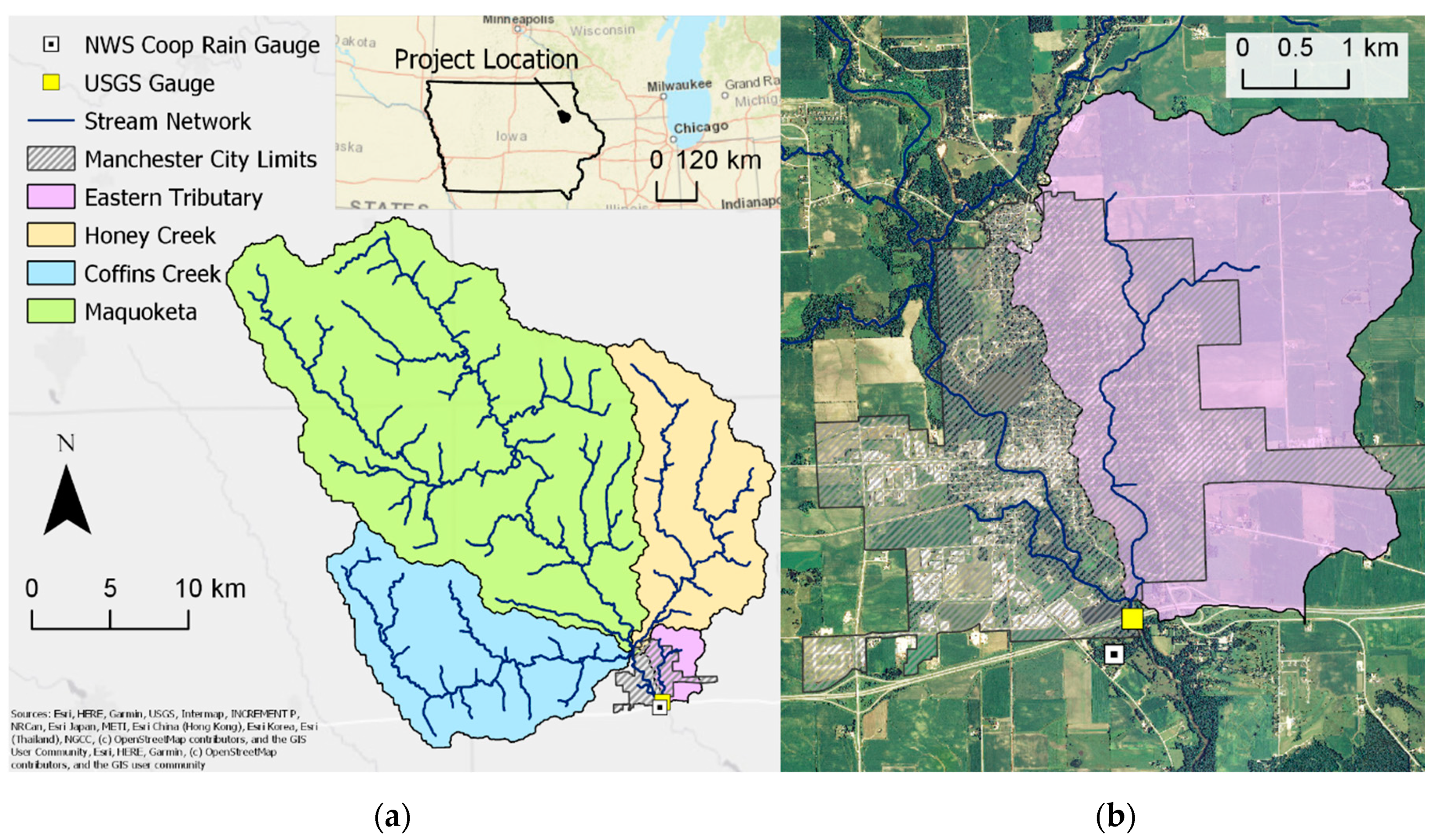
The city of Manchester covers an area of approximately 12.2 km
2 and is located along the Maquoketa River in the northeastern region of Iowa (
Figure 1). The watershed upstream of Manchester is 712 km
2 of agricultural land, and the eastern bank of the Maquoketa River draining through Manchester is approximately 15 m lower than the west bank, which is adjacent to downtown. The city experienced costly flooding nine times between 2002 and 2017 when the river exceeded the National Weather Service (NWS) Moderate Flood Stage of 5.2 m. In addition to riverine flooding, the eastern neighborhoods experience nuisance flooding after an extreme storm occurs locally, overwhelming the drainage network. The risk increases when local flooding occurs coincident with a high tailwater level in the Maquoketa River.
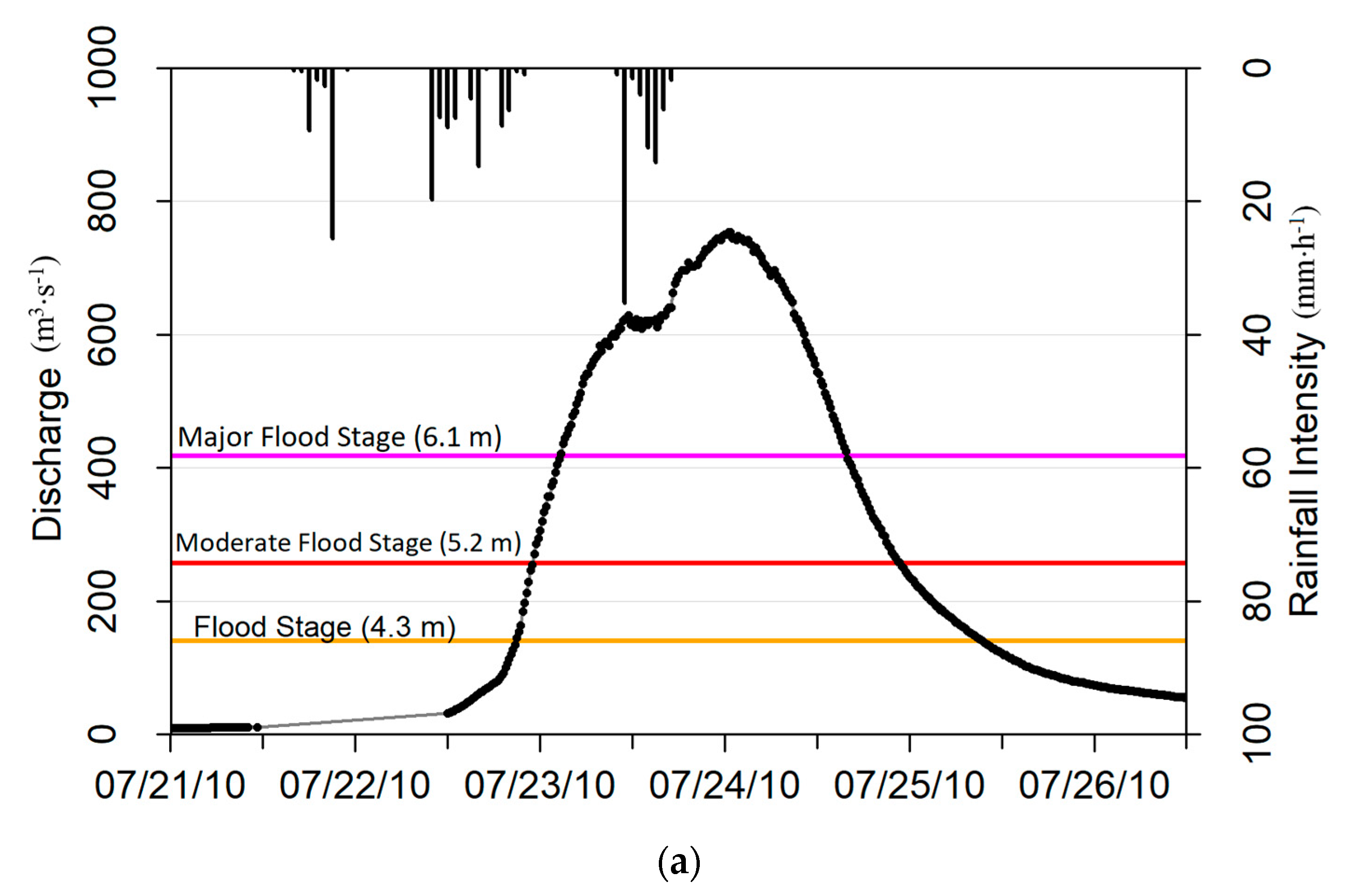
One of the more memorable fluvial flooding events occurred after a regional extreme storm passed over northeast Iowa in July 2010, resulting in the highest recorded stage of 7.5 m on the Maquoketa River at Manchester (
Figure 2a). The July 2010 flood had an annual flood probability range of 0.2–1%, which is a recurrence interval of 500 to 100 years. The flood waters remained above the NWS “major flood” stage for over 37 h, resulting in over
$850,000 of recorded project costs in Delaware County [
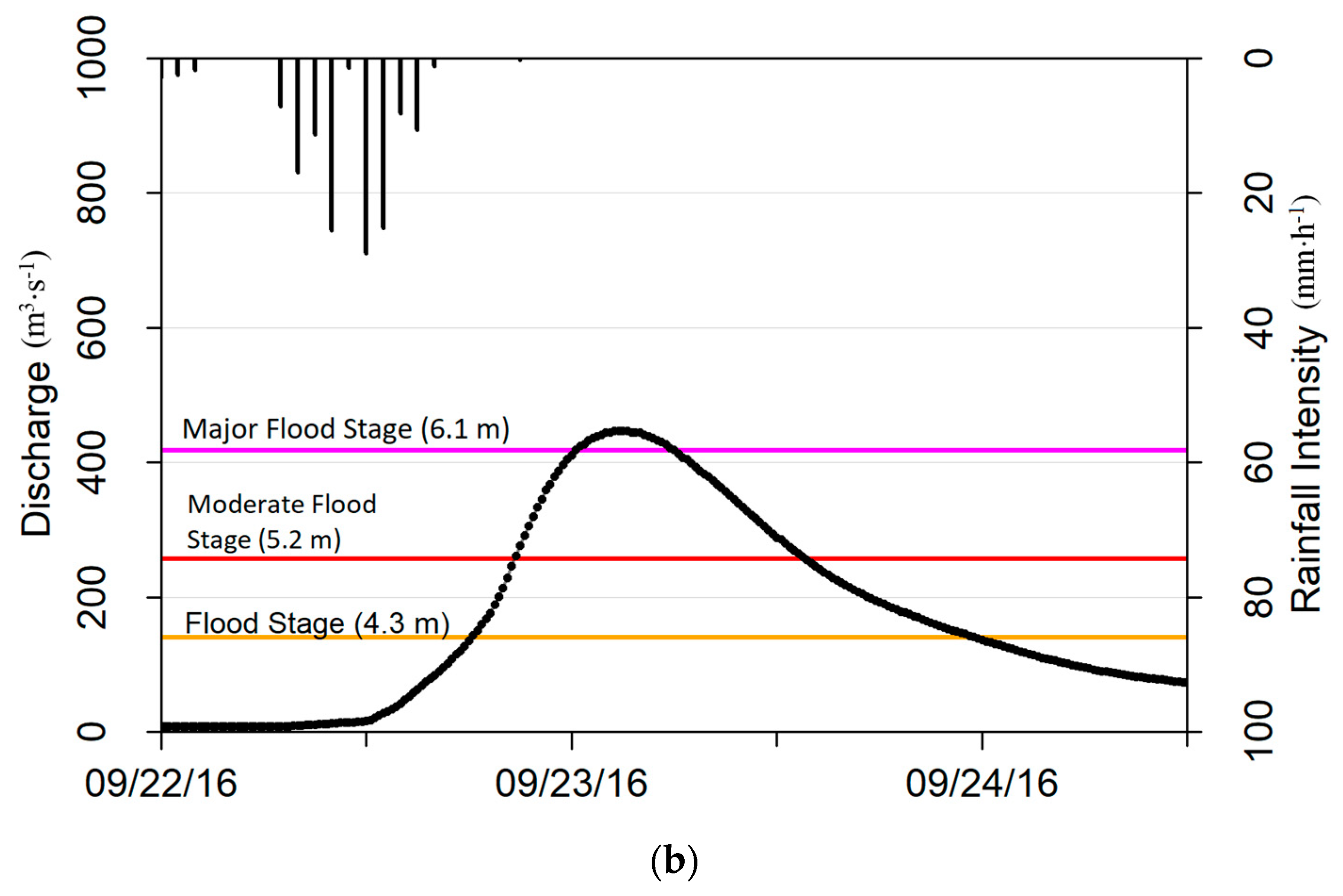
31]. In September 2016, the local area experienced high rainfall intensities over a short period of time in the lower portion of the basin (
Figure 2b). Local officials recall this event because of the quick hydrological response of the watershed compared to previous historical floods.
3. Data and Methods
We developed a simulation framework to investigate how the scale of hydrological models and the resolution of their inputs, specifically rainfall, can improve streamflow predictions with a nested modeling approach. We modeled the local area in XPSWMM, which is a one-dimensional and two-dimensional (1D/2D) spatially distributed model used for simulating hydrological and hydraulic processes [
32]. In the regional area, we used the hillslope-link model (HLM), which is a distributed model developed at the IFC to be robust, requiring significantly less computer effort than hydrodynamic models because it has lower demands on the representation and accuracy of the flow dynamics [
1]. The two physics-based models used in this study differ in their approach to hydrological modeling, but, by using a nested modeling approach, we were able to investigate how coupling these models built with different scales (i.e., regional and local) could add value to our understanding of streamflow predictions in watersheds with urban and rural landscapes. Additional information on the models and the data used is provided in the following sections. For both the local and the regional model, we used a calibration-free approach, i.e., a common configuration of parameters determined a priori applied for all the model inputs, and no adjustments were made for specific basins [
1]. We considered that calibrating would obscure our understanding of the hydrological system, and that model calibration compensates for the errors in the model inputs and modeling processes.
3.1. Regional Model
The regional area was modeled using the HLM, a distributed model that decomposes the landscape into hillslopes and channels. The HLM solves the mass conservation equations within the four hillslope layers and between the channels and hillslopes using ordinary differential equations. The portion of rainfall that becomes runoff is determined by the near-surface soil saturation and the hydraulic soil properties. The complex drainage and landcover patterns in urban areas are not necessarily captured by the HLM’s simplified infiltration process at the land surface. To route flow through the river network, HLM uses a power law wherein the water velocity is related to the discharge and upstream drainage area. HLM does consider the variability of flow across the stream network, but it does not account for reservoirs or include local hydraulic considerations. It considers variability of flow in the different channels of the network, but it does not include local hydraulic considerations or backwater effects from reservoirs. Additional information on the HLM can be found in References [
5] and [
33]. The performance of the HLM has been extensively evaluated using seven years of radar rainfall data. Model simulations of streamflow have been compared to observed values at approximately 140 USGS streamflow gauges in Iowa, showing skillful performance, especially for eastern Iowa basins [
4].
3.2. Local Model
The urban area was modeled in XPSWMM, where we used area-average radar rainfall estimates as inputs. We derived land use, soil type, and other hydrological parameters from national datasets, but did not use calibration to correct the local model’s behavior. With an unclear understanding of the soil and landcover in the area, there was a risk of over-calibrating the model to fit the solution. For this study, we did not calibrate because we considered the average (or typical) values to be suitable for accurately modeling the runoff and flow paths in the local model.
Soil data were retrieved from the National Soil Survey Geographic (SSURGO) database and we determined that the prominent soil types in the local model consisted of loam and sand [
34]. We modeled losses due to infiltration using the Green–Ampt equation [
32]. The soil types and parameters, specifically saturated hydraulic conductivities, covered a wide range of values because soils are redistributed and compacted at varying levels throughout the watershed [
35]. The infiltration parameters are often difficult to estimate without in situ measurements, so the average values used in the local model were derived from the typical values listed in References [
32] and [
36]. We derived the land surface properties from geospatial datasets, including impervious cover and land use from high-resolution landcover for Delaware County in 2009 [
37]. The Manning’s n values (roughness) vary significantly in space and are difficult to estimate, particularly in floodplains [
38], so we used the typical range of roughness values for the different land types as specified by the Natural Resources Conservation Service [
39]. Representing buildings in a hydrodynamic model can be done by manipulating the terrain to include them in the topography or by imposing an additional head loss to the model grid [
40,
41,
42,
43,
44]. We modeled the buildings as a landcover type with varying vertical roughness to account for storage.
We manually digitized the layout of the subsurface and surface drainage network and the corresponding hydraulic parameters (i.e., geometry, elevation data, and conveyance information) using engineering drawings, surveys, and local knowledge. We incorporated multiple sets of river cross-sectional data and routing information directly into XPSWMM from models built using the Hydrologic Engineering Center River Analysis System (HEC-RAS) by the U.S. Army Corps of Engineers (USACE) and the Iowa Department of Natural Resources (IDNR). The final XPSWMM model had 862 nodes that represented common features in the storm-sewer network, including outfalls, culverts, intakes, and manholes. The nodes were connected with over 20.1 km of links that represented the storm sewers in the network (see
Figure 3b). We modeled the storm sewers as pipe flow, the natural channels as open channel flow, and bridge and inline structures were modeled in 1D. The 1D drainage network was connected to the 2D domain at nodes (intakes and outfalls) and polyline interfaces (the river or channel banks). Hydrodynamic models are commonly used for urban flood modeling [
45,
46,
47], where the minimum grid resolution is determined by the width of the streets or the size of the buildings [
48,
49]. We used a 1.5 m digital terrain model (DTM) derived from 1 m LiDAR topography from the 2007–2010 Iowa LiDAR Project [
37] to extract terrain information that was used by grids applied in XPSWMM. The 2D domain was 7.5 km
2 and we used a 4.6 and 9.1 m (15 and 30 ft) grid-cell size to balance accuracy and computational efficiency.
3.3. Simulation Framework
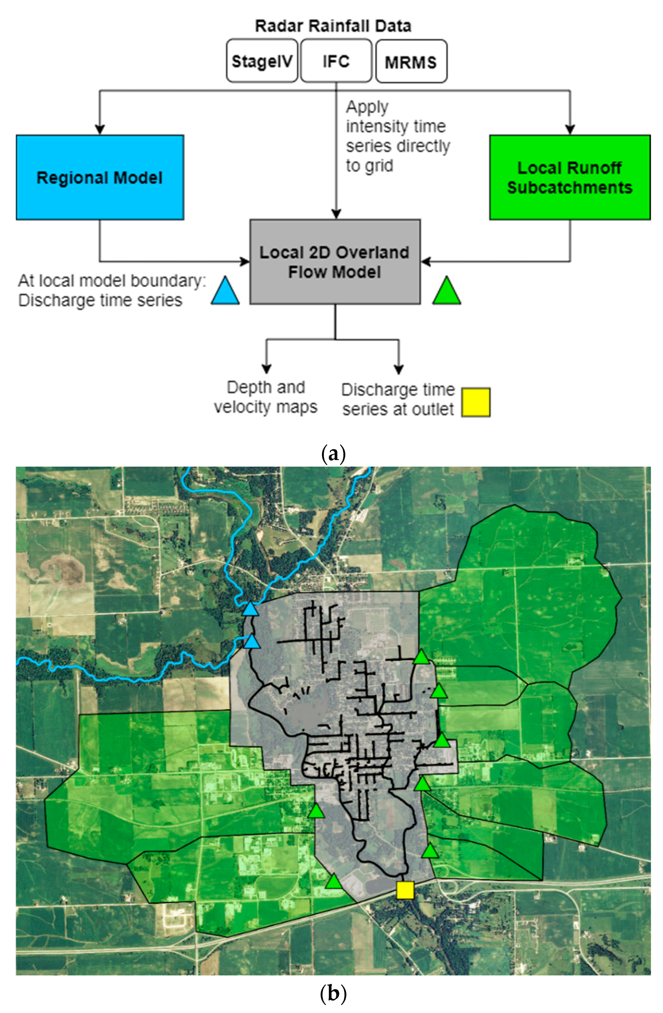
We set up the simulation framework to compare the impacts of radar rainfall spatiotemporal resolution on streamflow predictions generated by the regional model and the nested regional–local model. A schematic of the framework is shown in
Figure 3a. We applied three radar rainfall products to both the regional and local models, including
Multi-radar multi-sensor (MRMS) rainfall estimates which were rain-gauge-bias corrected, with temporal resolution of 1 h and a spatial resolution of 1 km [
50];
Stage IV rainfall estimates which were rain-gauge-bias corrected with a temporal resolution of 1 h and a spatial resolution of 4 km [
51]; and
IFC rainfall estimates that did not include rain-gauge-bias correction, with a temporal resolution of 1 h and 5 min and a spatial resolution of 500 m [
52,
53,
54].
The radar rainfall estimates were compared to rainfall observations and daily accumulation records available from the NWS Coop rain gauge located just outside the city limits (Station ID: MHRI4) [
55] (see
Figure 1).
For the regional model, we generated initial conditions in the watershed using a spin-up period that started a minimum of three months before the selected events. In the local model, we set the initial soil moisture conditions to be partially dry with the simulation starting at least six hours before the onset of rain, which allowed time for the natural channels to fill from regional streamflow inputs. We set the initial state of the storm sewers and drainage network components to be empty. First, we generated regional runoff using the HLM model and used the streamflow outputs at various locations as the inflow boundary conditions to the XPSWMM model. The boundary conditions applied to the XPSWMM model included (1) spatially averaged radar rainfall estimates directly applied to the 2D domain and (2) the pre—simulated HLM streamflow as inflow boundary conditions to the stream network (
Figure 3). The results of the one-way-coupled, nested-model simulations were compared to the HLM model simulations and both were evaluated against measured USGS streamflow of the Maquoketa River (05416900-USGS, MCHI4-NWS) located downstream of the city. The results are referred to herein by the model configuration and the rainfall input used (IFC, Stage IV hourly and 5 min, and MRMS), where HLM refers to the regional model and XP—C2 is the nested regional–local model.
4. Results and Evaluation
The model output was validated against two flood events (July 2010 and September 2016) during which the Maquoketa River stage exceeded the NWS major flood stage, resulting in nuisance flooding in Manchester. For both events, we compared the spatial pattern of the radar rainfall estimates over the region to each other. We also compared radar rainfall totals that occurred locally to a nearby NWS Coop rain gauge that had daily measurements. The primary method of validation we used was a statistical analysis to compare simulated streamflow to measured USGS observations. We used the most up-to-date rating curve to calculate the stage from the simulated discharge at the models (HLM and XP—C2) outlet. We used the root-mean-square error (RMSE) to quantify the difference between the modeled stage and the observed stage. To quantify the forecast error in the time series, we used the mean absolute error (MAE) and the coefficient of determination (R2) [
56], and to measure the model’s ability to reproduce the magnitude and timing of the peak flows we used the peak error (PE) and the time to peak error (TPE) [
56,
57,
58,
59]. We considered the magnitude and timing of the peak and the rising and receding limb of the hydrograph when determining the suitability of the model to predict streamflow. Additionally, the model’s ability to capture the time to crest and the duration above the NWS major flood stage (6.1 m) was important for Manchester, because these statistics indicate significant flooding downtown. We considered the model’s performance suitable for streamflow predictions if it was able to predict the flood stage within 0.6–0.9 m of the rising limb, which is typically the error for issued flood warnings across Iowa [
60]. In addition to streamflow statistics, we used a visual qualitative comparison to examine the urban model’s (i.e., XPSWMM) ability to generally reproduce the flood extent and depths for the two extreme rainfall events. We used non-georeferenced photos and drone footage to validate the performance of the local model to predict the flow of water in the urban environment.
4.1. Radar Rainfall Estimates
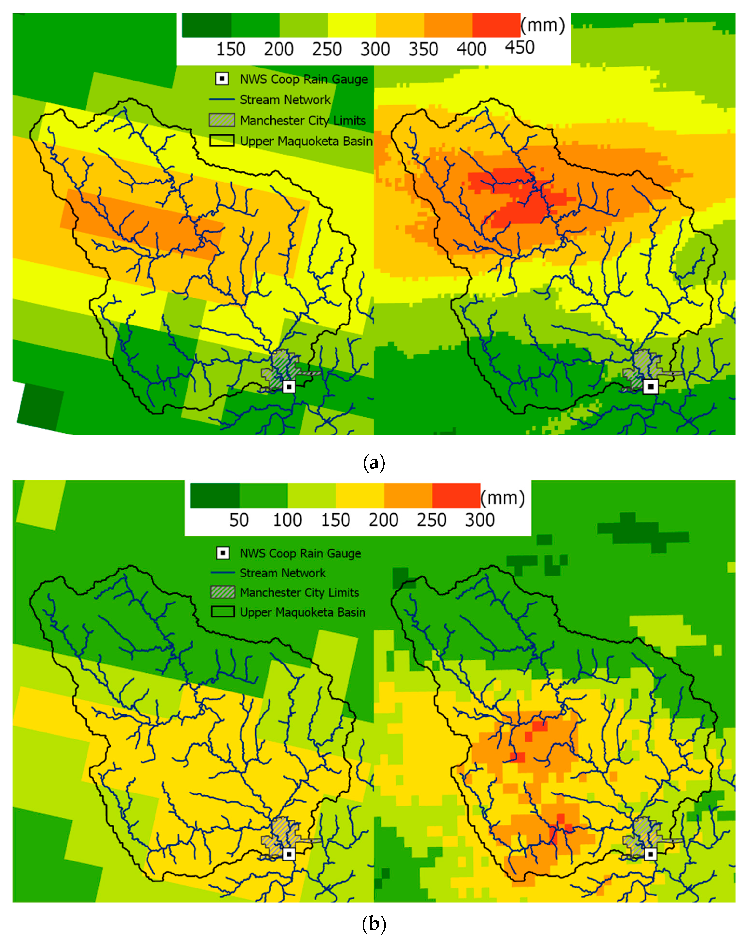
During July 2010, the upper Maquoketa River basin and Manchester received 406 mm and 203 mm of rainfall, respectively (
Figure 4a). More recently, in September 2016, over 152 mm of rainfall occurred over Manchester in 17 h, while nearly 178 mm dropped over the upper Maquoketa River basin (
Figure 4b).
Note that for the September 2016 storm, the radar rainfall estimates (MRMS and Stage IV) showed similar spatial patterns and any differences in total accumulation are a result of the different methods used to create each rainfall product. The rainfall products with a finer spatial resolution (IFC and MRMS) showed a variation in the distribution of the rainfall across the basins, but in general, the pattern and total rainfall was similar to Stage IV. The study area had limited rainfall-gauge data, so the quality control check was limited for the radar rainfall products. The radar rainfall grids across all three products were considered equally uncertain and, given the lack of rain-gauge data in the area, we did not reconstruct or adjust the precipitation grids. As shown in
Table 1, the radar rainfall products were used to compute the accumulated precipitation and maximum rainfall intensity of the storm over Manchester city limits. These measurements gave us information on the total rainfall but not the spatial distribution of the radar rainfall. We calculated the difference between the radar rainfall estimates and the NWS Coop rain gauge daily measurements. The accumulated radar rainfall estimates were greater than the daily records measured at the NWS Coop rain gauge by 5–9% for Stage IV and MRMS and by 16–21% for IFC.
4.2. Modeled Streamflow
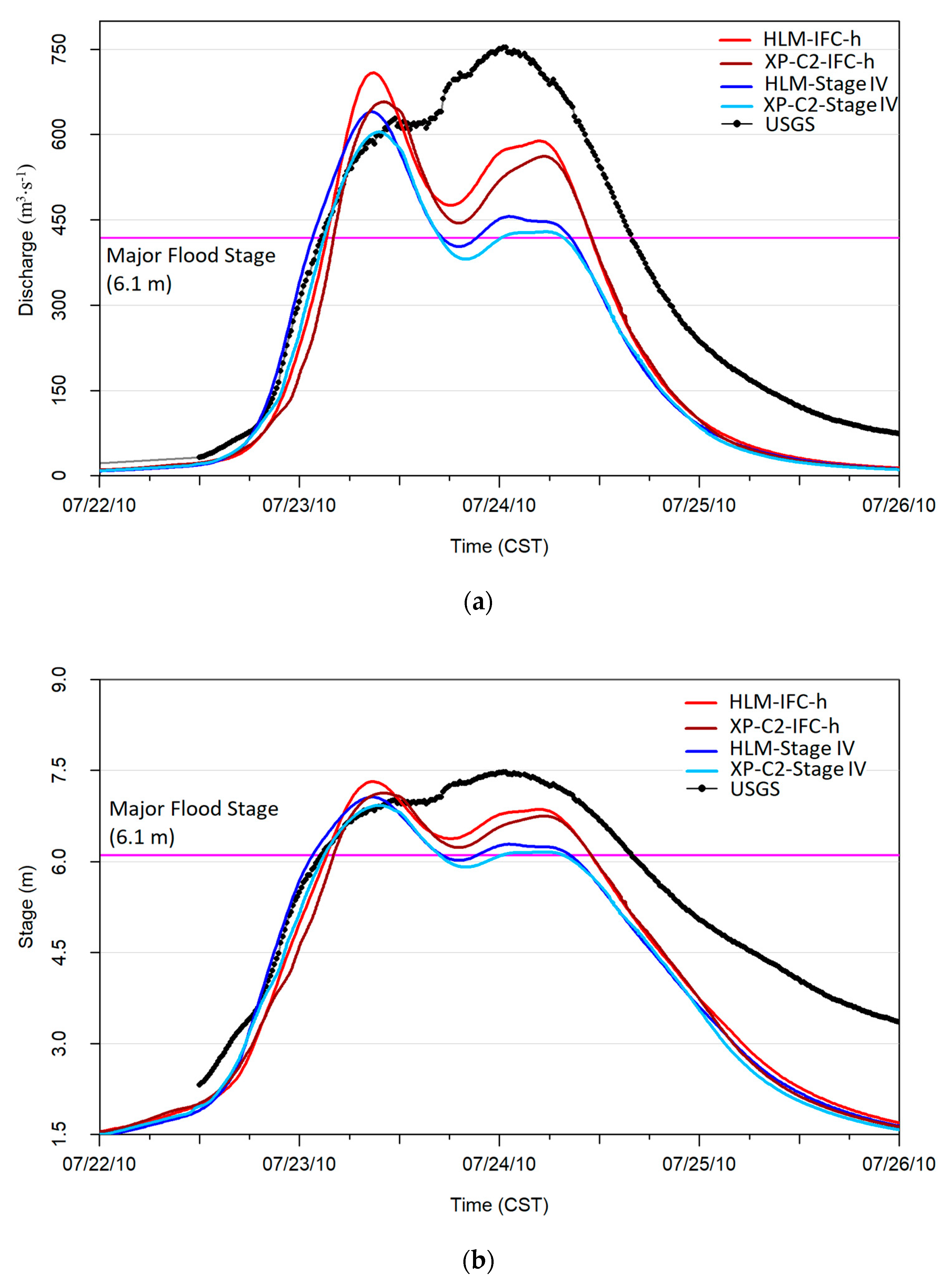
For the storm event of July 2010, the simulated hydrographs shown in
Figure 5a illustrate the skill of both the regional (HLM) and nested (XP—C2) models when predicting the rising limb of the hydrograph and the first peak. We also noticed that the nested model consistently generated a lower discharge compared to the regional model, which is discussed later. Both the nested and the regional models predicted the initial crest of the major flood stage earlier than what was observed, and also underestimated the rising limb by 0.3–0.5 m (
Figure 5b). After the first peak, the observed flood stage continued to increase, but the models showed a recession of the flood waters. The overall shape of the simulated hydrographs using both Stage IV and IFC radar rainfall estimates indicated that the models generated runoff from the rainfall occurring after the first peak, but there was a significant volume of water unaccounted for. The spatial and temporal variability of rainfall–runoff over the regional area was investigated, but no significant discrepancies in model routing and rainfall distribution were evident. The missing volume in the hydrograph may have been an issue of the total rainfall–runoff from the regional model and a discrepancy in the routing of high water levels in the floodplain where water is attenuated and stored. We noted that there might be downstream infrastructure creating backwater effects that were not represented in the local or regional model. One example is the breach of the Delhi Dam on 24 July 2010, located 17.7 km downstream of Manchester. The designed storage volume of the dam was 12,000 km
3 and the breach released over 1960 m
3⋅s
−1, but it is unlikely to have resulted in a significant backwater effect that would account for the missing volume in the hydrograph [
61].
We computed statistics for the first and second peaks of the hydrograph separately. We obtained root-mean-squared error (RMSE), mean absolute error (MAE), coefficient of determination (R2), peak error (PE), time to peak error (TPE), time to major flood stage error, and duration above major flood stage. The results are shown in
Table 2. We saw that both the nested and regional model had skill in reproducing the magnitude of the first peak with a PE of less than 0.3 m, but the error doubled when predicting the magnitude of the second peak. The ensemble of hydrological predictions could be used by city officials to predict the time at which the Maquoketa River will crest 6.1 m, giving them time to prepare. The recession was not included in this analysis because our main interest was in the model’s ability to capture the rising limb, peak, and duration above the flood stage.
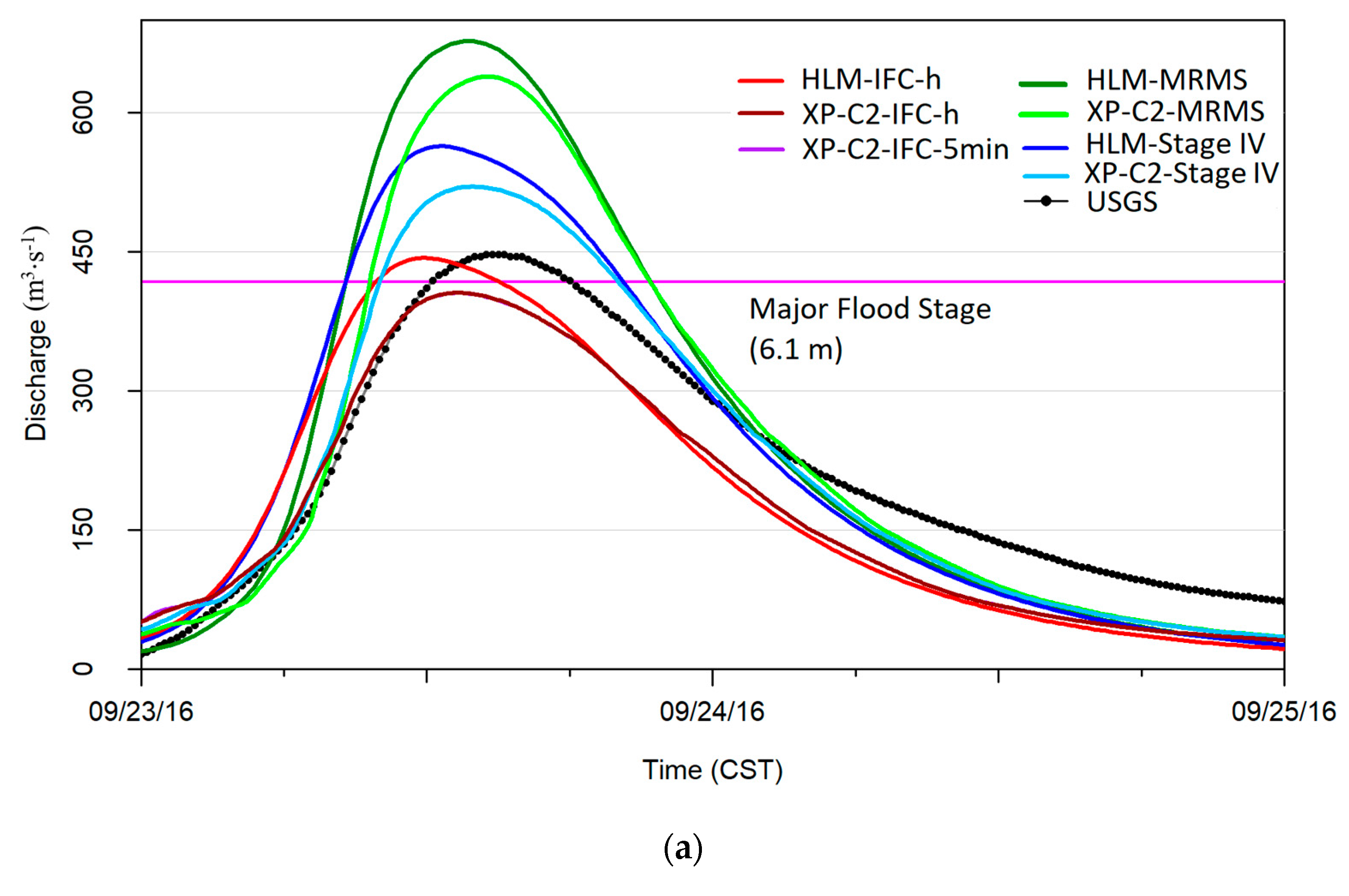
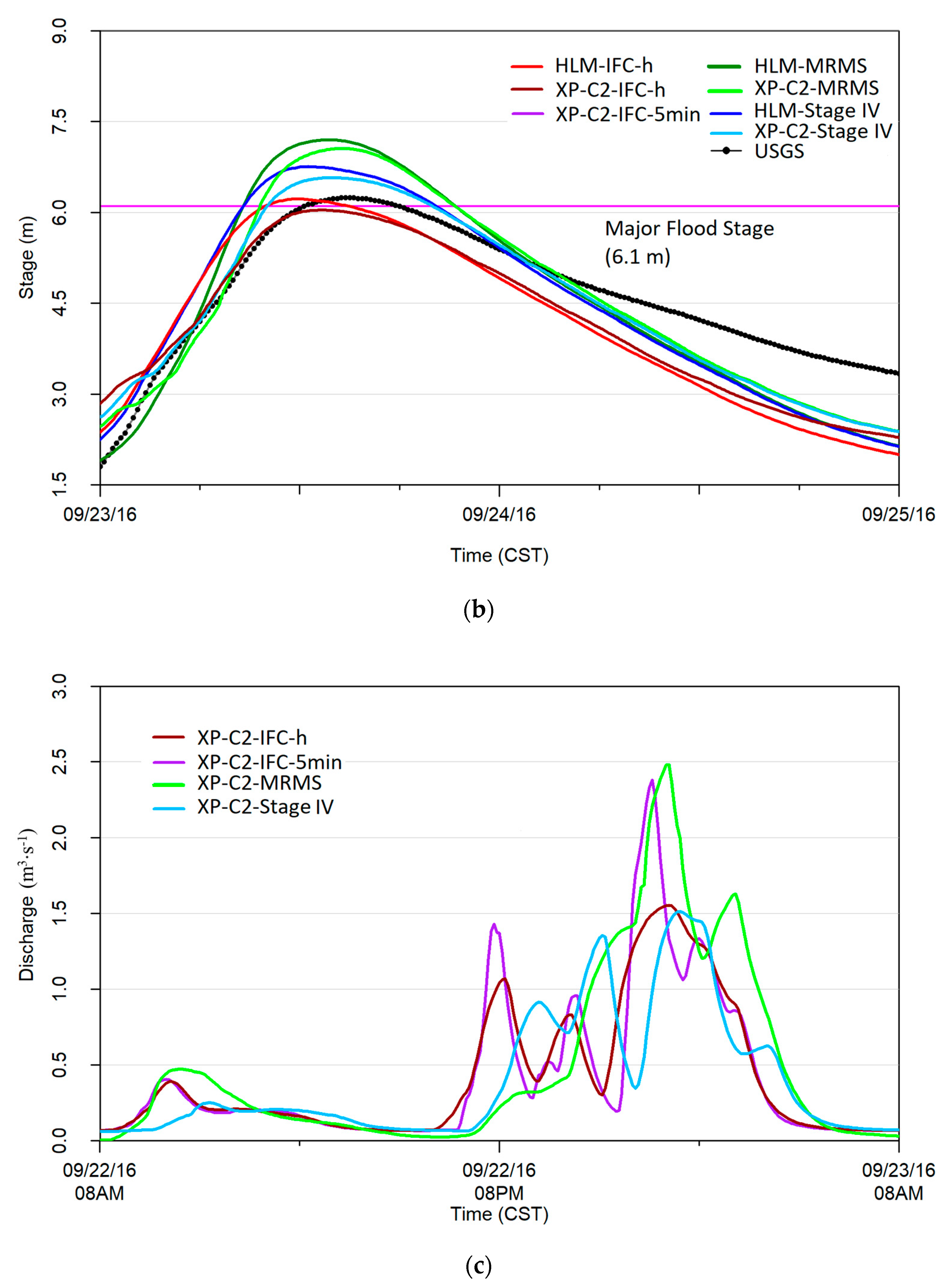
For the September 2016 flood event, the impacts of the varying radar rainfall products on the modeled streamflow were more evident. In
Figure 6a, we can see that the volume of rainfall–runoff differs significantly between each radar rainfall product and the model realizations were arranged as an uncertainty band around the measured values. The impact of the temporal resolution of the IFC radar rainfall estimate was tested for this event but there was no significant change in the results, so much so that the streamflows modeled using IFC 5 minute and IFC hourly overlaid each other, as shown in
Figure 6b. The effect of radar rainfall resolution on the response of the local model was more evidently seen in the streamflow predictions compared to the July 2010 flood.
From the previous experiments, we observed that using hourly and 5 minute IFC rainfall did not considerably change the streamflow predictions at the USGS streamflow gauge on the Maquoketa River. We extracted the flow in the Eastern Tributary to better understand the response of the urban model. In
Figure 6c, it is clear that the higher resolution (both temporal and spatial) of the IFC rainfall product did change the hydrological response of the Eastern Tributary. The IFC 5 minute rainfall allowed for a more detailed description of the transit of flows along the detailed urban drainage network, showing a rising of the hydrographs that could not be obtained with coarser rainfall inputs or coarser hydrological models.
We saw that the models could predict the stage within less than 1 m of error (
Table 3), but none of the models or rainfall inputs significantly outperformed the others. Using the MRMS and Stage IV radar rainfall products, the nested model simulated the major flood level earlier than was observed by 2–3.5 h. It also predicted that the flood duration would be almost double the length of time that was observed. The hourly and 5 min HLM—IFC models generated a hydrograph that was similar in shape and volume to the observed hydrograph. However, the simulations were shifted ahead by 2–3 h because the lower discharge volume produced lower flow velocity in the routing model used by the HLM.
4.3. Modeled Flood Extents
To better understand the performance of the local model as a flood-prediction tool, we evaluated the flood depths and extents from XPSWMM for both historical storms using visual comparison. We primarily looked at the downtown area of Manchester, because this area often experiences nuisance flooding and the city is a point of interest for potential drainage improvement projects. We compared the maximum water depths output from XPSWMM (XP—C2—IFC—h) to photos taken during the flood events. In
Figure 7, it is evident that the local model was able to reproduce the extent of flooding documented in downtown along E Main St. during the July 2010 flood. We have included diamond markers in both the model output and photos to facilitate the comparison. There are elements that reveal similarities between the flood depth map on the top panel and the aerial images; the access to the bridge on E Main St. when traveling west to east is not flooded; the flood depth in the building marked with the blue diamond is approximately half a meter, as indicated in the model output and the imagery.
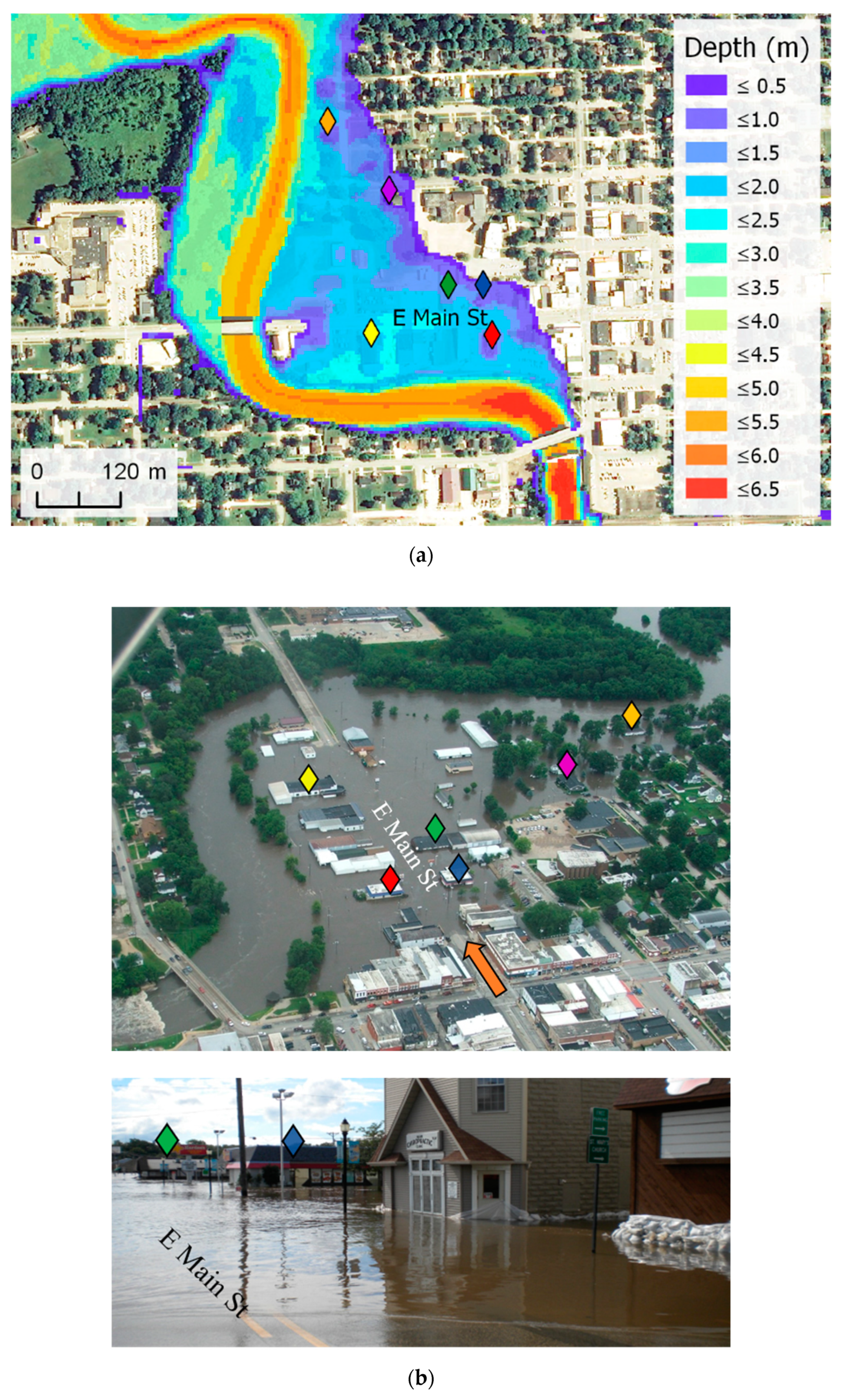
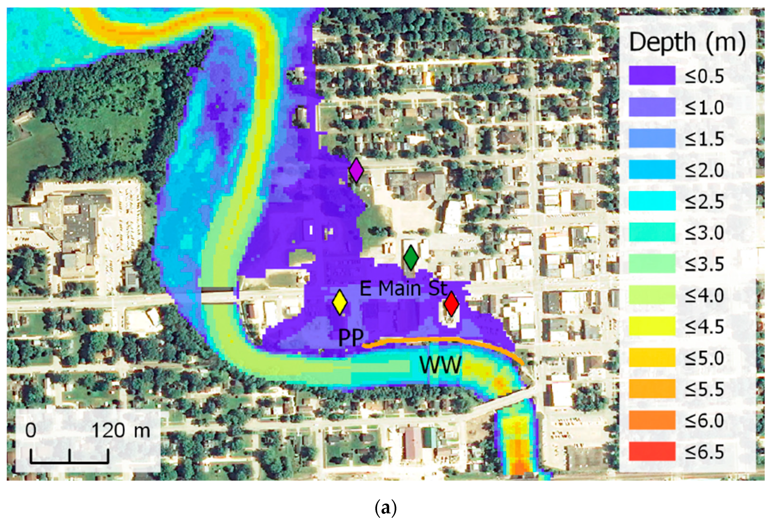
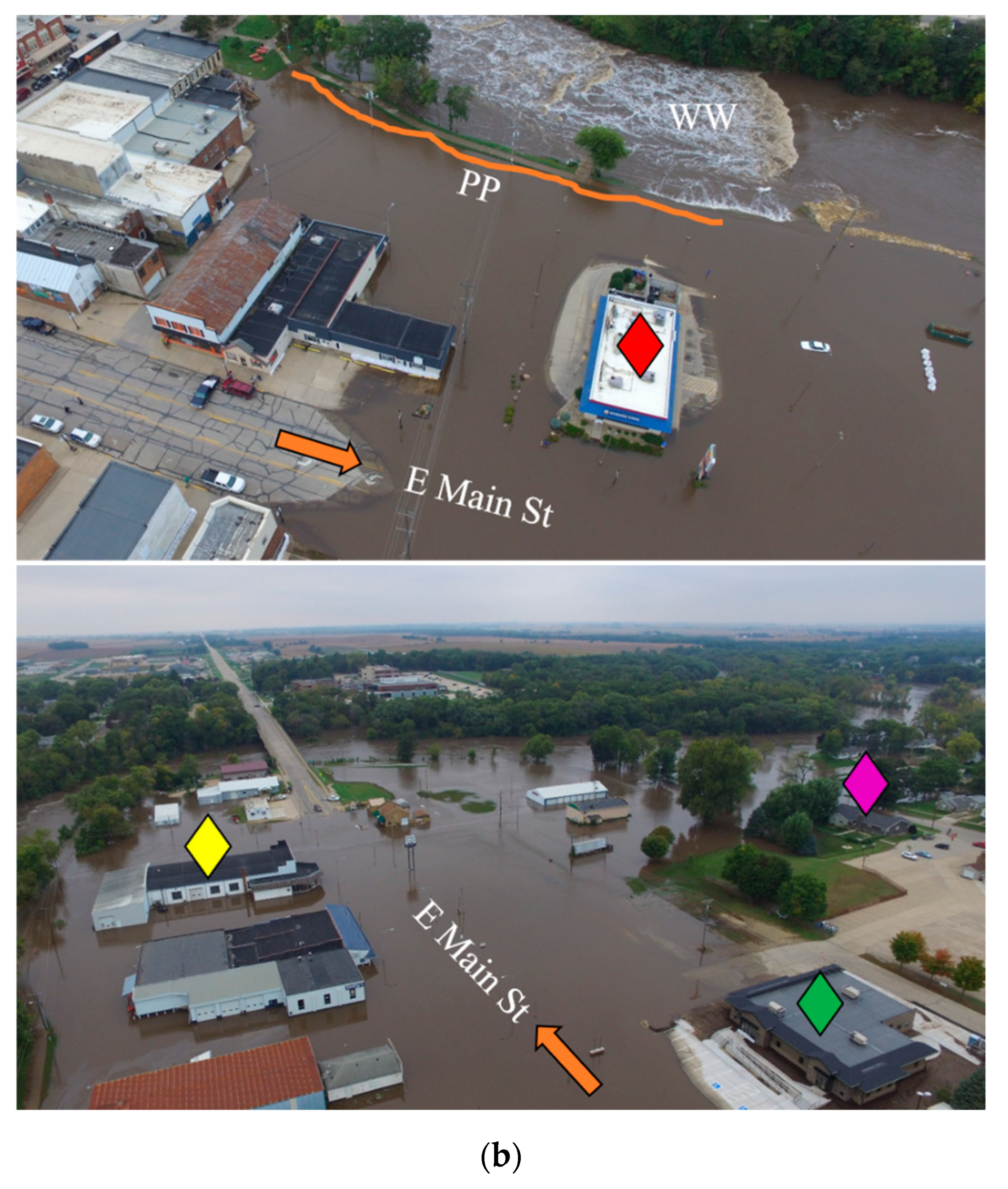
Figure 8 compares the maximum depth outputs from the XPSWMM (XP—C2—Stage IV) model to aerial photos taken for the September 2016 flood. We saw that the model was able to recreate the flow around buildings and the pedestrian path, which acts as an earthen embankment restricting flow into and out of the river. The model correctly estimated the flood depth around the building marked with the red diamond, as an effect of the barrier created by the pedestrian path and the topography. The north side of the building marked in green and the east side of the purple diamond should not be flooded, as indicated by the model and the imagery.
5. Discussion
In this section, we discuss the uncertainty in the data and models and its impacts on the streamflow predictions. We discuss the advantages and disadvantages of the models and the use of a nested regional–local modeling approach.
5.1. Uncertainty and General Observations
Overall, for the two flood events evaluated, the nested modeling approach did not significantly improve the streamflow predictions compared to the regional HLM model. Additional examination is required to determine whether a different configuration of the local model would better resolve the characterization of the hydrograph recession. We evaluated the model’s performance primarily based on its ability to predict stages, because this is important for the city officials to make evacuation decisions. The uncertainty in the observed stages due to errors in the high end of the rating curves propagated into the evaluation of the model results. At extreme flood levels, like the flood of July 2010, the uncertainty associated with rating curves was prominent because we lacked physical measurements to help us quantify the storage of water in the floodplain at high flows. The rating curves traditionally ignore the less-known phenomenon of hysteresis [
62], which is important for large events with unsteady flow. Model parameters are another source of error that will change timing of the watershed response and the volume of runoff produced [
24]. Without in situ measurements, modeling the amount of water that can be stored in the depressions in the land surface, vegetation and canopy, and the soil layers for watersheds with heterogenous terrain and landcover is difficult. There was also uncertainty in the downstream boundary condition, which impacted the ability of the model to reproduce any backwater effects from stormwater management structures or other kinds of impoundments along the floodplain.
The accuracy of the nested approach for use in predicting streamflow is subject to the quality of the regional model and the quality of the finer-resolution data used in the local model. In this study, the uncertainty from the regional inflow applied to the local model was dominant compared to the small volume of runoff from the local model. For fluvial floods, the urban rainfall–runoff dynamics have a negligible impact on total streamflow. However, the impact of radar rainfall spatial and temporal resolution on streamflow predictions was more prominent across the regional model and the nested model. The performance of the nested model simulations did not exhibit systematic characteristics based on the individual rainfall products (e.g., no rainfall product resulted in larger runoff bias, etc.). This draws attention to the large uncertainty in rainfall inputs, which is a result of the non-linear, spatiotemporal patterns of rainfall. However, by using different, equally valid radar rainfall estimates, the ensemble of hydrological predictions envelop the observed hydrograph, thus implicitly accounting for the uncertainty in the radar rainfall input [
63].
5.2. Model Application
Another aim of this work was to test the nested modeling approach to determine whether it is suitable to apply in other areas of the state of Iowa where local models can be one-way coupled to the HLM model, which is actively providing streamflow forecasts [
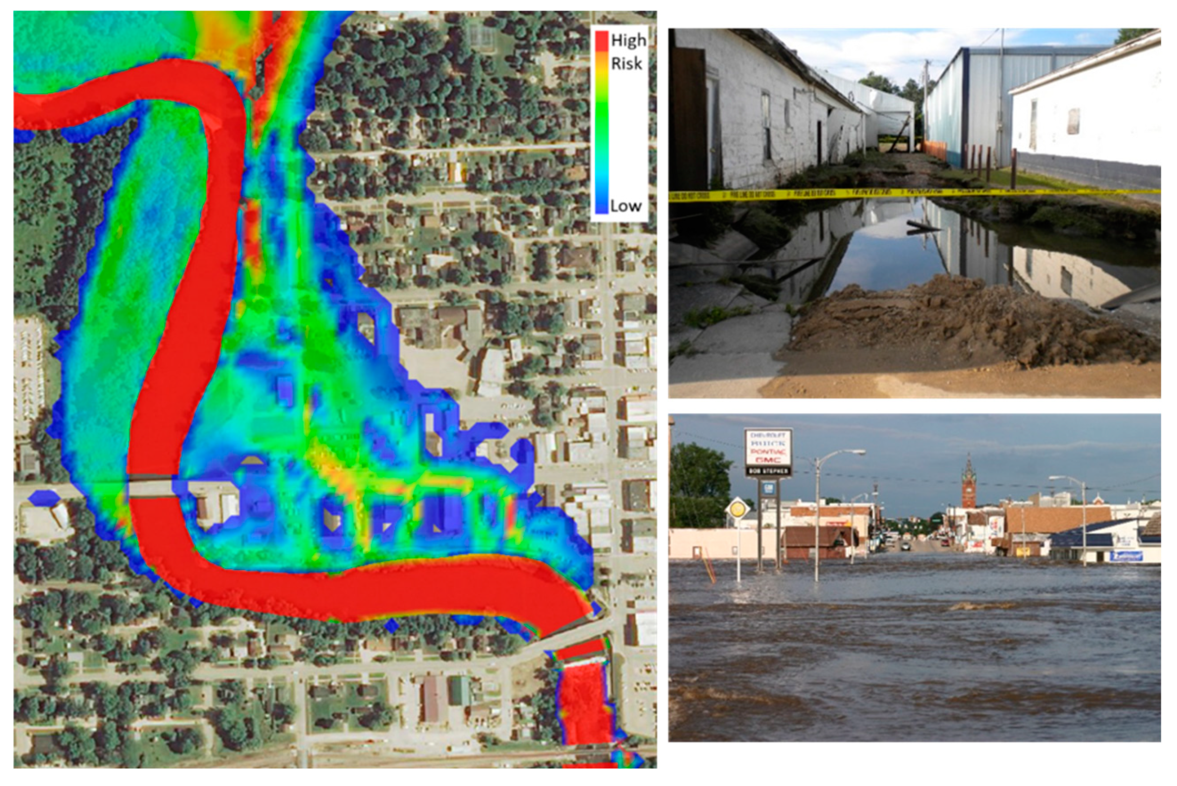
1]. By coupling the regional model to a local model, we can gain additional risk and hazard information that is useful to the local community. Because the XPSWMM model generates velocity and depth information in the 2D domain, we can use these outputs to give emergency responders and local officials hazard maps, such as the one shown in
Figure 9, to support their response. Other kinds of maps that the local hydrodynamic model can produce include road and property safety risk maps, which would aid in making decisions around closing off areas of a city (e.g., E Main St. in downtown Manchester). The XPSWMM model also outputs risk maps that highlight structures that might fail, such as bridges or dams (e.g., the Delhi Dam break).
Since the hydrological importance of the urban rainfall–runoff dynamics is heavily dependent on the volume and intensity of localized rainfall [
64], it is probable that during extreme regional rainfall events, they will have a negligible effect [
65]. For the two historical storms reported in this study, it was the case that the small ungauged tributaries and urban area had a minor impact on the Maquoketa River discharge [
18,
66]. However, by examining the response of the local model with and without subsurface drainage during a local rainfall event in
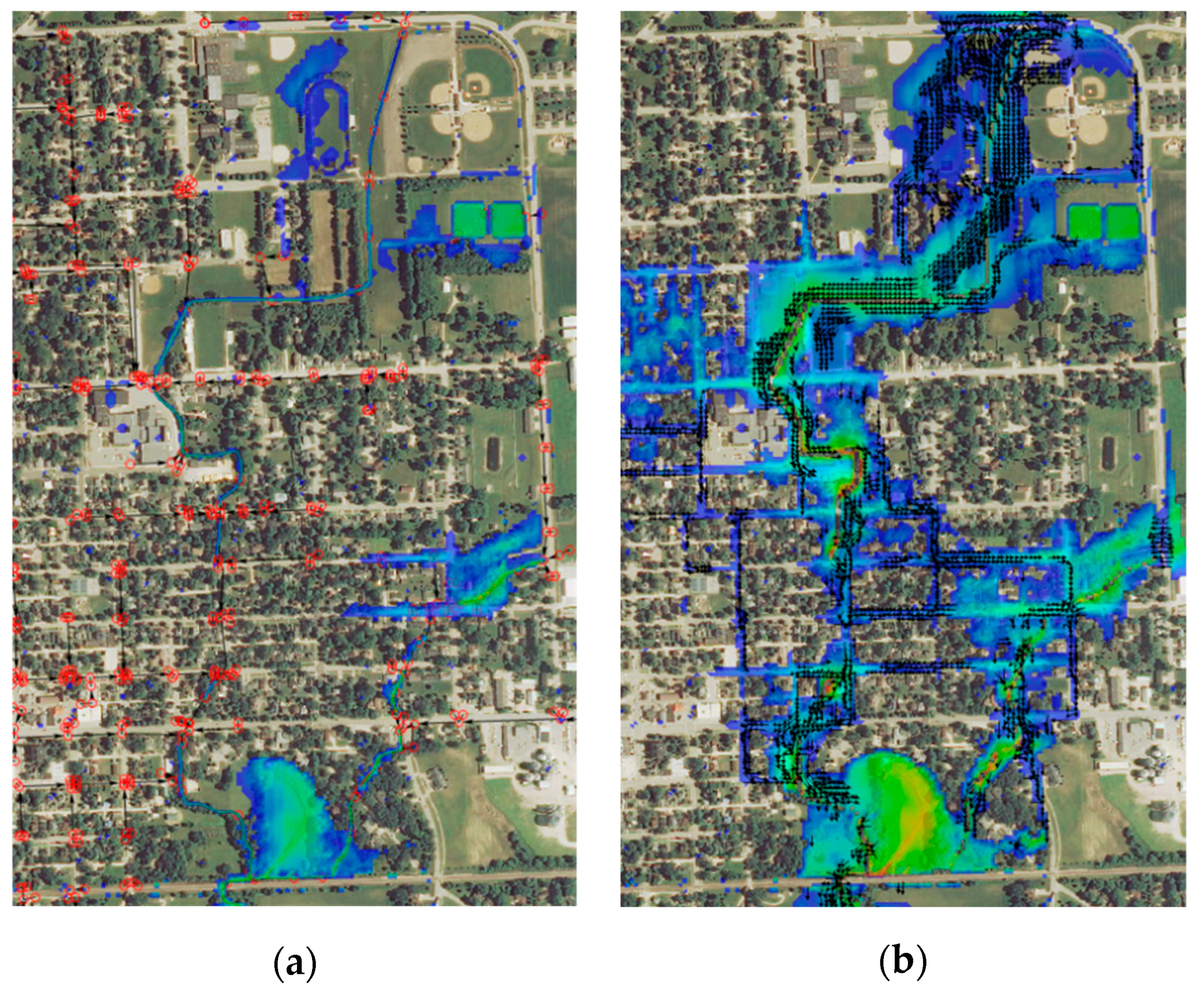
Figure 10, we could see that it is crucial for urban models to be resolved at small spatial scales to better resemble the flow paths in an urban landscape. Ignoring the details of storm sewers and ditches could significantly impact the accuracy of a city’s flood profile for local rainfall events.
6. Conclusions
In this study, we used a nested regional–local model to investigate the impacts of the spatiotemporal resolution of radar rainfall inputs and urban rainfall–runoff dynamics on streamflow predictions in an urban–rural watershed. We applied this modeling approach to the community of Manchester and found that the model was able to predict the flood levels while also providing reasonably accurate forecasts of the magnitude and timing of peak streamflow. The model tended to estimate the peak of the hydrograph slightly earlier than what was observed. Though the model cannot generate a single definitive forecast, it can be used to generate an ensemble of hydrological predictions which are suitable for warning against the worst possible flood. The nested model’s ability to capture the crest time and duration above the NWS major flood stage, despite the various uncertainties in rainfall input, could be used as a tool to assist the community in preparing for potential fluvial and pluvial flooding.
We determined that the hydrological importance of the urban rainfall–runoff dynamics is heavily dependent on a localized rainfall event and intensity. The local urban hydrodynamics do not significantly contribute to streamflow predictions during extreme regional rainfall events, but they are important at smaller tributary basins, where there are fewer observations available for validation. While streamflow outputs from a regional model are necessary for forecasting a riverine-induced flood, ignoring the impacts of the stormwater network could have major implications for the predicted flood risk. During peak river flows, the capacity of the stormwater infrastructure to mitigate any additional local rainfall–runoff would be limited, thus posing a potential flood risk for the urban district.
Capturing the storm movement across a watershed is important for streamflow predictions and the response of the urban drainage system. This study showed how the spatial and temporal variability of radar rainfall inputs will impact streamflow predictions in regional, local, and nested models. For the September 2016 event, the modeled streamflow resulted in various hydrological responses resulting from the varying spatial resolution of the radar rainfall inputs, but it was less sensitive to the temporal resolution. In contrast, for this same storm event, the urban catchment was sensitive to the variations of the radar rainfall inputs in both time and space. Because of the uncertainty associated with radar rainfall estimates, we advocate for using an ensemble hydrological prediction rather than a deterministic approach. By using multiple rainfall forcing and model configurations, we generated an ensemble of model realizations that provide an estimate for the range of potential streamflow observations at the USGS streamflow gauge.
Using a nested modeling approach is an effective method for integrating models built at varying scales. By using a nested modeling approach, we were able to integrate a fine-resolution urban model to a large-scale, simplified model. In doing so, we took advantage of the HLM’s good characterization of regional runoff and XPSWMM’s ability to capture fine-scale flooding in an urban landscape to generate useful flood-relevant information for Manchester. The nested modeling approach adds value to the community because of the detailed flood information (hazard maps, maximum flood depths and extents, etc.) the local model is able to generate at a fine resolution, which can be used to aid decision-makers who need to allocate mitigation resources to high-risk areas.
Author Contributions
Conceptualization, L.E.G. and W.F.K.; methodology, L.E.G. and W.F.K.; software, L.E.G. and F.Q.; validation, L.E.G., F.Q. and W.F.K.; formal analysis, L.E.G.; data curation, L.E.G. and F.Q.; writing—original draft preparation, L.E.G.; writing—review and editing, L.E.G., F.Q. and W.F.K.; visualization, L.E.G.; supervision, W.F.K.; funding acquisition, W.F.K. All authors have read and agreed to the published version of the manuscript.
Funding
This research was funded by the Iowa Flood Center and conducted while L.E.G. was a graduate student at the University of Iowa.
Acknowledgments
Ryan Wicks and others at Fehr and Graham provided data on Manchester’s infrastructure and records of the floods. The local USACE and IDNR agencies provided data, reports, and HEC-RAS models of the Maquoketa River near Manchester.
Conflicts of Interest
The authors declare no conflict of interest.
References
- Krajewski, W.F.; Ceynar, D.; Demir, I.; Goska, R.; Kruger, A.; Langel, C.; Mantilla, R.; Niemeier, J.; Quintero, F.; Seo, B.-C.; et al. Real-time flood forecasting and information system for the state of iowa. Bull. Am. Meteorol. Soc. 2017, 98, 539–554. [Google Scholar] [CrossRef]
- Buchmiller, R.C.; Eash, D.A. Floods of May and June 2008 in Iowa; Iowa Department of Natural Resources: Des Moines, IA, USA, 2010; pp. 1–20.
- Weber, L.J.; Muste, M.; Bradley, A.A.; Amado, A.A.; Demir, I.; Drake, C.W.; Krajewski, W.F.; Loeser, T.J.; Politano, M.S.; Shea, B.R.; et al. The Iowa Watersheds Project: Iowa’s prototype for engaging communities and professionals in watershed hazard mitigation. Int. J. River Basin Manag. 2018, 16, 315–328. [Google Scholar] [CrossRef]
- Quintero, F.; Krajewski, W.F.; Seo, B.-C.; Mantilla, R. Improvement and evaluation of the Iowa Flood Center Hillslope Link Model (HLM) by calibration-free approach. J. Hydrol. 2020, 584, 124686. [Google Scholar] [CrossRef]
- Quintero, F.; Krajewski, W.F.; Mantilla, R.; Small, S.; Seo, B.-C. A Spatial–dynamical framework for evaluation of satellite rainfall products for flood prediction. J. Hydrometeorol. 2016, 17, 2137–2154. [Google Scholar] [CrossRef]
- Schmitt, T.G.; Thomas, M.; Ettrich, N. Analysis and modeling of flooding in urban drainage systems. J. Hydrol. 2004, 299, 300–311. [Google Scholar] [CrossRef]
- Salvadore, E.; Bronders, J.; Batelaan, O. Hydrological modelling of urbanized catchments: A review and future directions. J. Hydrol. 2015, 529, 62–81. [Google Scholar] [CrossRef]
- Mitchell, V.G.; Duncan, H.; Inman, M.; Rahilly, M.; Stewart, J.; Vieritz, A.; Holt, P.; Grant, A.; Fletcher, T.D.; Coleman, J.; et al. State of the Art Review of Integrated Urban Water Models. In Proceedings of the 6th International Conference on Novatech, Lyon, France, 25–28 June 2007. [Google Scholar]
- Knebl, M.R.; Yang, Z.-L.; Hutchison, K.; Maidment, D.R. Regional scale flood modeling using NEXRAD rainfall, GIS, and HEC-HMS/RAS: A case study for the San Antonio River Basin Summer 2002 storm event. J. Environ. Manag. 2005, 75, 325–336. [Google Scholar] [CrossRef]
- Neal, J.C.; Odoni, N.A.; Trigg, M.A.; Freer, J.E.; Garcia-Pintado, J.; Mason, D.C.; Wood, M.; Bates, P.D. Efficient incorporation of channel cross-section geometry uncertainty into regional and global scale flood inundation models. J. Hydrol. 2015, 529, 169–183. [Google Scholar] [CrossRef] [Green Version]
- Salas, F.R.; Somos-Valenzuela, M.A.; Dugger, A.; Maidment, D.R.; Gochis, D.J.; David, C.H.; Yu, W.; Ding, D.; Clark, E.P.; Noman, N. Towards real-time continental scale streamflow simulation in continuous and discrete space. JAWRA J. Am. Water Resour. Assoc. 2018, 54, 7–27. [Google Scholar] [CrossRef]
- Teng, J.; Jakeman, A.J.; Vaze, J.; Croke, B.F.W.; Dutta, D.; Kim, S. Flood inundation modelling: A review of methods, recent advances and uncertainty analysis. Environ. Model. Softw. 2017, 90, 201–216. [Google Scholar] [CrossRef]
- Bisht, D.S.; Chatterjee, C.; Kalakoti, S.; Upadhyay, P.; Sahoo, M.; Panda, A. Modeling urban floods and drainage using SWMM and MIKE URBAN: A case study. Nat. Hazards 2016, 84, 749–776. [Google Scholar] [CrossRef]
- Mark, O.; Weesakul, S.; Apirumanekul, C.; Aroonnet, S.B.; Djordjević, S. Potential and limitations of 1D modelling of urban flooding. J. Hydrol. 2004, 299, 284–299. [Google Scholar] [CrossRef]
- Domingo, N.D.S.; Refsgaard, A.; Mark, O.; Paludan, B. Flood analysis in mixed-urban areas reflecting interactions with the complete water cycle through coupled hydrologic-hydraulic modelling. Water Sci. Technol. 2010, 62, 1386–1392. [Google Scholar] [CrossRef]
- Russo, B.; Sunyer, D.; Velasco, M.; Djordjević, S. Analysis of extreme flooding events through a calibrated 1D/2D coupled model: The case of Barcelona (Spain). J. Hydroinform. 2015, 17, 473–491. [Google Scholar] [CrossRef]
- Chen, A.S.; Evans, B.; Djordjević, S.; Savić, D.A. A coarse-grid approach to representing building blockage effects in 2D urban flood modelling. J. Hydrol. 2012, 426–427, 1–16. [Google Scholar] [CrossRef] [Green Version]
- Bermúdez, M.; Neal, J.C.; Bates, P.D.; Coxon, G.; Freer, J.E.; Cea, L.; Puertas, J. Quantifying local rainfall dynamics and uncertain boundary conditions into a nested regional-local flood modeling system. Water Resour. Res. 2017, 53, 2770–2785. [Google Scholar] [CrossRef] [Green Version]
- Villarini, G.; Krajewski, W.F. Review of the different sources of uncertainty in single polarization radar-based estimates of rainfall. Surv. Geophys. 2010, 31, 107–129. [Google Scholar] [CrossRef]
- Wright, D.B.; Smith, J.A.; Villarini, G.; Baeck, M.L. Long-term high-resolution radar rainfall fields for urban hydrology. JAWRA J. Am. Water Resour. Assoc. 2014, 50, 713–734. [Google Scholar] [CrossRef]
- Emmanuel, I.; Andrieu, H.; Leblois, E.; Janey, N.; Payrastre, O. Influence of rainfall spatial variability on rainfall-runoff modelling: Benefit of a simulation approach? J. Hydrol. 2015, 531, 337–348. [Google Scholar] [CrossRef]
- Ochoa-Rodriguez, S.; Wang, L.P.; Gires, A.; Pina, R.D.; Reinoso-Rondinel, R.; Bruni, G.; Ichiba, A.; Gaitan, S.; Cristiano, E.; Van Assel, J.; et al. Impact of spatial and temporal resolution of rainfall inputs on urban hydrodynamic modelling outputs: A multi-catchment investigation. J. Hydrol. 2015, 531, 389–407. [Google Scholar] [CrossRef]
- Krajewski, W.F.; Kruger, A.; Singh, S.; Seo, B.-C.; Smith, J.A. Hydro-NEXRAD-2: Real-time access to customized radar-rainfall for hydrologic applications. J. Hydroinform. 2013, 15, 580–590. [Google Scholar] [CrossRef]
- Smith, B.K.; Smith, J.A.; Baeck, M.L.; Villarini, G.; Wright, D.B. Spectrum of storm event hydrologic response in urban watersheds. Water Resour. Res. 2013, 49, 2649–2663. [Google Scholar] [CrossRef]
- Bruni, G.; Reinoso, R.; Van de Giesen, N.C.; Clemens, F.H.L.R.; Ten Veldhuis, J.A.E. On the sensitivity of urban hydrodynamic modelling to rainfall spatial and temporal resolution. Hydrol. Earth Syst. Sci. 2015, 19, 691–709. [Google Scholar] [CrossRef] [Green Version]
- Wang, L.-P.; Ochoa-Rodríguez, S.; Van Assel, J.; Pina, R.D.; Pessemier, M.; Kroll, S.; Willems, P.; Onof, C. Enhancement of radar rainfall estimates for urban hydrology through optical flow temporal interpolation and Bayesian gauge-based adjustment. J. Hydrol. 2015, 531, 408–426. [Google Scholar] [CrossRef] [Green Version]
- Thorndahl, S.; Einfalt, T.; Willems, P.; Nielsen, J.E.; Ten Veldhuis, M.-C.; Arnbjerg-Nielsen, K.; Rasmussen, M.R.; Molnar, P. Weather radar rainfall data in urban hydrology. Hydrol. Earth Syst. Sci. 2017, 21, 1359–1380. [Google Scholar] [CrossRef] [Green Version]
- Peleg, N.; Blumensaat, F.; Molnar, P.; Fatichi, S.; Burlando, P. Partitioning the impacts of spatial and climatological rainfall variability in urban drainage modeling. Hydrol. Earth Syst. Sci. 2017, 21, 1559–1572. [Google Scholar] [CrossRef] [Green Version]
- Fletcher, T.D.; Andrieu, H.; Hamel, P. Understanding, management and modelling of urban hydrology and its consequences for receiving waters: A state of the art. Adv. Water Resour. 2013, 51, 261–279. [Google Scholar] [CrossRef]
- Liu, Y.; Gupta, H.V. Uncertainty in hydrologic modeling: Toward an integrated data assimilation framework. Water Resour. Res. 2007, 43. [Google Scholar] [CrossRef]
- Eash, D.A. Floods of July 23–26, 2010, in the Little Maquoketa River and Maquoketa River Basins, Northeast Iowa; Open-File Report 2011-1301; U.S. Geological Survey: Reston, VI, USA, 2012.
- Innovyze. XPSWMM Reference Manual; XPSWMM and XPStorm Resource Center: Portland, OR, USA, 2016. [Google Scholar]
- Small, S.J.; Jay, L.O.; Mantilla, R.; Curtu, R.; Cunha, L.K.; Fonley, M.; Krajewski, W.F. An asynchronous solver for systems of ODEs linked by a directed tree structure. Adv. Water Resour. 2013, 53, 23–32. [Google Scholar] [CrossRef]
- USDA. Natural Resources Conservation Service Web Soil Survey. Available online: http://websoilsurvey.nrcs.usda.gov/ (accessed on 20 July 2017).
- Knighton, J.; White, E.; Lennon, E.; Rajan, R. Development of probability distributions for urban hydrologic model parameters and a Monte Carlo analysis of model sensitivity. Hydrol. Process. 2014, 28, 5131–5139. [Google Scholar] [CrossRef]
- Rawls, W.J.; Brakensiek, D.L.; Miller, N. Green-ampt infiltration parameters from soils data. J. Hydraul. Eng. 1983, 109, 62–70. [Google Scholar] [CrossRef] [Green Version]
- Iowa Geodata. Available online: https://geodata.iowa.gov/dataset/high-resolution-land-cover-iowa-2009-564 (accessed on 20 July 2017).
- Arrault, A.; Finaud-Guyot, P.; Archambeau, P.; Bruwier, M.; Erpicum, S.; Pirotton, M.; Dewals, B. Hydrodynamics of long-duration urban floods: Experiments and numerical modelling. Nat. Hazards Earth Syst. Sci. 2016, 16, 1413–1429. [Google Scholar] [CrossRef] [Green Version]
- USDA. National Resources Conservation Service: Manning’s (Roughness) Coefficient. Available online: https://www.nrcs.usda.gov/wps/portal/nrcs/detail/national/water/manage/hydrology/?cid=stelprdb104570 (accessed on 20 July 2017).
- Brown, J.D.; Spencer, T.; Moeller, I. Modeling storm surge flooding of an urban area with particular reference to modeling uncertainties: A case study of Canvey Island, United Kingdom. Water Resour. Res. 2007, 43, 1–22. [Google Scholar] [CrossRef] [Green Version]
- Syme, W.J. Flooding in urban areas–2d modelling approaches for buildings and fences. In Proceedings of the Engineers Australia 9th National Conference on Hydraulics in Water Engineering, Darwin, Australia, 23 September 2008. [Google Scholar]
- Schubert, J.E.; Sanders, B.F. Building treatments for urban flood inundation models and implications for predictive skill and modeling efficiency. Adv. Water Resour. 2012, 41, 49–64. [Google Scholar] [CrossRef]
- Smith, G.P.; Wasko, C.D.; Miller, B.M. Modelling the influence of buildings on flood flow. In Proceedings of the 52th Floodplain Management National Conference, Batemans Bay, Australia, 21–24 February 2012. [Google Scholar]
- Bellos, V.; Tsakiris, G. Comparing various methods of building representation for 2D flood modelling in built-up areas. Water Resour. Manag. 2015, 29, 379–397. [Google Scholar] [CrossRef]
- Gironás, J.; Niemann, J.D.; Roesner, L.A.; Rodriguez, F.; Andrieu, H. Evaluation of methods for representing urban terrain in stormwater modeling. J. Hydrol. Eng. 2010, 15, 14. [Google Scholar] [CrossRef] [Green Version]
- Jankowfsky, S.; Branger, F.; Braud, I.; Gironás, J.; Rodriguez, F. Comparison of catchment and network delineation approaches in complex suburban environments: Application to the Chaudanne catchment, France. Hydrol. Process. 2013, 27, 3747–3761. [Google Scholar] [CrossRef] [Green Version]
- Rodriguez, F.; Bocher, E.; Chancibault, K. Terrain representation impact on periurban catchment morphological properties. J. Hydrol. 2013, 485, 54–67. [Google Scholar] [CrossRef]
- Mignot, E.; Paquier, A.; Haider, S. Modeling floods in a dense urban area using 2D shallow water equations. J. Hydrol. 2006, 327, 186–199. [Google Scholar] [CrossRef] [Green Version]
- Fewtrell, T.J.; Bates, P.D.; Horritt, M.; Hunter, N.M. Evaluating the effect of scale in flood inundation modelling in urban environments. Hydrol. Process. 2008, 22, 5107–5118. [Google Scholar] [CrossRef]
- Zhang, J.; Howard, K.; Langston, C.; Kaney, B.; Qi, Y.; Tang, L.; Grams, H.; Wang, Y.; Cocks, S.; Martinaitis, S.; et al. Multi-Radar Multi-Sensor (MRMS) quantitative precipitation estimation: Initial operating capabilities. Bull. Am. Meteorol. Soc. 2016, 97, 621–638. [Google Scholar] [CrossRef]
- Lin, Y.; Mitchell, K.E. The NCEP Stage II/IV hourly precipitation analyses: Development and applications. In Proceedings of the Preprints 19th Conference on Hydrology, American Meteorological Society, San Diego, CA, USA, 9–13 January 2005; pp. 2–5. [Google Scholar]
- Seo, B.-C.; Krajewski, W.F.; Quintero, F.; ElSaadani, M.; Goska, R.; Cunha, L.K.; Dolan, B.; Wolff, D.B.; Smith, J.A.; Rutledge, S.A.; et al. Comprehensive evaluation of the ifloods radar rainfall products for hydrologic applications. J. Hydrometeorol. 2018, 19, 1793–1813. [Google Scholar] [CrossRef]
- Seo, B.C.; Krajewski, W.F. Correcting temporal sampling error in radar-rainfall: Effect of advection parameters and rain storm characteristics on the correction accuracy. J. Hydrol. 2015, 531, 272–283. [Google Scholar] [CrossRef]
- Seo, B.C.; Krajewski, W.F.; Mishra, K.V. Using the new dual-polarimetric capability of WSR-88D to eliminate anomalous propagation and wind turbine effects in radar-rainfall. Atmos. Res. 2015, 153, 296–309. [Google Scholar] [CrossRef]
- Iowa State University Iowa Environmental Mesonet. Available online: https://mesonet.agron.iastate.edu/sites/locate.php (accessed on 15 August 2017).
- Krause, P.; Boyle, D.P.; Bäse, F. Comparison of different efficiency criteria for hydrological model assessment. Adv. Geosci. 2005, 5, 89–97. [Google Scholar] [CrossRef] [Green Version]
- Reusser, D.E.; Blume, T.; Schaefli, B.; Zehe, E. Analysing the temporal dynamics of model performance for hydrological models. Hydrol. Earth Syst. Sci. 2009, 13, 999–1018. [Google Scholar] [CrossRef] [Green Version]
- Legates, D.R.; McCabe, G.J. Evaluating the use of “goodness-of-fit” Measures in hydrologic and hydroclimatic model validation. Water Resour. Res. 1999, 35, 233–241. [Google Scholar] [CrossRef]
- Jachner, S.; Boogaart, G.; Petzoldt, T. Statistical methods for the qualitative assessment of dynamic models with time delay (R Package qualV). J. Stat. Softw. 2007, 22. [Google Scholar] [CrossRef] [Green Version]
- Zalenski, G.; Krajewski, W.F.; Quintero, F.; Restrepo, P.; Buan, S. Analysis of national weather service stage forecast errors. Weather Forecast. 2017, 32, 1441–1465. [Google Scholar] [CrossRef]
- Fiedler, W.; King, W.; Schwanz, N. Independent Panel of Engineers: Report on Breach of Delhi Dam; Iowa Department of Natural Resources: Des Moines, IA, USA, 2010.
- Lee, K.; Firoozfar, A.R.; Muste, M. Technical Note: Monitoring of unsteady open channel flows using the continuous slope-area method. Hydrol. Earth Syst. Sci. 2017, 21, 1863–1874. [Google Scholar] [CrossRef]
- Quintero, F.; Sempere-Torres, D.; Berenguer, M.; Baltas, E. A scenario-incorporating analysis of the propagation of uncertainty to flash flood simulations. J. Hydrol. 2012, 460–461, 90–102. [Google Scholar] [CrossRef]
- Javier, J.R.N.; Smith, J.A.; Meierdiercks, K.L.; Baeck, M.L.; Miller, A.J. Flash flood forecasting for small urban watersheds in the baltimore metropolitan region. Weather Forecast. 2007, 22, 1331–1344. [Google Scholar] [CrossRef]
- Ogden, F.L.; Raj Pradhan, N.; Downer, C.W.; Zahner, J.A. Relative importance of impervious area, drainage density, width function, and subsurface storm drainage on flood runoff from an urbanized catchment. Water Resour. Res. 2011, 47, 1–12. [Google Scholar] [CrossRef] [Green Version]
- Neal, J.; Schumann, G.; Bates, P. A subgrid channel model for simulating river hydraulics and floodplain inundation over large and data sparse areas. Water Resour. Res. 2012, 48, 1–16. [Google Scholar] [CrossRef]
Figure 1.
(a) The extent of the regional model was 725 km2 of rural land in the upper Maquoketa River watershed, located in northeast Iowa. The major tributaries are Coffins Creek and Honey Creek, which drain into the Maquoketa River at the north end of the city limits of Manchester. (b) The extent of the local model included Manchester city limits, which are divided by the Maquoketa River. The Eastern Tributary drains into the Maquoketa River near the United State Geological Survey USGS streamflow gauge and NWS Coop rain gauge located at the model outlet.
Figure 2.
(a) The observed discharge in units of m3⋅s−1 (black dots) at the USGS streamflow gauge on the Maquoketa River at Manchester during the July 2010 flood, with hourly Stage IV radar rainfall intensity time series in mm⋅h−1 (black vertical bars) and the three NWS flood stage categories (horizontal colored lines) (b) the September 2016 flood.
Figure 3.
(a) The flow diagram of the nested regional–local model approach used to test the sensitivity of the streamflow predictions to various radar rainfall products and urban hydrodynamics. (b) The local XPSWMM model (XP—C2) included the green rainfall–runoff subcatchments, and their connections to the 2D domain (gray) are noted by green triangles. The blue triangles are the locations where the regional HLM streamflow is input into the XPSWMM model. The nested model and regional model outputs were compared to observations at the USGS streamflow gauge (yellow squares). The blue polylines (river network) were modeled by the HLM while the black polylines (river and urban drainage network) are modeled in XPSWMM.
Figure 4.
(a) Radar rainfall accumulation estimates over the upper Maquoketa River Basin in mm for the July 2010 storm using Stage IV radar rainfall product (left) and the Iowa Flood Center (IFC) radar rainfall product (right). (b) Radar rainfall accumulation estimates for the September 2016 storm using Stage IV (left) and MRMS radar rainfall product (right).
Figure 5.
The modeled discharge (m3⋅s−1) and stage (m) compared to (a) USGS stage and (b) discharge observations for July 2010. The simulated hydrographs are named according to the model (HLM or XP-C2) and the radar rainfall input. The models forced with the IFC hourly radar rainfall product are red (simulations HLM—FC—h and XP—C2—IFC—h) while those forced with Stage IV hourly radar rainfall are blue (simulations HLM—Stage IV and XP—C2—Stage IV).
Figure 6.
The modeled discharge (m3⋅s−1) and stage (m) compared to (a) USGS stage and (b) discharge observations for September 2016. The simulated hydrographs are named according to the model (HLM or XP—C2) and the radar rainfall input. The models forced with the IFC hourly radar rainfall product are red (HLM—IFC—h, XP—C2—IFC—h, XP—C2—IFC—5min) while those forced with Stage IV hourly radar rainfall are blue (HLM—Stage IV and XP—C2—Stage IV). Models forced with MRMS hourly radar rainfall are colored green (HLM—MRMS and XP—C2—MRMS). (c) The discharge from the Eastern Tributary, which drains the eastern domain of the XPSWMM model, shows how the hydrological response of Manchester is significantly impacted by the spatial and temporal resolution of the radar rainfall input.
Figure 7.
The nested model was used to simulate the flood of July 2010 in downtown Manchester. (a) The maximum depth output from XPSWMM (XP—C2—IFC—h) was compared visually to (b) photos and aerial images of flooding provided by the City of Manchester. The points of interest are indicated by colored diamond markers on both the photos and flood map. The orange arrow is pointing in the westbound direction along E Main Street.
Figure 8.
The nested model was used to simulate the flood of September 2016 in downtown Manchester. (a) The maximum depth output from XPSWMM (XP—C2—Stage IV) was compared to (b) photos and aerial images of flooding provided by the City of Manchester. The points of interest are indicated by colored diamond markers on both the photos and flood map. The orange arrow is pointing in the westbound direction along E Main Street. The newly built whitewater park in the Maquoketa River is labeled as WW and the pedestrian path (orange line labeled PP) is shown to impede stormwater flow from downtown into the river.
Figure 9.
Maximum hazard map output from XPSWMM (XP—C2—IFC—h) for the July 2010 flood event, where red indicates high risk and blue is low risk (risk is a function of water depth and velocity computed in the model). Photos from the July 2010 flood event provided by the city show scour in between buildings and turbulent flow through downtown streets.
Figure 10.
The maximum flood depths in Eastern Manchester for a heavy local rainfall event using the XPSWMM model where (
a) has the stormwater system (described in
Section 3.2) activated and (
b) is overland flow only.
Figure 10.
The maximum flood depths in Eastern Manchester for a heavy local rainfall event using the XPSWMM model where (
a) has the stormwater system (described in
Section 3.2) activated and (
b) is overland flow only.
Table 1.
Cumulative radar rainfall (mm) computed over Manchester using Stage IV, MRMS, and IFC products and the maximum rainfall intensity (mm⋅h−1) for the July 2010 and September 2016 storms. The daily rainfall measurements from the NWS Coop rain gauge data near Manchester were compared to the radar rainfall estimates.
| | July 2010 Storm | September 2016 Storm |
|---|
| Product | Cumulative Rainfall (mm) | Max Rainfall Intensity (mm⋅h−1) | Cumulative Rainfall (mm) | Max Rainfall Intensity (mm⋅h−1) |
|---|
| Stage IV | 196 | 36 | 157 | 28 |
| MRMS | --- | --- | 157 | 33 |
| IFC | 224 | 43 | 168 | 28 |
| NWS Coop rain gauge | 185 | --- | 145 | --- |
Table 2.
Statistical analysis comparing the simulated stages to USGS observations for the first and second peaks of the July 2010 flood and the time to crest and the duration above the NWS major flood stage (6.1 m) for the first peak for model configurations HLM and XP—C2, using both Stage IV and IFC radar rainfall products.
| Rainfall | Model | RMSE (m) | MAE (m) | R2 | PE (m) | TPE (h) | Time to Crest 6.1 m Error (h) | Duration above 6.1 m Error (h) |
|---|
| Peak 1 | | | | | | | | |
| Stage IV | HLM | 0.32 | 0.28 | 0.98 | −0.04 | 2.8 | −1.0 | −6.3 |
| | XP—C2 | 0.30 | 0.23 | 0.99 | 0.10 | 2.0 | 0.3 | −8.3 |
| IFC—h | HLM | 0.43 | 0.39 | 0.98 | −0.30 | 2.8 | 0.5 | −5.5 |
| | XP—C2 | 0.49 | 0.41 | 0.97 | −0.11 | 1.3 | 1.5 | −6.3 |
| Peak 2 | | | | | | | | |
| Stage IV | HLM | 1.5 | 1.4 | 0.99 | 1.17 | 9.3 | | |
| | XP—C2 | 1.6 | 1.5 | 0.99 | 1.17 | 9.3 | | |
| IFC—h | HLM | 1.3 | 1.2 | 0.99 | 0.62 | −4.3 | | |
| | XP—C2 | 1.4 | 1.3 | 0.99 | 0.73 | −4.8 | | |
Table 3.
Statistical analysis comparing the simulated stages to USGS observations for the September 2016 flood, and the time to crest and the duration above the NWS major flood stage (6.1 m) for model configurations HLM and XP—C2 using Stage IV, MRMS, and IFC (hourly and 5 min) radar rainfall products.
| Rainfall | Model | RMSE (m) | MAE (m) | R2 | PE (m) | TPE (h) | Time to Crest 6.1 m Error (h) | Duration above 6.1 m Error (h) |
|---|
| Stage IV | HLM | 0.7 | 0.6 | 0.89 | −0.51 | 2.0 | −3.5 | 5.5 |
| | XP—C2 | 0.6 | 0.5 | 0.88 | −0.33 | 0.5 | −2.2 | 4.2 |
| MRMS | HLM | 0.7 | 0.6 | 0.88 | −0.96 | 0.8 | −3.5 | 6.8 |
| | XP—C2 | 0.6 | 0.5 | 0.90 | −0.81 | 0.0 | −2.6 | 5.9 |
| IFC—5 min | HLM | 0.8 | 0.6 | 0.89 | 0.02 | 2.5 | −2.3 | −0.8 |
| | XP—C2 | 0.7 | 0.6 | 0.88 | 0.20 | 1.3 | --- | --- |
| IFC—h | XP—C2 | 0.7 | 0.6 | 0.84 | 0.20 | 1.3 | --- | --- |
© 2020 by the authors. Licensee MDPI, Basel, Switzerland. This article is an open access article distributed under the terms and conditions of the Creative Commons Attribution (CC BY) license (http://creativecommons.org/licenses/by/4.0/).


