New Numerical Results for the Time-Fractional Phi-Four Equation Using a Novel Analytical Approach
by
 , , and
Wei Gao
1,*, 
Pundikala Veeresha
2 ,
,
Doddabhadrappla Gowda Prakasha
3,
Haci Mehmet Baskonus
4 and
Gulnur Yel
5 1
School of Information Science and Technology, Yunnan Normal University, Kunming 650500, China
2
Department of Mathematics, Karnatak University, Dharwad 580003, India
3
Department of Mathematics, Faculty of Science, Davangere University, Shivagangothri, Davangere 577007, India
4
Department of Mathematics and Science Education, Faculty of Education, Harran University, Sanliurfa 63200, Turkey
5
Faculty of Educational Sciences, Final International University, Mersin 10, Kyrenia 99370, Turkey
*
Author to whom correspondence should be addressed.
Symmetry 2020, 12(3), 478; https://doi.org/10.3390/sym12030478
Submission received: 13 February 2020
/
Revised: 5 March 2020
/
Accepted: 6 March 2020
/
Published: 19 March 2020
(This article belongs to the Special Issue Symmetry and Complexity 2020)
Abstract
:This manuscript investigates the fractional Phi-four equation by using -homotopy analysis transform method (-HATM) numerically. The Phi-four equation is obtained from one of the special cases of the Klein-Gordon model. Moreover, it is used to model the kink and anti-kink solitary wave interactions arising in nuclear particle physics and biological structures for the last several decades. The proposed technique is composed of Laplace transform and -homotopy analysis techniques, and fractional derivative defined in the sense of Caputo. For the governing fractional-order model, the Banach’s fixed point hypothesis is studied to establish the existence and uniqueness of the achieved solution. To illustrate and validate the effectiveness of the projected algorithm, we analyze the considered model in terms of arbitrary order with two distinct cases and also introduce corresponding numerical simulation. Moreover, the physical behaviors of the obtained solutions with respect to fractional-order are presented via various simulations.
1. Introduction
Recently, many new fractional-order operator types have been introduced to the literature by some scholars, and established its fundamental properties [1,2,3,4,5,6]. Fractional theory is widely used to explain many properties of phenomena such as nanotechnology [7], optics [8], human diseases [9], chaos theory [10], and others [11,12,13,14,15,16,17,18,19,20,21,22,23,24,25,26,27,28,29,30,31,32]. As an example, the tumor-immune surveillance model has been investigated in [33]. Some important properties of dengue fever have been effectively investigated in [34,35]. The analytical as well as numerical solutions for the equations illustrating the above cited phenomena, have an important role in describing the behavior of nonlinear models ascends [36,37,38,39,40]. For the differential equation, symmetry is a transformation that keeps its family of solutions invariant, and further, its analysis can be applied to examine and illustrate various classes of differential equations. The study of fractional calculus associated to symmetry recently attracted many researchers from different disciplines in order to present their viewpoints while analyzing real-word problems.
The Klein-Gordon (KG) equation is derived by physicists Klein and Gordon to investigate the behavior of relativistic electrons. As a specific form of the KG equation, the Phi-four equation is defined to illustrate wave interactions [41,42] which is considered as in fractional order, namely, fractional Phi-four (FPF) equation
with
Here, and are real-valued constants. Here, is the normalized propagation of distance and retracted time .
Many physicists and mathematicians recently proposed very accurate and more effective algorithms to find and examine the solution for equations describing nonlinear mechanisms arising in science and engineering. As an approximate method, the homotopy analysis method (HAM) has been introduced by L. Shijun [43,44], which is formed to describe deformation from zero to 1. Recently, it has been efficiently and beneficially employed to examine the nature of nonlinear problems without linearization and perturbation. However, HAM necessitates huge time and computer memory for computational work. Therefore, there is an essence of the consolidation of this scheme with familiar transform algorithms. The projected solution procedure is the mixture of -HAM with LT [45]. Since the future scheme is a modified method of HAM, it does not kernel discretization, perturbation or linearization [46,47,48,49,50,51,52,53,54,55,56].
The considered nonlinear problem recently fascinated authors from various areas of science. Due to the numerous applications of the proposed model and the important role it plays in describing various nonlinear phenomena, several researchers found and investigated the solution numerically and also analytically; for instance, researchers in [57] find the new exact solution for the fractional case of considered nonlinear problem, and the spectral collocation method is considered in [58] to find the solution for PF equation. The considered nonlinear PF equation has attracted the attention of researchers, and, in order to present their viewpoint, many techniques are considered [59,60,61,62,63,64,65], presenting some interesting results. Recently many researchers from all over the world have investigated Fractional Calculus (FC) as an effective tool by comparing with other operators some important physical problems [66,67,68,69,70,71,72,73,74,75,76,77,78,79]. For instance, authors in [80] presented the reflection symmetry in fractional calculus, and proposed some interesting properties and corresponding consequences.
The main aim of this paper is to investigate the numerical solutions for the considered fractional Phi-Four equation using the novel technique. The proposed algorithm provides more liberty to consider the diverse class complex as well as nonlinear problems and the initial guess.
In this paper, we try to capture in the physical behaviors obtained numerical solutions with distinct arbitrary order and the parameters accessible by the projected algorithm. Moreover, in order to present accuracy and effectiveness, we present the numerical simulations. By the help of these results, we try to explain the diverse model exemplifying numerous phenomena arising in daily life. The rest of the paper is organized as follows: the basic properties of FC are presented in Section 2, the basic solution algorithm of the projected method for the considered problem is defined in Section 3, the convergence analysis of the considered scheme is illustrated in Section 4, the solution for FPF equation and its corresponding consequences in terms plots and also numerical simulation are respectively cited in Section 5 and Section 6. Finally, some important findings of the paper are presented as a conclusion section.
2. Preliminaries
In this subsection of the paper, it is presented the basic definitions of fractional calculus.
Definition 1.
Fractional integral ofwith the orderis defined in RL as
Definition 2.
Fractional derivative ofis given in the sense of Caputo as the following:
Definition 3.
The Laplace transform (LT) offor a Caputo fractional derivative is introduced as below:
whereis LT of.
3. Solution Procedure for Fractional Phi-Four Equation
Here, we consider the nonlinear FPF equation to illustrate the basic solution algorithm of the projected method with associated initial conditions as follows:
and
Here, signifies the fractional Caputo-derivative of Here, is a bounded function. On using the LT on Equation (5), and then by the help of Equation (6), it is given as following
By the assist of Equation (7), the nonlinear operator is given as follows:
Now, the homotopy structure is defined by
where and are respectively the embedding and auxiliary parameter. Further, these parameters help us to control and adjust the convergence region of the obtained solution. For the proper choice of and , the obtained solution quickly converges to the exact solution in an admissible domain. The following results are respectively true for and
Near to , we define in series form by help of the Taylor theorem and then one can obtain
where
For the proper chaise of and ; the series (11) converges at . Then
Dividing by after -times differentiating Equation (9) with and then putting , it simplifies to
where and are defined by
and
On applying inverse LT on Equation (14), produces
where
With the help of Equations (17) and (18), we have
Using Equation (19), we achieve the series of . Lastly, the series -HATM solution is defined as
4. Convergence Analysis of the Proposed Method
In this part of the paper, for the considered problem, we introduce the convergence analysis as follows.
Theorem 1 (Convergence theorem).
Letis mapping (nonlinear) with Banach space. Presume that
Proof.
Let us consider a Banach space with the norm defined as for all continuous function on . Now, we verify is Cauchy sequence in . For that, let
For LT, with the help of the convolution theorem, we get
Then, the above inequality reduces to
Setting , it yields
On using triangular inequality, we have
As , so , then we have
But , consequently as than , which proves is Cauchy sequence in . It completes our required proof. □
Theorem 2 (Uniqueness theorem).
For Equation (5), the-HATM solution is unique wherever, where.
Proof.
For fractional PF equation cited in Equation (5), the solution is illustrated as following
where
Suppose and be the two different solutions for Equation (5) such that and , then using the above relation, it is obtained as following
For Laplace transform, we have, by the help of the convolution theorem,
where . Using integral mean value, we have
Since , therefore , which gives . This completes the required proof. □
5. Solution for Fractional PF Equation
In order to validate the applicability and efficiency of the future technique, here we consider the two distinct examples.
Example 1.
By using the proposed algorithm and Equation (25), the Equation (24) becomes
We get the iterative terms of by solving Equation (26), and as follows
Similarly, the remaining part of the series can be calculated (See Figure 1, Figure 2 and Figure 3 and Table 1). Now, the series form of the -HATM solution is as follows:
For and , the -HATM solution converges to analytical solution
Example 2.
By using the proposed algorithm and Equation (28), the Equation (27) becomes
We evaluate the iterative terms of with the assistance of Equation (29), and as follows
Now, the series form of -HATM solution is as follows:
6. Numerical Results and Discussion
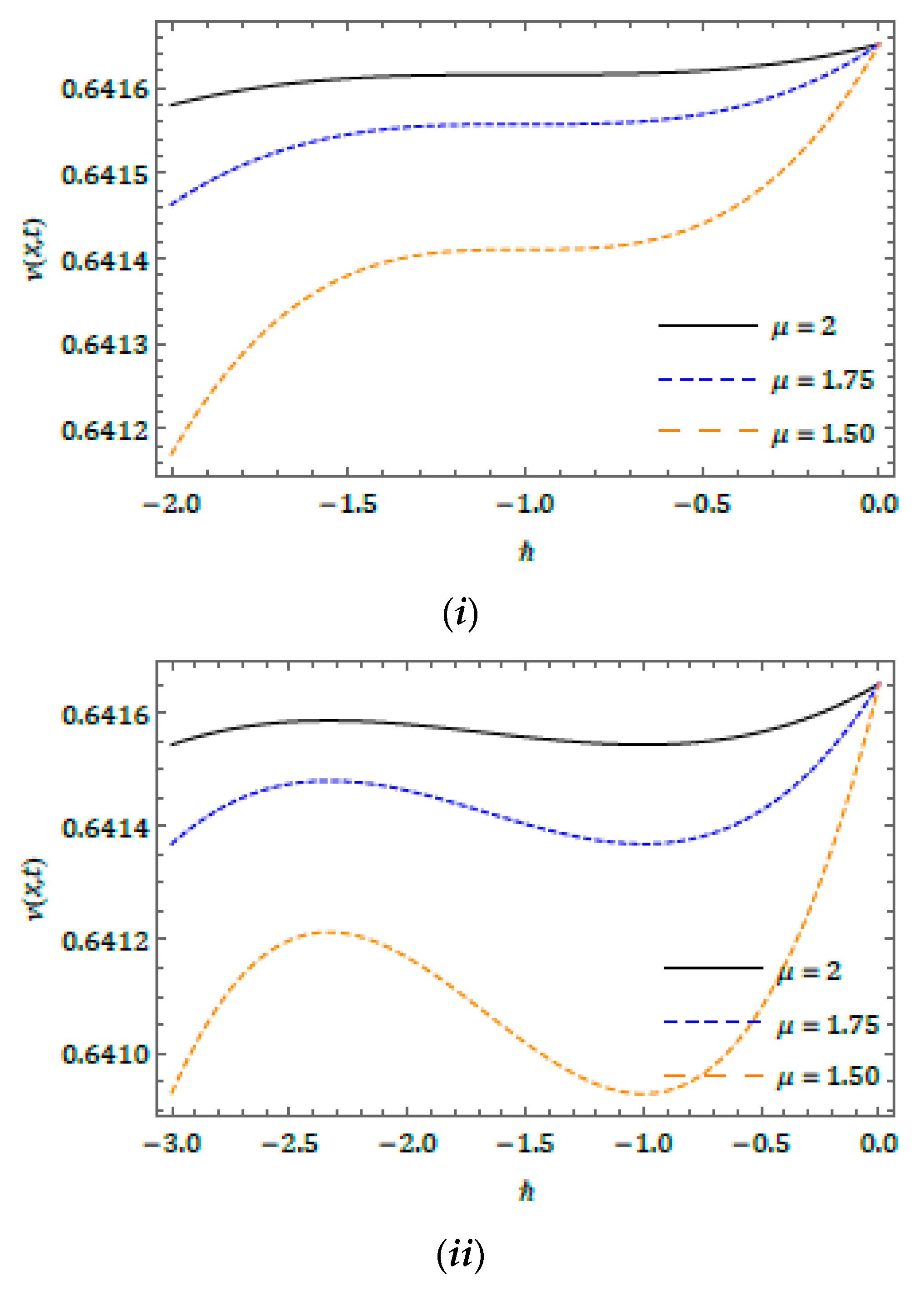
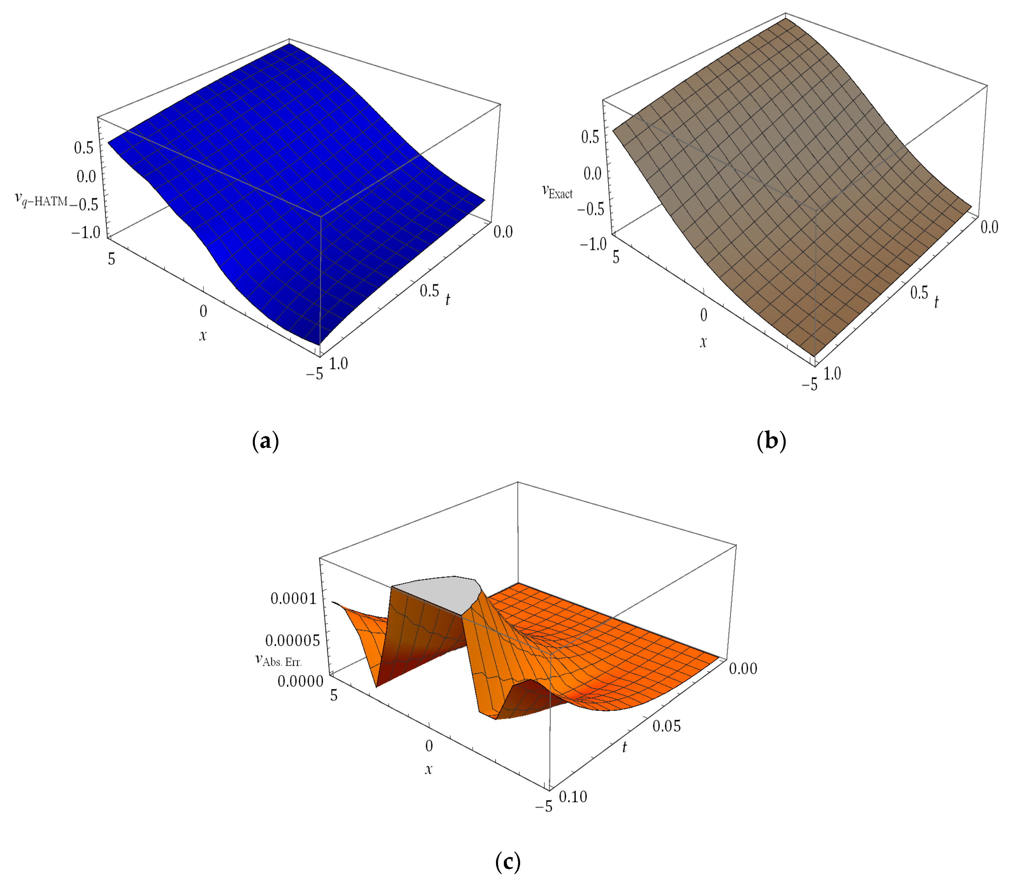
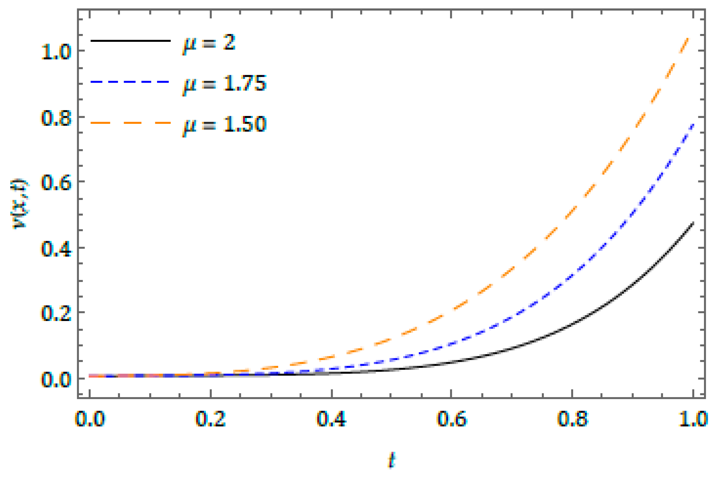
Here, we have demonstrated the numerical simulations of the Phi-four equation having fractional-order by using -HATM. The fourth order solution (i.e., up to ) we consider to illustrate the behavior of the obtained solution in terms of plots and tables. In Table 1 and Table 2, the numerical studies have been conducted to ensure the exactness of the projected algorithm, and further from the tables, it is confirmed that the considered model conspicuously depends on the time. The surfaces of the -HATM solution, exact solution and absolute error are captured in Figure 1 for the FPF equation considered in Example 1. To show the projected problem remarkably depends on arbitrary order and the response of -HATM solution for different , the plots have been drowned and are cited in Figure 2 and Figure 5 for Examples 1 and 2., respectively. Similarly, nature obtained and exact solutions in association with absolute error for Example 2, are presented in Figure 4. The -curves have been drowned to analyze the behavior of the achieved solution related homotopy parameter with different for both examples and have been respectively captured in Figure 3 and Figure 6. These curves can help us to adjust and regulate the region of convergence for the -HATM solution. For unsuitable , the -HATM solution swiftly converges to exact solution. The demonstrated plots help us to better understand the nature of the fractional Phi-four equation when temporal-spatial variables vary in comparison with arbitrary order.
7. Conclusions
In the present framework, -HATM has been employed to find the numerical solutions for the fractional Phi-four equation. With the help of Banach’s fixed point theory, the convergence analysis projecting the nonlinear problem has been presented. To present the efficiency as well as the applicability of the projected algorithm, we have considered two distinct cases. The present study confirms that the projected nonlinear problem is remarkable with the time instant as well as the time history and these can be effectively exemplified by employing the concept of fractional calculus. The governing model plays a vibrant role while analyzing many physical phenomena, and thus, for future work, this can be examined by using recently proposed and nurtured effective and accurate methods [87,88]. With the help of the obtained results, we can capture more interesting consequences. Finally, it has been observed that the considered scheme is highly effective, more accurate and extremely methodical, and this can be employed to exemplify the various classes of nonlinear models that exist in science and technology. The results obtained demonstrate that the considered method is more effective and easy to employ to scrutinize the behaviors of fractional differential equations with multi-dimensions arising in associated areas of science and technology.
Author Contributions
Conceptualization, D.G.P.; writing—original draft preparation, P.V.; supervision, W.G. and H.M.B., G.Y. All authors have read and agreed to the published version of the manuscript.
Funding
This research received no external funding.
Acknowledgments
We thank the helpful and important suggestions of the editors and reviewers.
Conflicts of Interest
The authors declare no conflict of interest.
References
- Liouville, J. Memoire surquelques questions de geometrieet de mecanique, etsurun nouveau genre de calcul pour resoudrecesquestions. J. Ecole Polytech. 1832, 13, 1–69. [Google Scholar]
- Riemann, G.F.B. Versuch Einer Allgemeinen Aufassung der Integration und Diferentiation; Gesammelte Mathematische Werke: Leipzig, Germany, 1896. [Google Scholar]
- Caputo, M. Elasticita e Dissipazione; Zanichelli: Bologna, Italy, 1969. [Google Scholar]
- Miller, K.S.; Ross, B. An Introduction to Fractional Calculus and Fractional Differential Equations; Wiley: New York, NY, USA, 1993. [Google Scholar]
- Podlubny, I. Fractional Differential Equations; Academic Press: New York, NY, USA, 1999. [Google Scholar]
- Kilbas, A.A.; Srivastava, H.M.; Trujillo, J.J. Theory and Applications of Fractional Differential Equations; Elsevier: Amsterdam, The Netherlands, 2006. [Google Scholar]
- Cruz-Duarte, J.M.; Garcia, J.R.; Correa-Cely, C.R.; Perez, A.G.; Avina-Cervantes, J.G. A closed form expression for the Gaussian-based Caputo-Fabrizio fractional derivative for signal processing applications. Commun. Nonlinear Sci. Numer. Simul. 2018, 61, 138–148. [Google Scholar] [CrossRef]
- Esen, A.; Sulaiman, T.A.; Bulut, H.; Baskonus, H.M. Optical solitons and other solutions to the conformable space–time fractional Fokas–Lenells equation. Optik 2018, 167, 150–156. [Google Scholar] [CrossRef]
- Sweilam, N.H.; Hasan, M.M.A.; Baleanu, D. New studies for general fractional financial models of awareness and trial advertising decisions. Chaos Solitons Fractals 2017, 104, 772–784. [Google Scholar] [CrossRef]
- Baleanu, D.; Wu, G.C.; Zeng, S.D. Chaos analysis and asymptotic stability of generalized Caputo fractional differential equations. Chaos Solitons Fractals 2017, 102, 99–105. [Google Scholar] [CrossRef]
- Veeresha, P.; Prakasha, D.G.; Baskonus, H.M. New numerical surfaces to the mathematical model of cancer chemotherapy effect in Caputo fractional derivatives. Chaos 2019, 29. [Google Scholar] [CrossRef]
- Atangana, A. Fractional discretization: The African’s tortoise walk. Chaos Solitons Fractals 2020, 130, 109399. [Google Scholar] [CrossRef]
- Singh, J.; Kumar, D.; Hammouch, Z.; Atangana, A. A fractional epidemiological model for computer viruses pertaining to a new fractional derivative. Appl. Math. Comput. 2018, 316, 504–515. [Google Scholar]
- Kolade, O.M.; Hammouch, Z. Mathematical modeling and analysis of two-variable system with noninteger-order derivative. Chaos 2019, 29, 013145. [Google Scholar]
- Khan, M.A.; Hammouch, Z.; Baleanu, D. Modeling the dynamics of hepatitis E via the Caputo–Fabrizio derivative. Math. Model. Nat. Phenom. 2019, 14, 311. [Google Scholar] [CrossRef]
- Prakash, A.; Veeresha, P.; Prakasha, D.G.; Goyal, M. A homotopy technique for fractional order multi-dimensional telegraph equation via Laplace transform. Eur. Phys. J. Plus 2019, 134, 1–18. [Google Scholar] [CrossRef]
- Cattani, C.; Srivastava, H.M.; Yang, X.J. Fractional Dynamics; De Gruyter: Berlin, Germany, 2019; pp. 1–5. [Google Scholar]
- Zhang, Y.; Cattani, C.; Yang, X.J. Local fractional homotopy perturbation method for solving non-homogeneous heat conduction equations in fractal domains. Entropy 2015, 17, 6753–6764. [Google Scholar] [CrossRef] [Green Version]
- Veeresha, P.; Prakasha, D.G.; Baskonus, H.M. Solving smoking epidemic model of fractional order using a modified homotopy analysis transform method. Math. Sci. 2019, 13, 115–128. [Google Scholar] [CrossRef] [Green Version]
- Atangana, A.; Baleanu, D. New fractional derivatives with non-local and non-singular kernel theory and application to heat transfer model. Therm. Sci. 2016, 20, 763–769. [Google Scholar] [CrossRef] [Green Version]
- Seadawy, A.R. Fractional solitary wave solutions of the nonlinear higher-order extended KdV equation in a stratified shear flow: Part I. Comp. Math. Appl. 2015, 70, 345–352. [Google Scholar] [CrossRef]
- Atangana, A.; Alkahtani, B.T. Analysis of the Keller-Segel model with a fractional derivative without singular kernel. Entropy 2015, 17, 4439–4453. [Google Scholar]
- Kaya, D.; Gulbahar, S.; Yokus, A.; Gulbahar, M. Solutions of the fractional combined kdv–mkdv equation with collocation method using radial basis function and their geometrical obstructions. Adv. Differ. Equ. 2018, 77, 2018. [Google Scholar] [CrossRef]
- Prakash, A.; Prakash, D.G.; Veeresha, P. A reliable algorithm for time-fractional Navier-Stokes equations via Laplace transforms. Nonlinear Eng. 2019, 8, 695–701. [Google Scholar] [CrossRef]
- Kumar, D.; Singh, J.; Baleanu, D. Analysis of regularized long-wave equation associated with a new fractional operator with Mittag-Leffler type kernel. Physica A 2018, 492, 155–167. [Google Scholar] [CrossRef]
- Brzeziński, D.W. Review of numerical methods for NumILPT with computational accuracy assessment for fractional calculus. Appl. Math. Nonlinear Sci. 2018, 3, 487–502. [Google Scholar] [CrossRef] [Green Version]
- Youssef, I.K.; Dewaik, M.H. Solving Poisson’s Equations with fractional order using Haarwavelet. Appl. Math. Nonlinear Sci. 2017, 2, 271–284. [Google Scholar] [CrossRef] [Green Version]
- Singh, J.; Kumar, D.; Baleanu, D. New aspects of fractional Biswas-Milovic model with Mittag-Leffler law. Math. Modelling Nat. Phenomena 2019, 14, 303–310. [Google Scholar] [CrossRef] [Green Version]
- Cattani, C.; Ciancio. On the fractal distribution of primes and prime-indexed primes by the binary image analysis. Phys. A 2016, 460, 222–229. [Google Scholar] [CrossRef]
- Cattani, C. A review on Harmonic Wavelets and their fractional extension. J. Adv. Eng. Comput. 2018, 2, 224–238. [Google Scholar] [CrossRef] [Green Version]
- Veeresha, P.; Prakasha, D.G.; Baskonus, H.M. An efficient technique for a fractional-order system of equations describing the unsteady flow of a polytropic gas. Pramana 2019, 93, 75. [Google Scholar] [CrossRef]
- Prakasha, D.G.; Veeresha, P.; Singh, J. Fractional approach for equation describing the water transport in unsaturated porous media with Mittag-Leffler kernel. Front. Phys. 2019, 7, 193. [Google Scholar] [CrossRef] [Green Version]
- Baleanu, D.; Jajarmi, A.; Sajjadi, S.S.; Mozyrska, D. A new fractional model and optimal control of a tumor-immune surveillance with non-singular derivative operator. Chaos 2019, 29, 083127. [Google Scholar] [CrossRef]
- Jajarmi, A.; Arshad, S.; Baleanu, D. A new fractional modelling and control strategy for the outbreak of dengue fever. Phys. A 2019, 535. [Google Scholar] [CrossRef]
- Jajarmi, A.; Ghanbari, B.; Baleanu, D. A new and efficient numerical method for the fractional modeling and optimal control of diabetes and tuberculosis co-existence. Chaos 2019, 29. [Google Scholar] [CrossRef]
- Jajarmi, A.; Baleanu, D.; Sajjadi, S.S.; Asad, J.H. A new feature of the fractional Euler–Lagrange equations for a coupled oscillator using a nonsingular operator approach. Front. Phys. 2019, 7. [Google Scholar] [CrossRef] [Green Version]
- Baleanu, D.; Asad, J.H.; Jajarmi, A. New aspects of the motion of a particle in a circular cavity. Proc. Rom. Acad. Ser. A 2018, 19, 361–367. [Google Scholar]
- Veeresha, P.; Prakasha, D.G. Solution for fractional Zakharov-Kuznetsov equations by using two reliable techniques. Chin. J. Phys. 2019, 60, 313–330. [Google Scholar] [CrossRef]
- Baleanu, D.; Sajjadi, S.S.; Jajarmi, A.; Asad, J.H. New features of the fractional Euler-Lagrange equations for a physical system within non-singular derivative operator. Eur. Phys. J. Plus 2019, 134. [Google Scholar] [CrossRef]
- Sulaiman, T.A.; Bulut, H.; Baskonus, H.M. Optical solitons to the fractional perturbed NLSE in nano-fibers. Discret. Contin. Dyn. Syst. Ser. S 2019, 13, 925–936. [Google Scholar]
- Dashen, R.F.; Hasslacher, B.; Neveu, A. Particle spectrum in model field theories from semi-classical functional integral technique. Phys. Rev. D. 1975, 11, 3424–3450. [Google Scholar] [CrossRef]
- Wazwaz, A.M. Generalized forms of the phi-four equation with compactons, solitons and periodic solutions. Math. Comput. Simul. 2005, 69, 580–588. [Google Scholar] [CrossRef]
- Liao, S.J. The Proposed Homotopy Analysis Technique for the Solution of Nonlinear Problems. Ph.D. Thesis, Shanghai Jiao Tong University, Shanghai, China, 1992. [Google Scholar]
- Liao, S.J. Homotopy analysis method and its applications in mathematics. J. Basic Sci. Eng. 1997, 5, 111–125. [Google Scholar]
- Singh, J.; Kumar, D.; Swroop, R. Numerical solution of time- and space-fractional coupled Burgers’ equations via homotopy algorithm. Alex. Eng. J. 2016, 55, 1753–1763. [Google Scholar] [CrossRef] [Green Version]
- Srivastava, H.M.; Kumar, D.; Singh, J. An efficient analytical technique for fractional model of vibration equation. Appl. Math. Model. 2017, 45, 192–204. [Google Scholar] [CrossRef]
- Kumar, D.; Singh, J.; Baleanu, D. A New Numerical Algorithm for Fractional Fitzhugh-Nagumo Equation Arising in Transmission of Nerve Impulses. Nonlinear Dyn. 2018, 91, 307–317. [Google Scholar] [CrossRef]
- Singh, J.; Secer, A.; Swroop, R.; Kumar, D. A reliable analytical approach for a fractional model of advection-dispersion equation. Nonlinear Eng. 2019, 9, 107–116. [Google Scholar] [CrossRef]
- Veeresha, P.; Prakasha, D.G.; Baskonus, H.M. Novel simulations to the time-fractional Fisher’s equation. Math. Sci. 2019, 13, 33–42. [Google Scholar] [CrossRef]
- Singh, J.; Kumar, D.; Swroop, R.; Kumar, S. An efficient computational approach for time-fractional Rosenau-Hyman equation. Neural Comput. Appl. 2018, 30, 3063–3070. [Google Scholar] [CrossRef]
- Prakasha, D.G.; Veeresha, P.; Baskonus, H.M. Two novel computational techniques for fractional Gardner and Cahn-Hilliard equations. Comput. Math. Methods 2019, 1, e1021. [Google Scholar] [CrossRef] [Green Version]
- Veeresha, P.; Prakasha, D.G.; Kumar, D. An efficient technique for nonlinear time-fractional Klein-Fock-Gordon equation. Appl. Math. Comput. 2020, 364, 124637. [Google Scholar] [CrossRef]
- Kumar, D.; Agarwal, R.P.; Singh, J. A modified numerical scheme and convergence analysis for fractional model of Lienard’s equation. J. Comput. Appl. Math. 2018, 399, 405–413. [Google Scholar] [CrossRef]
- Veeresha, P.; Prakasha, D.G.; Baleanu, D. An efficient numerical technique for the nonlinear fractional Kolmogorov-Petrovskii-Piskunov equation. Mathematics 2019, 7, 365. [Google Scholar] [CrossRef] [Green Version]
- Prakash, A.; Veeresha, P.; Prakasha, D.G.; Goyal, M. A new efficient technique for solving fractional coupled Navier–Stokes equations using q-homotopy analysis transform method. Pramana 2019, 93, 6. [Google Scholar] [CrossRef]
- Veeresha, P.; Prakasha, D.G. Solution for fractional generalized Zakharov equations with Mittag-Leffler function. Results Eng. 2020, 5, 100085. [Google Scholar] [CrossRef]
- Rezazadeh, H.; Tariq, H.; Eslami, M.; Mirzazadeh, M.; Zhou, Q. New exact solutions of nonlinear conformable time-fractional Phi-4 equation. Chin. J. Phys. 2018, 56, 2805–2816. [Google Scholar] [CrossRef]
- Bhrawy, A.H.; Assas, L.M.; Alghamdi, M.A. An efficient spectral collocation algorithm for nonlinear Phi-four equations. Bound. Value Probl. 2013, 2013, 87. [Google Scholar] [CrossRef] [Green Version]
- Tariq, H.; Akram, G. New approach for exact solutions of time fractional Cahn–Allen equation and time fractional Phi-4 equation. Phys. A 2017, 473, 352–362. [Google Scholar] [CrossRef]
- Zahra, W.K. Trigonometric B-Spline collocation method for solving PHI-four and Allen–Cahn equations. Mediterr. J. Math. 2017, 14, 122. [Google Scholar] [CrossRef]
- Gao, W.; Ghanbari, B.; Baskonus, H.M. New numerical simulations for some real world problems with Atangana-Baleanu fractional derivative. Chaos Solitons Fractals 2019, 128, 34–43. [Google Scholar] [CrossRef]
- Mahmud, F.; Samsuzzoh, M.; Akbar, M.A. The generalized Kudryashov method to obtain exact traveling wave solutions of the PHI-four equation and the Fisher equation. Results Phys. 2017, 7, 4296–4302. [Google Scholar] [CrossRef]
- Gao, W.; Partohaghighi, M.; Baskonus, H.M.; Ghavi, S. Regarding the Group preserving scheme and method of line to the Numerical Simulations of Klein-Gordon Model. Results Phys. 2019, 15, 102555. [Google Scholar] [CrossRef]
- Gao, W.; Veeresha, P.; Prakasha, D.G.; Baskonus, H.M.; Yel, G. A powerful approach for fractional Drinfeld–Sokolov–Wilson equation with Mittag-Leffler law. Alex. Eng. J. 2019. [Google Scholar] [CrossRef]
- Gao, W.; Ismael, H.F.; Mohammed, S.A.; Baskonus, H.M.; Bulut, H. Complex and real optical soliton properties of the paraxial nonlinear Schrödinger equation in Kerr media with M-fractional. Front. Phys. 2019. [Google Scholar] [CrossRef] [Green Version]
- Yokus, A.; Gulbahar, S. Numerical Solutions with Linearization Techniques of the Fractional Harry Dym Equation. Appl. Math. Nonlinear Sci. 2019, 4, 35–42. [Google Scholar] [CrossRef] [Green Version]
- Gao, W.; Yel, G.; Baskonus, H.M.; Cattani, C. Complex Solitons in the Conformable (2+1)-dimensional Ablowitz-Kaup-Newell-Segur Equation. AIMS Math. 2020, 5, 507–521. [Google Scholar] [CrossRef]
- Al-Ghafri, K.S.; Rezazadeh, H. Solitons and other solutions of (3 + 1)-dimensional space–time fractional modified KdV–Zakharov–Kuznetsov equation. Appl. Math. Nonlinear Sci. 2019, 4, 289–304. [Google Scholar] [CrossRef] [Green Version]
- Ciancio, A.; Quartarone, A. A hybrid model for tumor-immune competition. UPB Sci. Bull. Ser. A 2013, 75, 125–136. [Google Scholar]
- Yel, G.; Baskonus, H.M. Solitons in Conformable Time-Fractional Wu-Zhang System Arising in Coastal Design. Pramana 2019, 93, 57. [Google Scholar] [CrossRef]
- Yang, X.J. New rheological problems involving general fractional derivatives with nonsingular power-law kernels. Proc. Rom. Acad. Ser. A Math. Phys. Tech. Sci. Inf. Sci. 2018, 19, 45–52. [Google Scholar]
- Baskonus, H.M. Complex Surfaces to the Fractional (2+1)-dimensional Boussinesq Dynamical Model with Local M-derivative. Eur. Phys. J. Plus 2019, 134, 322. [Google Scholar] [CrossRef]
- Lemkeddem, M.; Hammouch, Z.; Guerbati, K.; Benchohra, M. Impulsive partial functional fractional differential equations with non-local conditions. Nonlinear Stud. 2019, 10, 303–321. [Google Scholar]
- Ciancio, A. Analysis of time series with wavelets. Int. J. Wavelets Multiresolut. Inf. Process. 2007, 5, 241–256. [Google Scholar] [CrossRef]
- Yang, X.J. New general fractional-order rheological models with kernels of Mittag-Leffler functions. Rom. Rep. Phys. 2017, 69, 118. [Google Scholar]
- Tellab, B.; Haouam, K. Solvability of semilinear fractional differential equations with nonlocal and integral boundary conditions. Nonlinear Stud. 2019, 10, 341–356. [Google Scholar]
- Velioglu, Z. Soluble Product of Parafree Lie algebras and Its residual Properties. Appl. Math. Nonlinear Sci. 2019, 4, 1–5. [Google Scholar] [CrossRef]
- Kocak, Z.F.; Bulut, H.; Yel, G. The solution of fractional wave equation by using modified trial equation method and homotopy analysis method. AIP Conference Proceedings 2014, 1637, 504–512. [Google Scholar]
- Rani, D.; Mishra, V. Solving linear fractional order differential equations by Chebyshev polynomials based numerical inverse Laplace transform. Nonlinear Stud. 2019, 10, 781–791. [Google Scholar]
- Klimek, M.; Lupa, M. Reflection Symmetry in Fractional Calculus–Properties and Applications. In Advances in the Theory and Applications of Non-integer Order Systems; Springer: Heidelberg, Germany, 2013; pp. 201–211. [Google Scholar]
- Odibat, Z.M.; Shawagfeh, N.T. Generalized Taylor’s formula. Appl. Math. Comput. 2007, 186, 286–293. [Google Scholar] [CrossRef]
- Argyros, I.K. Convergence and Applications of Newton-Type Iterations; Springer: New York, NY, USA, 2008. [Google Scholar]
- Magrenan, A.A. A new tool to study real dynamics: The convergence plane. Appl. Math. Comput. 2014, 248, 215–224. [Google Scholar] [CrossRef] [Green Version]
- Alquran, M.; Jaradat, H.M.; Syam, M.I. Analytical solution of the time-fractional Phi-4 equation by using modified residual power series method. Nonlinear Dyn. 2017, 90, 2525–2529. [Google Scholar] [CrossRef]
- Zhou, H.; Shen, J. Bifurcations of travelling wave solutions for modified nonlinear dispersive phi-four equation. Appl. Math. Comput. 2010, 217, 1584–1597. [Google Scholar] [CrossRef]
- Deng, X.; Zhao, M.; Li, X. Travelling wave solutions for a nonlinear variant of the PHI-four equation. Math. Comput. Model. 2009, 49, 617–622. [Google Scholar] [CrossRef]
- Veeresha, P.; Prakasha, D.G.; Singh, J. Solution for fractional forced KdV equation using fractional natural decomposition method. AIMS Math. 2019, 5, 798–810. [Google Scholar] [CrossRef]
- Veeresha, P.; Prakasha, D.G. An efficient technique for two-dimensional fractional order biological population model. Int. J. Model. Simul. Sci. Comput. 2020. [Google Scholar] [CrossRef]
Figure 1.
3D graphs of Obtained solution, Exact solution, Absolute error for Example 1 at and .

Figure 2.
2D graph of -homotopy analysis transform method ( -HATM) solution at and with distinct for Example 1.
Figure 2.
2D graph of -homotopy analysis transform method ( -HATM) solution at and with distinct for Example 1.
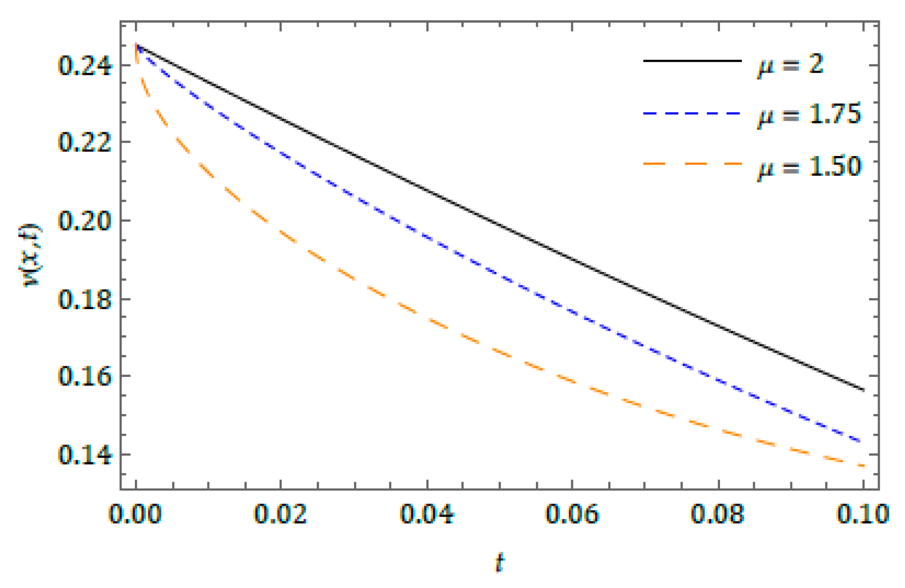
Figure 3.
2D graphs of -curves for of Example 1 at with different with and .
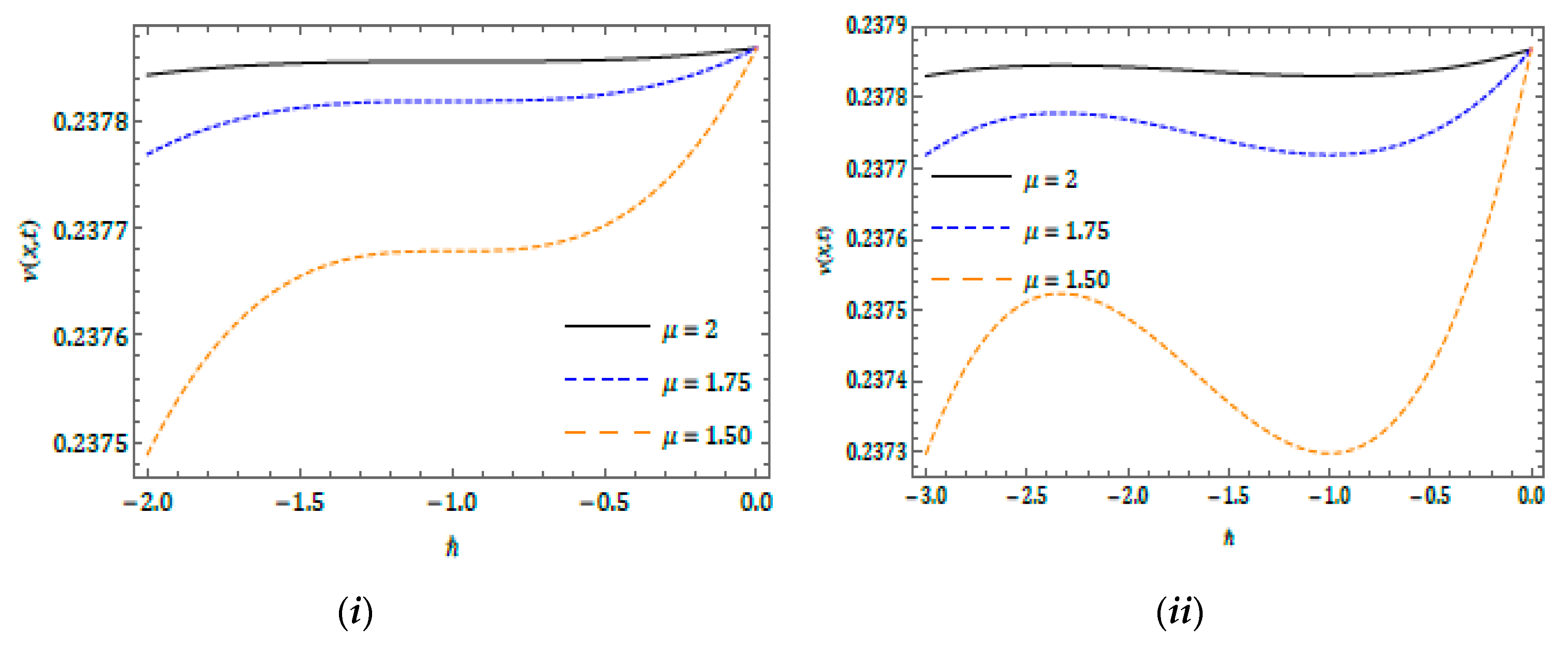
Figure 4.
3Dsurfaces of -HATM solution, Exact solution, Absolute error for Example2 at and .
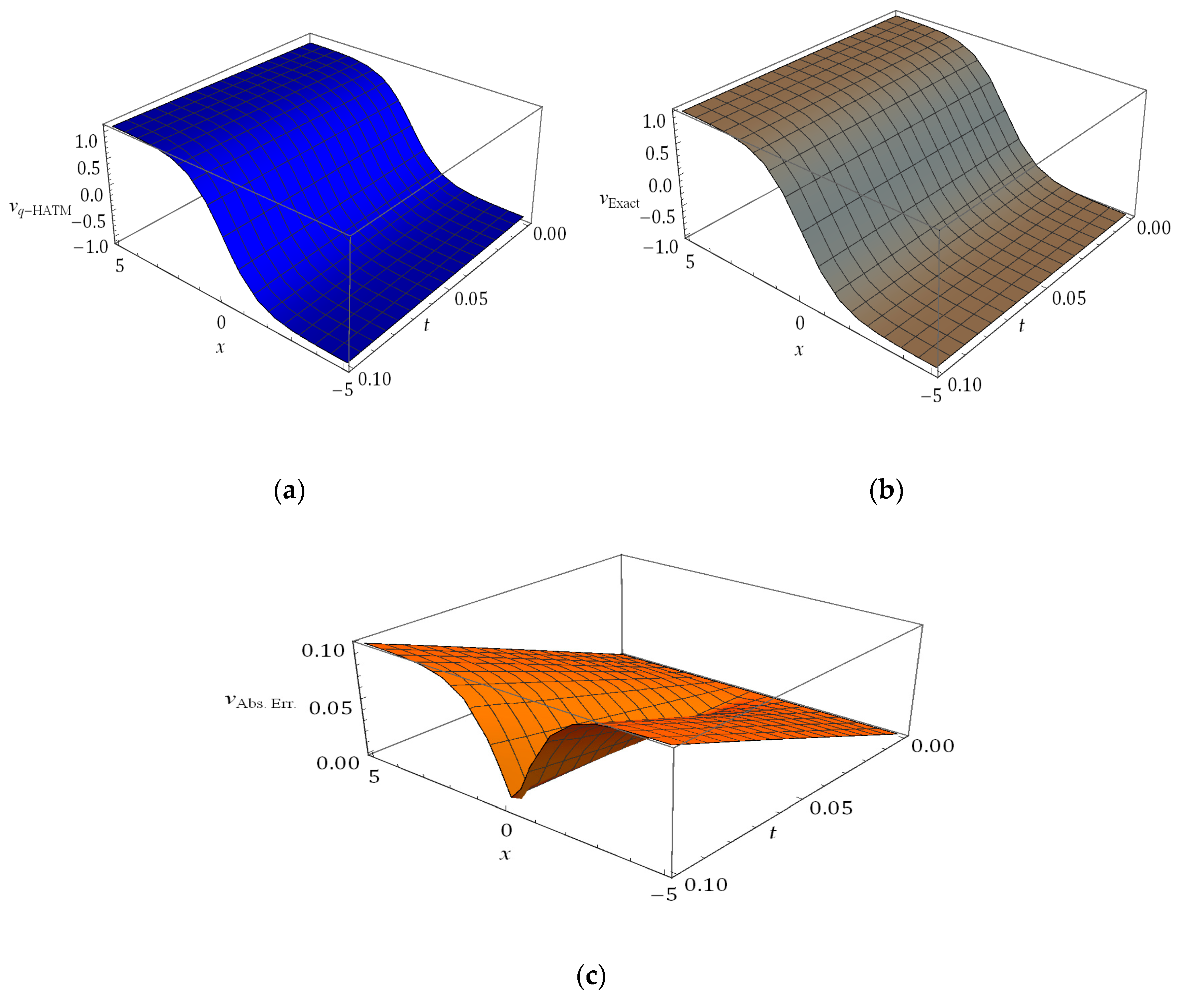
Figure 5.
2D graph of -HATM solution at and with different for Example2.

Figure 6.
2D graphs of for of Example2 at with distinct with and .

Table 1.
Numerical simulation conducted for FPF equation defined in Example1 with different and at and .
Table 1.
Numerical simulation conducted for FPF equation defined in Example1 with different and at and .
Table 2.
Numerical simulation conducted for fractional Phi-four (FPF) equation defined in Example2 with different and at and .
Table 2.
Numerical simulation conducted for fractional Phi-four (FPF) equation defined in Example2 with different and at and .
© 2020 by the authors. Licensee MDPI, Basel, Switzerland. This article is an open access article distributed under the terms and conditions of the Creative Commons Attribution (CC BY) license (http://creativecommons.org/licenses/by/4.0/).
Share and Cite
MDPI and ACS Style
Gao, W.; Veeresha, P.; Prakasha, D.G.; Baskonus, H.M.; Yel, G. New Numerical Results for the Time-Fractional Phi-Four Equation Using a Novel Analytical Approach. Symmetry 2020, 12, 478. https://doi.org/10.3390/sym12030478
AMA Style
Gao W, Veeresha P, Prakasha DG, Baskonus HM, Yel G. New Numerical Results for the Time-Fractional Phi-Four Equation Using a Novel Analytical Approach. Symmetry. 2020; 12(3):478. https://doi.org/10.3390/sym12030478
Chicago/Turabian StyleGao, Wei, Pundikala Veeresha, Doddabhadrappla Gowda Prakasha, Haci Mehmet Baskonus, and Gulnur Yel. 2020. "New Numerical Results for the Time-Fractional Phi-Four Equation Using a Novel Analytical Approach" Symmetry 12, no. 3: 478. https://doi.org/10.3390/sym12030478
Note that from the first issue of 2016, this journal uses article numbers instead of page numbers. See further details here.