Stochastic Empty Container Repositioning Problem with CO2 Emission Considerations for an Intermodal Transportation System

School of Traffic and Transportation, Beijing Jiaotong University, Beijing 100044, China
*
Author to whom correspondence should be addressed.
Sustainability 2018, 10(11), 4211; https://doi.org/10.3390/su10114211
Submission received: 19 October 2018
/
Revised: 11 November 2018
/
Accepted: 13 November 2018
/
Published: 15 November 2018
(This article belongs to the Section Sustainable Transportation)
Abstract
:As one of main challenge for carriers, empty container repositioning is subject to various uncertain factors in practice, which causes more operation costs. At the same time, the movements of empty containers can result in air pollution because of the CO2 emission, which has a negative impact on sustainable development. To incorporate environmental and stochastic characteristics of container shipping, in this paper, an empty container repositioning problem, taking into account CO2 emission, stochastic demand, and supply, is introduced in a sea–rail intermodal transportation system. This problem is formulated as a chance-constrained nonlinear integer programming model minimising the expected value of total weighted cost. A sample average approximation method is applied to convert this model into its deterministic equivalents, which is then solved by the proposed two-phase tabu search algorithm. A numerical example is studied to conclude that the stochastic demand and supply lead to more repositioning and CO2 emission-related cost. Total cost, inventory cost, and leasing cost increase with the variabilities of uncertain parameters. We also found that the total cost and other component costs are strongly dependent on the weights of repositioning cost and CO2 emission-related cost. Additionally, the sensitivity analysis is conducted on unit leasing cost.
1. Introduction
Due to the overwhelming growth of international trade in recent years, international freight transportation develops rapidly. Compared to unimodal freight transportation (e.g., railway, road, and maritime transportation), intermodal freight transportation is more competitive and advantageous with respect to security, flexibility, and productivity [1]. A significant amount of containers being transshipped are empty. As a result, intermodal freight transportation has been playing a more and more important role in global freight transportation [2]. Owing to different economic needs in different regions, the volumes of import and export trade in many regions are also quite different, which leads to the imbalance of global trade. For instance, the container flow from Eastern Asia to North America reaches a volume of 17.9 million TEUs, while the volume of the opposite direction (i.e., from North to Eastern Asia) was only 8.2 million TEUs, in 2017 [3]. Consequently, intermodal freight industries have to reposition empty containers, from the regions with empty container accumulation to the regions with empty container shortage. However, in practice, the surplus empty containers sometimes are not sufficient to fulfil the customer’s demand. Thus, additional empty containers need to be leased from leasing companies, which is a more responsive way compared with repositioning. As a result, intermodal freight industries should make a highly efficient operation plan with minimal expenditure, which allocates surplus empty containers from supply regions to demand regions, and determines the number of leased empty containers in demand regions.
In addition to minimising the operational cost, traffic pollution should be considered [4]. Recently, transportation growth has become one of main factors contributing to the increase of CO2 emissions [5]. Take maritime transportation for example, in 2012, total shipping CO2 emissions were estimated at 938 million tons accounting for 2.6% of global CO2 emissions. Among this, international shipping emission was approximately 796 million tons CO2 [6]. Therefore, both operation cost and CO2 emissions should be considered simultaneously in the process of repositioning empty containers.
This paper focuses on the empty container repositioning problem (ECRP), with the consideration of leasing decisions and CO2 emissions in an intermodal sea–rail network. The ECRP is defined as to determine how many empty containers should be repositioned, which route should be used to transport empty containers, as well as where and how many empty containers should be leased in order to satisfy the demands.
As an intrinsic issue of container management and intermodal transportation, ECRP has received more attention in recent years (e.g., [7,8,9]). As a consequence, there is substantial literature on ECRP. Some of the studies provide concise and precise updates on the latest progress made in the area of ECRP research from different perspectives (e.g., [10,11]). Specifically, Braekers et al. [10] conducted a comprehensive overview of ECRP at a regional level from three different planning levels, i.e., strategic level, tactical level, and operational level. Song and Dong [11] provided a detailed literature review focusing on the ECRP models for different transportation networks, and sorted them into two categories: network flow models and inventory control-based models. Table 1 lists the key references on ECRP, in terms of transportation model, stochasticity, and CO2 emissions.
Generally, the literature could be classified into two categories: deterministic ECRP and stochastic ECRP. For deterministic ECRP, in the pioneer study of Florez [12], a model based on a dynamic transshipment network was established for optimising ECRP, which considered repositioning and leasing empty containers simultaneously. Crainic and Delorme [13] described ECRP as a multicommodity location–allocation problem with balance requirements, and employed a dual-ascent solution approach to solve it. Song and Carter [15] considered ECRP from the perspective of ocean carriers, identified critical factors affecting ECRP, and investigated the influence of route coordination and container sharing. Moon et al. [16] developed a mixed integer programming model for ECRP, incorporating the policies of leasing and purchasing containers to minimise total cost. A hybrid genetic algorithm was employed to solve the proposed model.
Different from the literature above, some papers allow for ECRP with other decision-making problems, e.g., cargo routing problem, service network design problem, and ship deployment problem. For instance, Brouer et al. [17] addressed the cargo routing problem and ECRP simultaneously, and formulated it as a multi-commodity flow problem with interbalancing constraints, which was solved by the delayed column generation algorithm. The problem was further studied by Song and Dong [19] on a maritime transportation network with multiple service routes, deployed vessels, and regular voyages. Regarding service network design problem, Shintani et al. [14] studied the ECRP combined with a container liner service network design, which was formulated as a two-stage problem solved by a heuristic based on genetic algorithm. This problem was later investigated by Meng and Wang [18], who proposed a mixed integer linear programming model to formulate this problem. In their study, the concept of segment was firstly introduced to facilitate the problem formulation. A realistic case of Asia–Europe–Oceania shipping was carried out to demonstrate the proposed model, and concluded that the total operation cost could be reduced significantly by considering empty container repositioning. The ECRP raised by these two papers is limited to global ocean shipping. By contrast, An et al. [21] presented the service network design for inland water liner transportation with ECRP. By incorporating the specific features of inland water transportation, a nonlinear mixed integer programming model was constructed, and subsequently solved by a hybrid algorithm integrating genetic algorithm and integer programming method. Furthermore, Song and Dong [20] proposed a three-stage solution methodology, where the first, second, and third stage were used to deal with the service network design problem, ECRP, and ship deployment problem, respectively.
Compared with the literature about unimodal ECRP, some studies are concerned with the ECRP in an intermodal transportation system. Specifically, Choong et al. [35] analysed the effect of planning horizon length on mode selection of ECRP for intermodal transportation network, and indicated that the slower and cheaper transportation modes are more encouraged under the condition that the planning horizon is long enough. Meng et al. [36] developed a linear mixed integer programming model for intermodal liner service network design, which accounted for laden container routing, ECRP, and ship route selection. A combination of intermodal service network design problem and ECRP was studied by Braekers et al. [37] in a barge hinterland system, and discussed from different perspectives, i.e., the perspective of barge operators and the perspective of shipping lines. In addition to quantitative analysis on ECRP, Kolar et al. [38] described a research agenda of ECRP based on a qualitative analysis by conducting interviews with representatives of ocean carriers, and indicated some insightful findings.
All the literature mentioned above is studied under deterministic circumstances. However, generally, empty container repositioning is subjected to various stochastic factors in practice. For instance, the number of empty containers available cannot be forecasted precisely, because of stochastic demand and supply. For empty container demand, it is difficult to obtain exact future volume, due to a high dynamic environment and low precision forecast [2]. Similarly, the accurate future volume of empty container supply is also hard to estimate, due to the uncertain returning time of containers from customers [22]. Hence, both demand and supply should be described as uncertain parameters when addressing ECRP. To incorporate the stochastic nature of empty container repositioning, many efforts have been made to explore stochastic ECRP models (e.g., [17,18,19,28,31,32,33,34]). Crainic et al. [23] focused on the ECRP that involved stochastic demand and supply modelled as random variables in the context of the land transportation of international maritime shipping. Moreover, Li et al. [24] addressed the ECRP in one port, where the amounts of import and export containers were treated as independent and identically distributed variables. They extended the results to the long-run average case and the infinite-horizon problem with a discounted factor. This problem was further generalized by Li et al. [25] to take multi-ports into consideration. The allocation plan of empty containers was derived by using a heuristic algorithm with ε-optimal policies. Lam et al. [27] presented a dynamic programming model for stochastic ECRP, and introduced an approximate approach based on temporal difference learning. Song and Zhang [30] constructed a fluid flow model for ECRP concerning stochastic demand, which is simulated as a two-state Markov chain. In order to examine the impact of different stochastic demand patterns on ECRP, Song and Dong [31] analysed the performances under three types of different demand distributions (i.e., normal distribution, uniform distribution, and exponential distribution). Lee et al. [32] focused on the joint container fleet sizing problem, and ECRP with the consideration of stochastic demand based on the feedback mechanism of inventory information, while Dong et al. [33] compared the results of different empty container repositioning policies under uncertain demand.
In addition to stochastic demand and supply, there are some papers concentrating on stochastic capacity. For example, Long et al. [2] set up a two-stage stochastic programming model involving uncertain demand, supply, ship weight capacity, and ship space capacity. Stage one determined the operation plan for repositioning empty containers with deterministic parameters, while stage two adjusted the decisions derived from stage one based on the probability distribution of random variables. Sample average approximation and progressive hedging strategy were applied to solve this model. A two-stage stochastic network model for dynamic ECRP was established by Cheung and Chen [22] in an ocean transportation network, to minimise the expected total cost by taking into account stochastic demand, supply, and capacity. Francesco et al. [29] addressed the ECRP in a maritime transportation system concerning stochastic demand, supply, residual transportation capacity of vessels, and loading and unloading capacity.
Additionally, for unimodal ECRP, Song [26] examined the ECRP from the perspective of the optimal stationary policy in two-terminal shuttle service system with uncertain demand. By exploring the structural characteristics of objective function, a Markov decision process method was used to obtain the results. Song and Dong [28] extended this model to the ECRP in a cyclic route under stochastic and dynamic conditions, which analysed the impact of demand patterns, fleet sizes and, in particular, degrees of uncertainty. For stochastic intermodal ECRP, Dong and Song [39] dealt with the container fleet sizing problem, combined with ECRP involving stochastic demand and inland transportation time, and revealed the relationship between the optimal container fleet size and the inland transportation time. Xie et al. [40] emphasised the coordination and sharing issue of empty container management with uncertain demand and supply between a liner company and a rail company. The optimal delivery policy, and its change with initial inventory state, were investigated under the centralised model, whereas a bilateral buy-back contract was designed in the decentralised model.
Although the literature on ECRP is substantial and extensive, most literature mainly focuses on the operation cost of repositioning empty containers, rather than environmental performance, e.g., CO2 emissions. So far, the research on ECRP with CO2 emissions is still scarce, both practically and theoretically. To the best of our knowledge, only Song and Xu [41], and Bernat et al. [34] studied CO2 emissions whilst repositioning empty containers. Song and Xu [41] provided an operational activity-based method to calculate CO2 emissions in relation to ECRP, and revealed the relationship among CO2 emissions, empty container repositioning policies, and handling capacity. More recently, Bernat et al. [34] presented new periodic review policies integrating CO2 emissions, repair option, street-turns, as well as stochastic parameters. A simulation model with metaheuristic approach was then developed to assess the optimality of these policies.
Empty container repositioning is an extremely important issue in the container shipping industry [11]. A highly efficient repositioning plan can effectively reduce the amount of repositioned and leased empty containers, and shorten the total repositioning distance from the nodes with surplus empty containers to the nodes with deficit empty containers, which leads to a reduction of total repositioning cost for container carriers. However, uncertainty in container shipping may have a negative effect on empty container movements [15], which causes the inefficiency, and even infeasibility, of the current repositioning plan. Thus, a reliable and robust repositioning plan is required to tackle these unpredictable factors in the container transportation system. At the same time, a well-organised repositioning plan can also reduce fuel consumption, traffic congestion, and emissions, due to the decrease of empty container movements. Accordingly, empty container repositioning not only has an economic impact on container carriers, but also an environmental influence on the sustainable development of containerised transportation.
To incorporate environmental and stochastic characteristics of container shipping, this paper proposes a chance-constrained programming model for ECRP in an intermodal transportation system, which allows for, explicitly, CO2 emissions and uncertainty simultaneously. Stochastic demand and supply, in the model, are treated as random variables. The purpose of this paper is to determine how many empty containers should be repositioned, which route should be used to transport empty containers, as well as where and how many empty containers should be leased in order to satisfy the demands, which are referred to as distribution plan, routing plan, and leasing plan, respectively. In addition, we conduct a numerical example to evaluate the results obtained under deterministic and stochastic situations, as well as investigate the impact of model parameters and random variables on the total cost and component costs. The main contributions of this paper are three-fold. First and most significantly, it enriches the literature on ECRP by incorporating CO2 emissions, and stochastic demand and supply. The uncertainty of ECRP facilitates us to construct a chance-constrained programming model, achieving a minimal expected total cost. Second, we use sample average approximation (SAA) to convert this model into its deterministic equivalents, and develop a two-phase tabu search algorithm to solve the associated SAA problem. Third, we examine the effects of unit leasing cost, stochastic demand and supply, as well as weights on costs and CO2 emissions.
The rest of this paper is organised as follows. Section 2 formulates stochastic ECRP with CO2 emissions as a chance-constrained programming model. Section 3 presents a hybrid solution methodology integrating a two-phase tabu search algorithm and SAA method. Section 4 illustrates the computational results. The conclusions and future research directions are given in Section 5.
2. Mathematical Model for Stochastic ECRP with CO2 Emissions
The aim of this section is to present a chance-constrained mixed integer programming model for stochastic ECRP with CO2 emissions, minimising the expected total cost. Section 2.1 introduces notations and assumptions, whilst Section 2.2 describes the mathematical model.
2.1. Notations and Assumptions
Table 2 lists notations to be used in the following sections.
The mathematic model for stochastic empty container repositioning is constructed reliant on the following assumptions.
Assumption 1: Compared with other transportation modes, road transportation is unsuitable and costly for transporting containers over long distance, due to its working hour restrictions for truck drivers, infrastructure deficits, and relatively higher operation costs. In addition, because of the pollution caused by the burning process of fuel, it is not an eco-friendly transportation mode. Therefore, only two transportation modes are taken into account, i.e., railway transportation and maritime transportation. Thus, the intermodal network we discuss in this problem only includes two types of nodes, i.e., railway stations and ports.
Assumption 2: The stochastic demand and supply of empty containers at any railway station and port are independent of time periods. That is, the variabilities of stochastic demand and supply are kept the same during the planning horizon.
Assumption 3: CO2 emission is only incurred by transporting empty containers from the nodes with surplus empty containers to the nodes with deficit empty containers. In other words, it is assumed that leasing empty containers will not contribute to CO2 emission.
Assumption 4: There is no restriction on the amount of leased empty containers at any railway station and port at any time period. When surplus empty containers cannot satisfy the demand, sufficient empty containers are leased to fulfil the shortage in a complementary way. In addition, the leased empty containers are not required to be returned in the planning horizon.
Assumption 5: In order to simplify this model and reduce computational burden, the ECRP in this paper is addressed, regardless of multiple types of containers. Therefore, we only consider the standard containers, i.e., twenty-foot equivalent unit (TEU).
Assumption 6: All empty containers can be used without considering damage, repairs, and discards during the planning horizon. This assumption can be relaxed by adding the percentages of defective empty containers into the model if necessary.
Assumption 7: The scope of this study is limited to the regional intermodal network, including railway hinterland network of ports and the ship routes among these ports. Additionally, the train services are all assumed to be direct, to ensure that inland transportation time is short enough compared with the one time period. Similarly, the travel times of all ship routes are much smaller than one time period. Consequently, we assume that all repositioned empty containers can be transported from their origins to their destinations within one time period.
Assumption 8: All demands of empty containers can be satisfied at each time period by repositioning and leasing empty containers, which is consistent with Assumption 4.
Assumption 9: For the stochastic demands at each railway station and port, they follow different uniform distributions, respectively, with the same variability but different expected values. The stochastic supplies are in the same manner as illustrated in Section 4.2.
2.2. A Chance-Constrained Nonlinear Integer Programming Model
The objective function of the model is to minimise the expected value of total weighted cost, which is the weighted sum of repositioning cost and CO2 emission-related cost. Thus, the total weighted cost at time period t can be defined by Equation (1), where and are repositioning cost and CO2 emission-related cost respectively, and is the vector of decision variables at time period t.
The repositioning cost is represented by Equation (2), which includes transportation cost, handling cost (i.e., the sum of loading cost and unloading cost), inventory cost, and leasing cost, while CO2 emission-related cost is expressed by Equation (3).
Let ξ be a random vector including all random variables at time periods, i.e.,
The proposed stochastic empty container repositioning problem can be formulated as a chance-constrained nonlinear integer programming model.
subject to
(i) Flow chance constraints
Constraints (6)–(7) impose that the maximum number of repositioned empty containers from surplus railway stations and ports cannot exceed their available empty containers with a possibility of at least . Constraints (8)–(9) enforce that all demands of empty containers must be satisfied by repositioning and/or leasing, with a possibility of at least at deficit railway stations and ports.
(ii) Flow conservation constraints
Constraints (10)–(13) guarantee the flow conservation of empty containers stored at all railway stations and ports. For example, the total number of empty containers stored at surplus railway station i at time t, equals the sum of empty containers stored at time t – 1, and those supplied minus the demand of empty containers, and those repositioned to deficit railway stations and ports at time period t.
(iii) Capacity constraints
Constraint (14) limits the total number of empty containers transported by a train on arc a, while Constraint (15) restricts the arc flow of empty containers on ship route r. Constraints (16)–(19) state that the amount of empty containers loaded and unloaded is within the handling capacity at railway stations and ports. Constraints (20)–(21) ensure that the number of empty containers stored cannot exceed the inventory capacity at railway stations and ports.
(iv) Route selection constraints
Constraints (22)–(24) ensure that only one route can be used to reposition empty containers from one node with surplus empty containers to another with deficit empty containers, that is, the repositioned empty containers with the same origin and destination cannot be split over different routes.
(v) Decision variables constraints
Constraints (25)–(27) require that all decision variables take non-negative values.
3. Solution Methodology
In this section, we propose a heuristic solution methodology to solve the mathematical model for stochastic ECRP with CO2 emissions in Section 2. Specifically, the SAA method is adopted to convert the chance-constrained mixed integer programming model into its deterministic equivalents in Section 3.1, while a two-phase tabu search algorithm is developed in Section 3.2.
3.1. SAA Method
The chance-constrained programming model was first proposed by Charnes and Cooper [42], and is then further studied in the domain of stochastic optimisation. But, now, it is still a challenging problem to solve. So far, there are some stochastic optimisation methods for solving the stochastic programming model, e.g., stochastic approximation, stochastic gradient descent, finite-difference stochastic approximation, simultaneous perturbation stochastic approximation, and scenario optimisation. However, these methods all have difficulties in calculating the values of uncertain functions accurately, especially for the approximation of chance constraints. SAA is a widely used approach proposed by Kleywegt et al. [43] for solving stochastic programming model based on Monte Carlo simulation. Compared with other stochastic programming methods, SAA can effectively approximate the expected total cost and two types of chance constraints regarding stochastic demand and supply in our model [44]. Therefore, we employ the SAA method to solve the stochastic ECRP with CO2 emissions. In detail, we first generate an independent identically distributed sample , according to the probability distributions of random variables, which consists of N realisations of the random vector ξ, i.e.,
Then, the expected value of objective function can be approximated by sample average function [44]. Similarly, the possibilities that chance constraints are satisfied can be also approximated [45]. Take chance Constraint (6), for example, we first define the indicator function of (0, ∞), , i.e.,
and then Equation (6) can be rewritten as
According to law of large numbers theory, the value of the right-hand side will converge to the value of left-hand side, with the possibility of 1, as sample size N increases to infinity. Thus, the chance-constrained programming model for ECRP P0 can be converted into the corresponding deterministic SAA problem P1.
subject to Constraints (10)–(27), and the following Constraints (32)–(35):
To evaluate the quality of optimal solution derived from SAA method, the optimality gap (i.e., the difference between lower bound and the objective value of optimal solution) need to be computed. In order to get a lower bound for true problem P0, we generate M independent identical samples with N realisations of random vector ξ. As a result, we can acquire M corresponding SAA problems. By solving them, we obtain M candidate solutions , and M associated objective values . Thus, as suggested by Verweij et al. [44], the lower bound can be estimated by
Besides, as stated by Luedtke and Ahmed [46], a posteriori analysis should be conducted to see whether the chance constraints are satisfied for each candidate solution. Therefore, a large independent sample , comprising realisations of random vector ξ, needs to be generated to check the feasibility of candidate solutions and select the feasible ones. Then, we recalculate the objective values of all feasible solutions denoted as by
and choose the one with the minimal total weighted cost as the optimal solution . Accordingly, the optimality gap can be calculated in Equation (38) as follows.
3.2. Two-Phase Tabu Search Algorithm
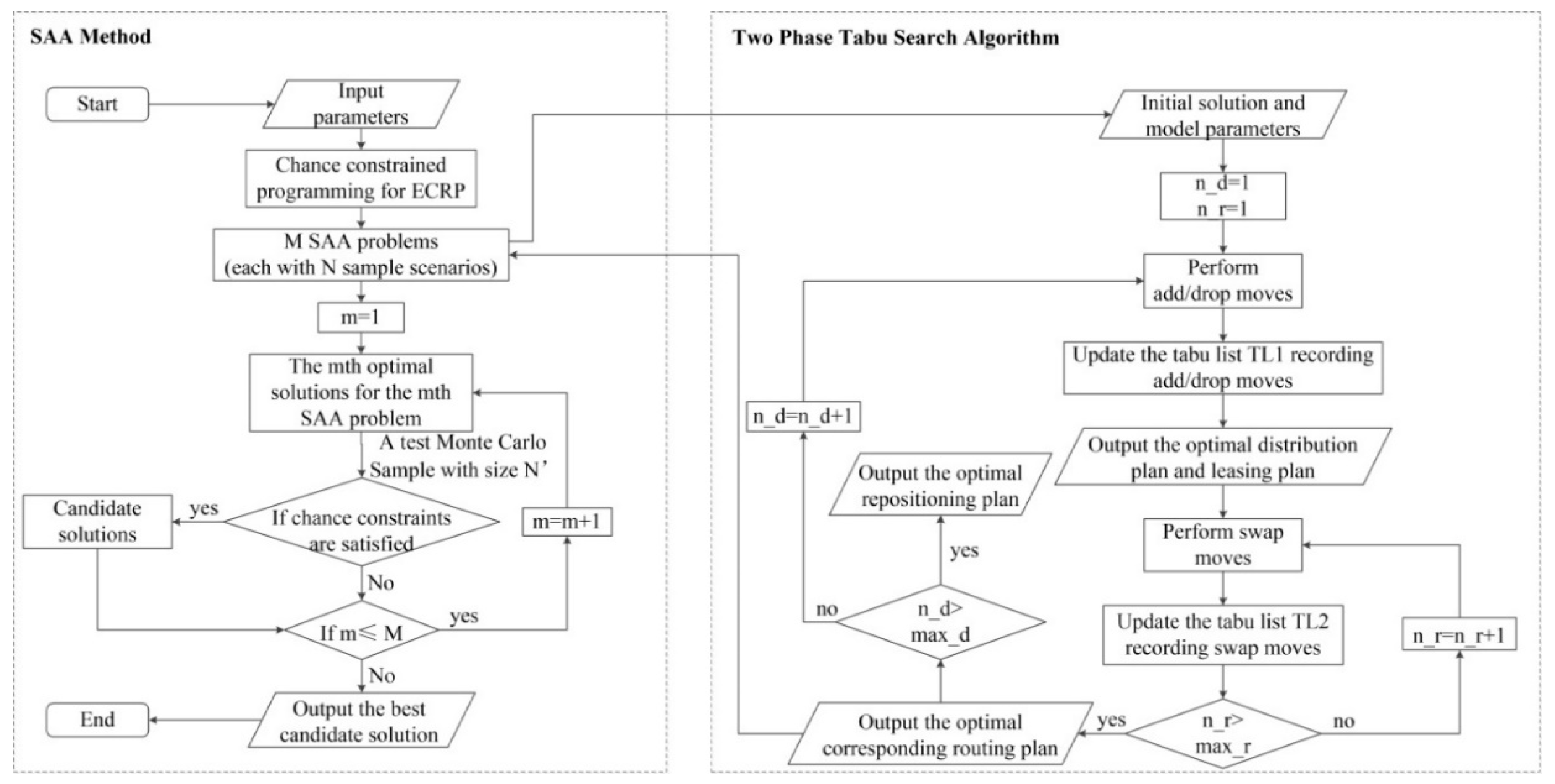
As a mature approach, tabu search algorithm has been extensively applied to transportation operation research, e.g., stop-skipping scheduling problem [47] and vehicle routing problem [48]. Therefore, a two-phase tabu search algorithm is designed to solve the deterministic SAA problem for stochastic ECRP with CO2 emissions, which is composed of a distribution phase and routing phase. The procedure of two-phase tabu search algorithm, incorporating SAA method, is illustrated as a flowchart in Figure 1.
3.2.1. Distribution Phase
In the distribution phase, a tabu search algorithm is developed to determine how many empty containers are required to reposition from surplus nodes to deficit nodes, as well as where and how many empty containers to be leased at deficit nodes, i.e., distribution plan and leasing plan. The main elements are presented, next, in detail.
(i) Neighbourhood structure
In the procedure of tabu search, neighbourhood structure is a key factor for the performance and efficiency of this algorithm, which transforms the current solution into one of its neighbour solutions in the search space [49]. The neighbourhood structure of distribution phase is obtained by considering add or drop moves based on the current solution. Add moves are defined as the moves that increase the amount of repositioned empty containers between one surplus node and one deficit node, while drop moves are described as the moves that decrease the number of repositioned empty containers between two nodes.
For each decision variable of distribution plan , , or , a random number is generated from uniform distribution on the interval (0, 1) to compare with the predetermined selection possibility, which indicates whether an add or drop move is performed for the variable. Then, at each iteration of distribution phase, an add/drop move sample is introduced to represent the move status of all distribution variables. The move status is sorted into three categories: drop move, no move, and add move, corresponding to values −1, 0, and 1, respectively, which the add/drop move sample can take, and the variability range of add or drop moves follows a uniform distribution between 1 TEU and 5 TEUs. Accordingly, all neighbour solutions are obtained, based on the add/drop move sample. For the leasing plan, the corresponding decision variables, and (i.e., the amount of leasing containers at each deficit railway station or port), can be calculated by the difference between the number of repositioned and deficit empty containers. Considering that the leasing cost is time independent, therefore, there is no need to hire surplus empty containers in preparation for the demand of the next time period, which will incur more inventory cost.
(ii) Evaluation of neighbour solutions
To decide which move should be performed, we need to evaluate the objective value of each neighbour solution [50]. In the distribution phase, the handling cost, inventory cost, leasing cost, and CO2 emission-related cost are straightforward and easy to calculate. However, since the routes for transporting empty containers are derived from the routing phase, which is implemented after the distribution phase, the transportation cost is hard to estimate. In order to get a relatively exact evaluation, we assume that each empty container is shipped on the route with the minimal cost. Thus, the evaluation of neighbour solutions is the sum of transportation cost estimate and other component costs.
(iii) Tabu attributes, tabu duration, and aspiration criterion
For add or drop moves in distribution phase, the tabu attribute is the increase or decrease of repositioned empty containers from surplus nodes to deficit nodes, respectively. To avoid the cycling search, a dynamic tabu duration is introduced, which varies with the number of decision variables of the distribution plan. In addition, an aspiration criterion is used to ensure that a tabu add or drop move can be applied when a better solution is found [51].
3.2.2. Routing Phase
The routing phase proposes a tabu search algorithm to specify the routes for transporting the empty containers from surplus nodes to deficit nodes, i.e., a routing plan. The details are stated as follows.
(i) Neighbourhood structure
Considering the characteristics of the binary decision variables of routing phase, swap moves are introduced to obtain the neighbour structure, which transit the current solution to its neighbour solutions in the search space. Swap moves are defined as the moves that specify one candidate route to replace the current route for transporting empty containers. This type of move can ensure that all neighbour solutions satisfy the route selection constraints. Similar to the distribution phase, a swap move sample is employed in this phase to indicate whether a swap move is performed for each decision variable of routing phase, i.e., , , and .
(ii) Evaluation of neighbour solutions
Compared with the distribution phase, the evaluation of neighbour solutions in routing phase is more straightforward. For the given distribution plan and leasing plan, routing phase yields the corresponding optimal routing plan, which only causes the change of transportation cost. Therefore, in order to simplify the calculation and select the best swap move in a highly efficient manner, we use the transportation cost as the evaluation value of each neighbour solution.
(iii) Tabu attributes, tabu duration, and aspiration criterion
For swap moves, the tabu attribute is the changes of routes for transporting empty containers. Since the number of decision variables of distribution phase is relevant with that of routing phase, tabu duration needs to change dynamically to maintain algorithm performance. In the process of searching, if a better solution is encountered, resulting from one tabu swap move, the tabu status of this move will be updated as nontabu, which is defined as an aspiration criterion.
4. Computational Study
In order to demonstrate the proposed chance-constrained nonlinear mixed integer programming model, and evaluate the two-phase tabu search algorithm integrating SAA method, a numerical example is studied in Section 4, considering railway and maritime transportation. In addition, we compare the results of deterministic and stochastic cases, and conduct the sensitivity analyses of model parameters and random variables.
4.1. Deterministic Case
In this section, a sea–rail intermodal network is considered, which consists of seven railway stations and three ports, as shown in Figure 2. The planning horizon T is three time periods, i.e., . At the beginning of the planning horizon, the numbers of empty containers at all nodes are assumed to be zero. Additionally, the unit handling cost, the unit inventory cost, the unit leasing cost, and the unit CO2 emission-related cost are set to be 15 (US$/TEU), 5.6 (US$/TEU), 200 (US$/TEU), and 2 (US$/kg), respectively.
The railway network information is listed in Table 3, including the distance, cost, and CO2 emission when empty containers are transported by train, while the maritime network information is displayed in Table 4, including the port calling sequence of each ship route and the cost and CO2 emission between two ports when empty containers are transported by ship.
It is assumed that three stations (i.e., S1, S2, S3) and three ports (i.e., P1, P2, P3), in this case, are treated as surplus railway station/port or deficit railway station/port, which can generate the demand and supply of empty containers. In other words, the other four stations S4, S5, S6, and S7, are treated as a balanced station/port without repositioning and leasing containers. Table 5 and Table 6 give the demand and supply of empty containers at these six nodes during the planning horizon.
The key parameters of two-phase tabu search algorithm are described as follows. For the distribution phase, the maximum number of iterations max_d and tabu length are set as 100 and 4. For the routing phase, the maximum number of iterations max_r is set as 50, while the tabu length is dependent on the number of routing decision variables at each time period. The solution methodology, incorporating SAA method and two-phase tabu search algorithm, is coded in MATLAB R2012a. The program is run on a 2.5GHz dual core PC with 4GB RAM.
Given the weights of repositioning cost and CO2 emission-related cost , , we can obtain the repositioning plan with a total cost of $65,991, including the distribution plan, routing plan, and leasing plan at each time period, as shown in Table 7. Table 8 lists the costs of the deterministic case, consisting of transportation cost, handling cost, inventory cost, leasing cost, CO2 emission-related cost, and total cost.
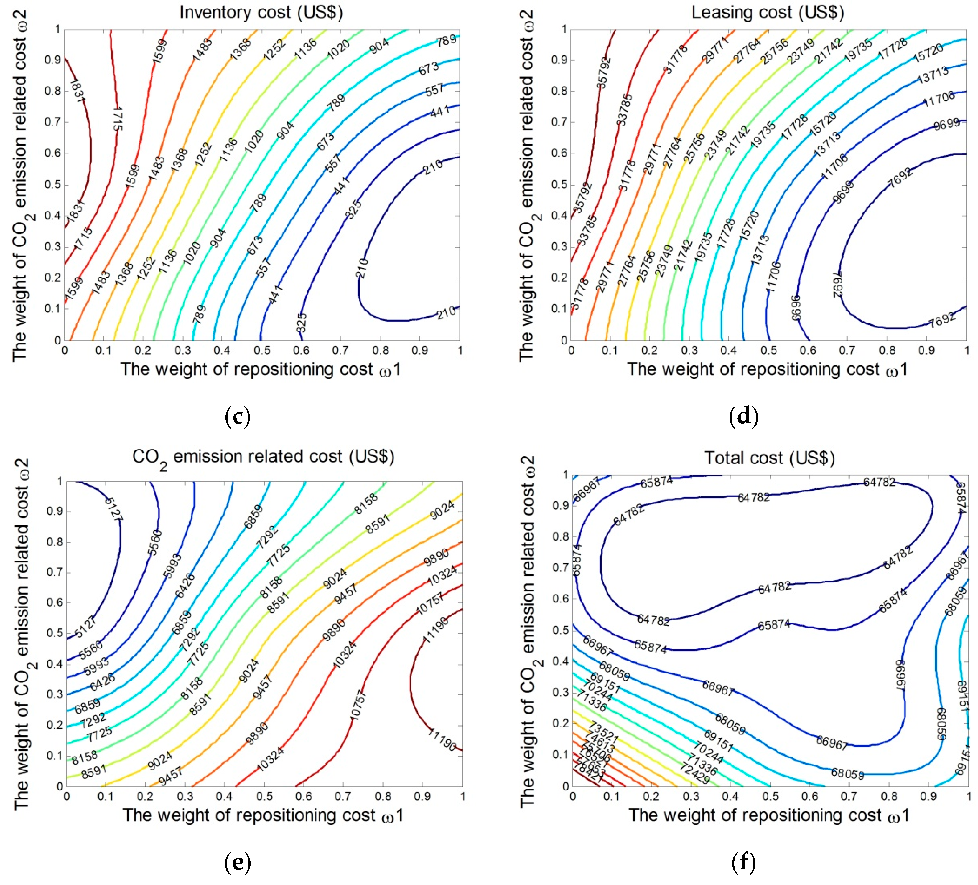
To assess the influence of the weights of repositioning cost and CO2 emission-related cost, we test the deterministic case under different weight combinations. As shown in Figure 3a,b,e, for a given weight , transportation cost, handling cost and CO2 emission-related cost decline with the increasing value of weight . As CO2 emission is only incurred by repositioning empty containers, less empty containers are transported when CO2 emission-related cost dominates the total weighted cost. In other words, when the value of weight goes up, more empty containers are leased to satisfy the demand because it makes no contribution to CO2 emission. As a consequence, the three component costs drop to a low level with the decreasing number of repositioned empty containers, and vice versa.
On the contrary, inventory cost and leasing cost present an increasing tendency, as illustrated in Figure 3c,d. As discussed above, less empty containers are repositioned resulting from the growth of weight . Consequently, it leads to more empty containers accumulating at surplus railway stations or ports, which incur high inventory cost. On the other hand, more leased empty containers undoubtedly result in the rise of leasing cost. As depicted in Figure 3f, compared with other component costs, total cost ascends significantly with the weights and both declining from 0.6 to 0. Nevertheless, it grows slowly when the two weights are larger than 0.6. We conjecture that this can be explained by the interaction of multiple component costs and relevant model parameters. Hence, it is can be concluded that total cost and other component costs are strongly dependent on the weight combinations.
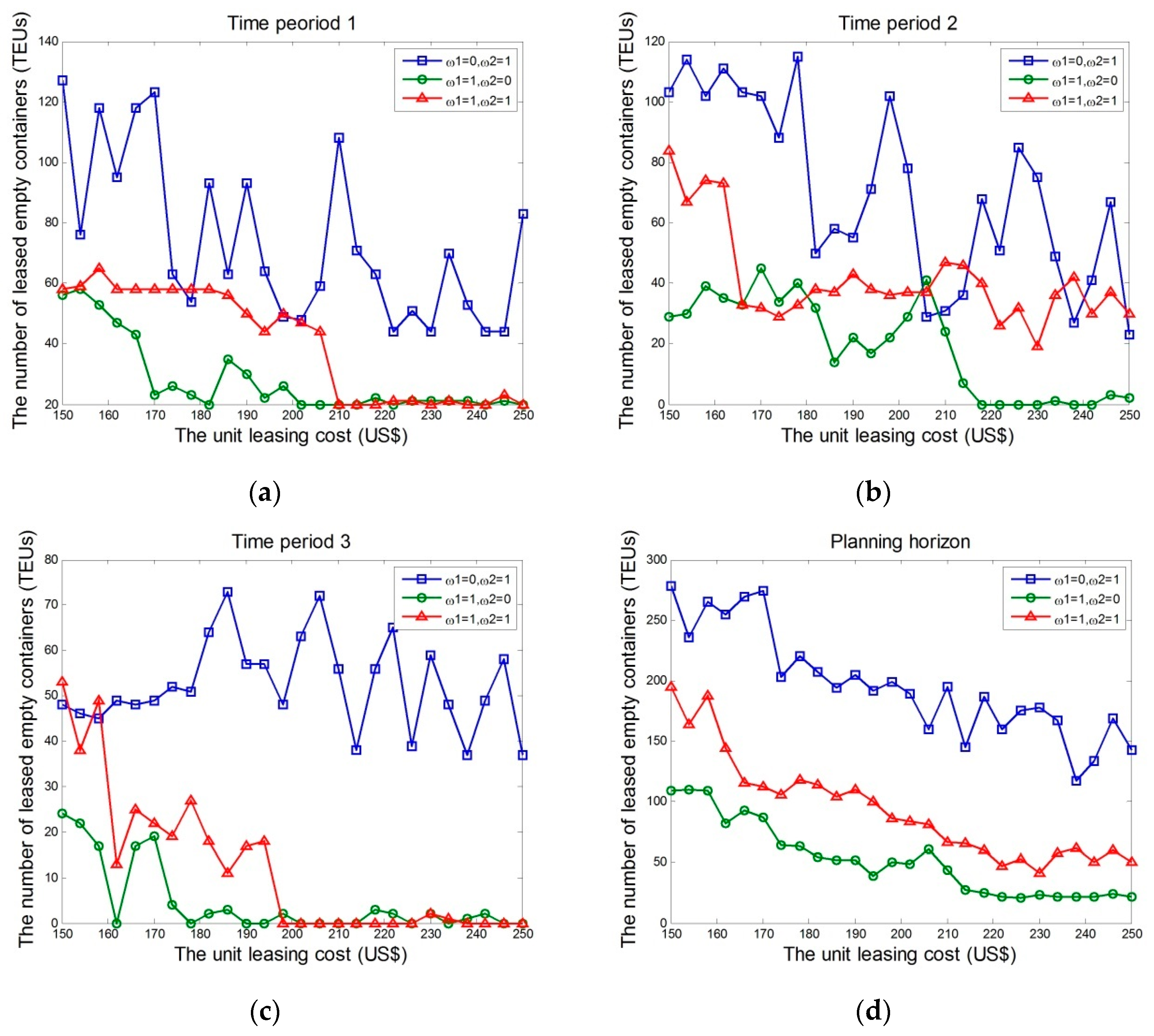
Next, we examine the effect of unit leasing cost on the number of leased empty containers under three different weight combinations for each time period and the whole planning horizon. As expected, the amounts of leased empty containers for the three weight settings all descend with the growth of unit leasing cost in Figure 4. However, for the weight setting , , the number of leased empty containers is less sensitive to the unit leasing cost, and fluctuates fiercely because the change of unit leasing cost cannot affect the total weighted cost when . Furthermore, we note that the number of leased empty containers for the weight setting , is generally more than the other two weight settings. Since the value of for the other two weight settings is 1, that means the leasing cost accounts for a larger percentage of total weighted cost, and freight companies are preferable to repositioned empty containers rather than leased empty containers to reduce high leasing cost.
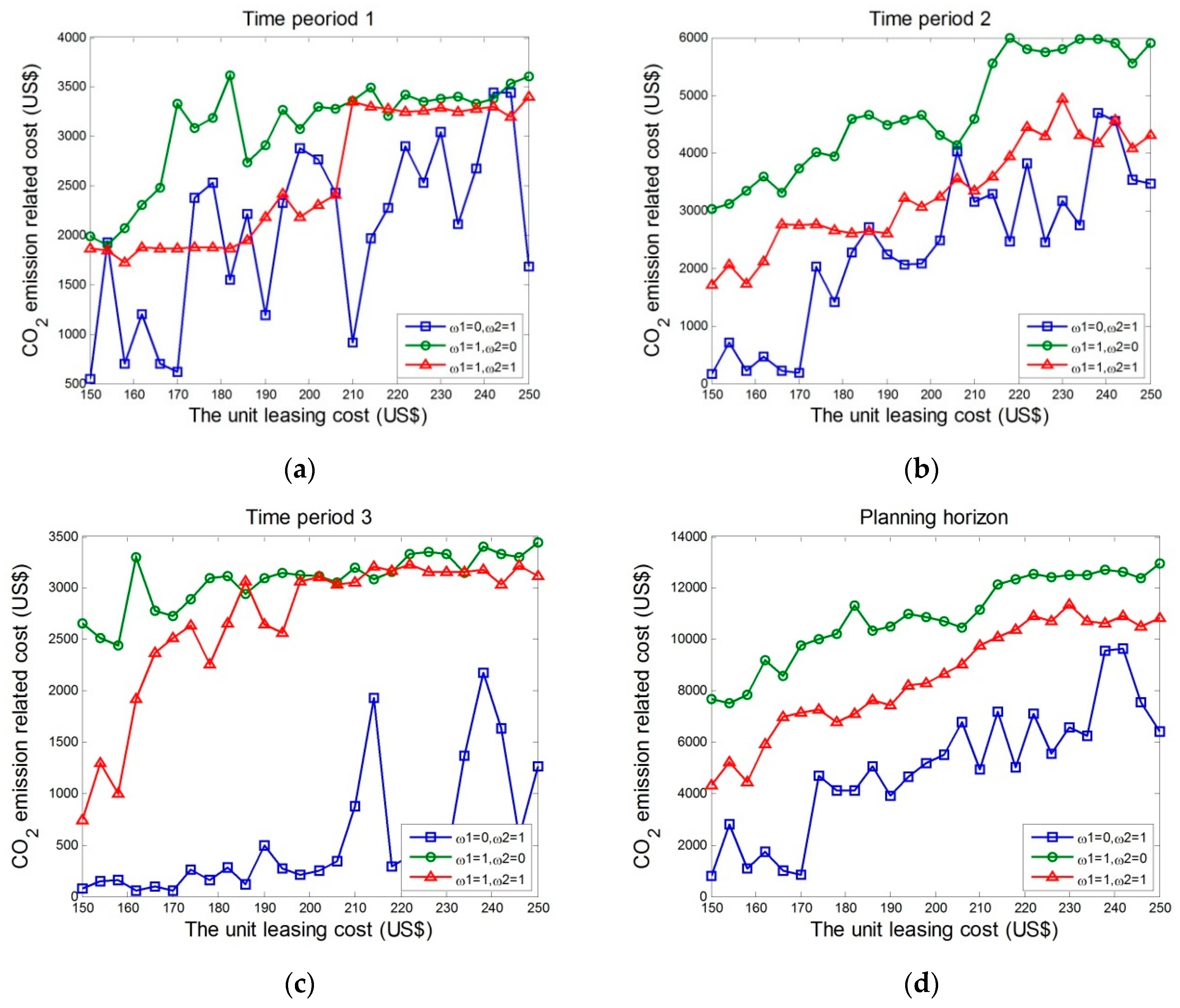
Figure 5 illustrates the influence of unit leasing cost on CO2 emission-related cost under three different weight combinations. As indicated in Figure 5, CO2 emission-related cost grows with the increase of unit leasing cost. This can be explained by less leased empty containers, which forces more empty containers to be repositioned as a complementary way to satisfy the demand. At the same time, more CO2 is emitted during the process of repositioning, resulting in more CO2 emission-related cost.
4.2. Stochastic Case
As mentioned in Section 2.1, the uncertain demand of empty containers and both follow uniform distributions, i.e., , with the demand of deterministic case at railway station i, and , with the demand of deterministic case at port p, where coefficient is defined as the variability of uncertain demand. Similarly, the uncertain supply of empty containers and also follow uniform distributions, i.e., and , where and , the supplies of deterministic case at railway station i and port p, respectively, as well as , the variability of uncertain supply. Here, and both take value 6. For SAA method parameters, we set sample sizes N, , and replication number M, to be 500, 10,000, and 10, respectively. Confidence levels and are both assumed to be 0.5. In addition, other input parameters are the same with those of deterministic case. Table 9 reports the distribution plan, routing plan, and leasing plan of stochastic case at each time period, while Table 10 shows the associated costs.
As compared with the results of deterministic case, stochastic demand and supply result in a different repositioning plan. With respect to the distribution plan, repositioned empty containers rise dramatically from 418 TEUs of deterministic case to 516 TEUs of stochastic case. Similarly, for the leasing plan, leased empty containers grow relatively steadily, from 88 TEUs to 106 TEUs. By contrast, there is no change in the routing plan. Due to the rise of repositioned and leased empty containers, the total cost and other component costs go up considerably in comparison to those of the deterministic case.
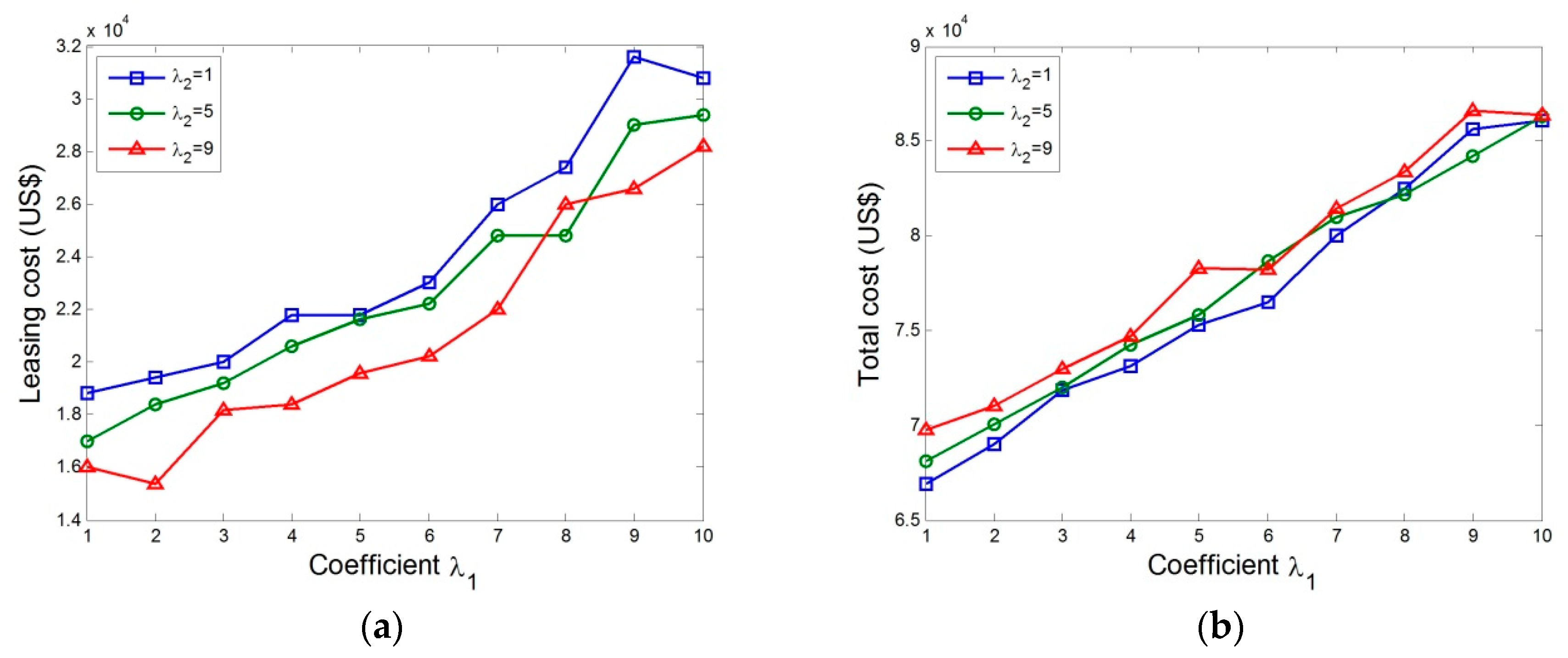
To further investigate the effect of stochasticity, we test the stochastic case with different and , i.e., different variabilities of stochastic demand and supply. As shown in Figure 6, the leasing cost and total cost ascend with coefficient . In Figure 6a, we can also observe that the leasing cost with is always more than those with and , when varies from 1 to 10. This implies that lower supply variability provides less available empty containers than the other two situations, so more leased containers are required to satisfy the demand, which incurs more leasing cost.
Likewise, the effect of coefficient is also analysed. It can be seen from Figure 7 that the inventory cost rises noticeably, while the total cost fluctuates within a certain range and goes up very slightly. In addition, we notice that the total cost with is more than other two situations in Figure 7b, which indicates that more operation cost is requested to cope with higher variability in empty container demand.
5. Conclusions
This paper has presented an empty container repositioning problem (ECRP) allowing for CO2 emissions, and stochastic demand and supply. To formulate this problem, a chance-constrained mixed integer programming model is proposed to minimise the expected value of total weighted cost in a sea–rail intermodal network. In order to solve it, sample average approximation (SAA) method is used to convert it into its deterministic equivalents. Two-phase tabu search algorithm is then developed to obtain the optimal solution of the converted SAA problem. Specifically, the first phase yields the distribution plan and leasing plan, whilst the second phase produces the routing plan. Finally, a computational study has been carried out to validate the proposed model and developed solution methodology. The results indicate that the repositioning plan and total cost are affected not only by stochastic factors, but also by weight combinations. To explore the effect of them, a series of sensitivity analyses is conducted. We conclude that stochastic demand and supply can both increase the transportation cost, handling cost, inventory cost, leasing cost, CO2 emission-related cost, and total cost compared with the deterministic case. At the same time, the amounts of repositioned and leased empty containers also present an increasing tendency. Moreover, the impact of variabilities of stochastic factors on costs is examined. Higher variability of stochastic demand results in more leasing cost and total cost, while higher variability of stochastic supply leads to the increased inventory cost and fluctuating total cost. With respect to the weights of repositioning cost and CO2 emission-related cost, it is found that both of them have a positive or negative relationship with the costs. Transportation cost, handling cost, and CO2 emission-related cost decline with the increasing value of weight and the decrease of weight . By contrast, inventory cost and leasing cost present an opposite trend. Additionally, the results also show that the rise of unit leasing cost can lead to the decrease of the number of leased empty containers, and the increase of CO2 emission-related cost. These findings in this paper can provide implications for decision-makers when an operation plan for repositioning and leasing empty containers needs to be determined in a stochastic environment. Furthermore, the decision-maker can obtain the different repositioning plans under different weight combinations, according to their preferences.
There are two directions which are worth investigating for future research. The first direction is to integrate the routing problem of loaded containers in the decision process of ECRP. The second direction is to consider uncertain factors from the perspective of fuzzy theory.
Author Contributions
Conceptualization, Y.Z.; Methodology, Y.Z. and Q.X.; Validation, Y.Z. and Q.X.; Formal Analysis, Y.Z. and Q.X.; Investigation, Y.Z.; Writing—Original Draft Preparation, Y.Z.; Writing—Review & Editing, Y.Z. and X.Z.; Supervision, X.Z.
Funding
This research received no external funding.
Acknowledgments
We would like to thank Chao Lu (Beijing Jiaotong University) for his technical support.
Conflicts of Interest
The authors declare no conflict of interest.
References
- Zhao, Y.; Liu, R.; Zhang, X.; Whiteing, A. A chance-constrained stochastic approach to intermodal container routing problems. PLoS ONE 2018, 13, e0192275. [Google Scholar] [CrossRef] [PubMed]
- Long, Y.; Lee, L.H.; Chew, E.P. The sample average approximation method for empty container repositioning with uncertainties. Eur. J. Oper. Res. 2012, 222, 65–75. [Google Scholar] [CrossRef]
- Review of Maritime Transportation 2017. UNCTAD 2017. Available online: https://unctad.org/en/PublicationsLibrary/rmt2017_en.pdf (accessed on 15 October 2018).
- Demir, E.; Burgholzer, W.; Hrušovský, M.; Arıkan, E.; Jammernegg, W.; van Woensel, T. A green intermodal service network design problem with travel time uncertainty. Transp. Res. Part B Methodol. 2016, 93, 789–807. [Google Scholar] [CrossRef]
- Wang, Y.; Yan, X.; Zhou, Y.; Xue, Q.; Sun, L. Individuals’ acceptance to free-floating electric carsharing mode: A web-based survey in China. Int. J. Environ. Res. Public Health 2017, 14, 476. [Google Scholar] [CrossRef] [PubMed]
- Third IMO GHG Study 2014: Executive Summary and Final Report. International Maritime Organization 2014. Available online: http://www.imo.org/en/OurWork/Environment/PollutionPrevention/AirPollution/Documents/Third%20Greenhouse%20Gas%20Study/GHG3%20Executive%20Summary%20and%20Report.pdf (accessed on 15 October 2018).
- Huang, Y.F.; Hu, J.K.; Yang, B. Liner services network design and fleet deployment with empty container repositioning. Comput. Ind. Eng. 2015, 89, 116–124. [Google Scholar] [CrossRef]
- Jula, H.; Chassiakos, A.; Ioannou, P. Port dynamic empty container reuse. Transp. Res. Part E Logist. Transp. Rev. 2006, 42, 43–60. [Google Scholar] [CrossRef]
- Feng, C.M.; Chang, C.H. Empty container reposition planning for intra-Asia liner shipping. Marit. Policy Manag. 2008, 35, 469–489. [Google Scholar] [CrossRef]
- Braekers, K.; Janssens, G.K.; Caris, A. Challenges in managing empty container movements at multiple planning levels. Transp. Rev. 2011, 31, 681–708. [Google Scholar] [CrossRef]
- Song, D.P.; Dong, J.X. Empty container repositioning. In Handbook of Ocean Container Transport Logistics; Lee, C.Y., Meng, Q., Eds.; Springer: Cham, Switzerland, 2015; pp. 163–208. ISBN 978-3-319-11890-1. [Google Scholar]
- Florez, H. Empty-container Repositioning and Leasing: An Optimization Model. Ph.D. Thesis, Polytechnic-Institute of New York, Brooklyn, NY, USA, 1986. [Google Scholar]
- Crainic, T.G.; Delorme, L. Dual-ascent procedures for multicommodity location-allocation problems with balancing requirements. Transp. Sci. 1993, 27, 90–101. [Google Scholar] [CrossRef]
- Shintani, K.; Imai, A.; Nishimura, E.; Papadimitriou, S. The container shipping network design problem with empty container repositioning. Transp. Res. Part E Logist. Transp. Rev. 2007, 43, 39–59. [Google Scholar] [CrossRef]
- Song, D.P.; Carter, J. Empty container repositioning in liner shipping. Marit. Policy Manag. 2009, 36, 291–307. [Google Scholar] [CrossRef]
- Moon, I.K.; Do Ngoc, A.D.; Hur, Y.S. Positioning empty containers among multiple ports with leasing and purchasing considerations. OR Spectr. 2010, 32, 765–786. [Google Scholar] [CrossRef]
- Brouer, B.D.; Pisinger, D.; Spoorendonk, S. Liner shipping cargo allocation with repositioning of empty containers. INFOR: Inf. Syst. Oper. Res. 2011, 49, 109–124. [Google Scholar] [CrossRef]
- Meng, Q.; Wang, S. Liner shipping service network design with empty container repositioning. Transp. Res. Part E Logist. Transp. Rev. 2011, 47, 695–708. [Google Scholar] [CrossRef]
- Song, D.P.; Dong, J.X. Cargo routing and empty container repositioning in multiple shipping service routes. Transp. Res. Part B Methodol. 2012, 46, 1556–1575. [Google Scholar] [CrossRef]
- Song, D.P.; Dong, J.X. Long-haul liner service route design with ship deployment and empty container repositioning. Transp. Res. Part B Methodol. 2013, 55, 188–211. [Google Scholar] [CrossRef]
- An, F.; Hu, H.; Xie, C. Service network design in inland waterway liner transportation with empty container repositioning. Eur. Transp. Res. Rev. 2015, 7, 9. [Google Scholar] [CrossRef]
- Cheung, R.K.; Chen, C.Y. A two-stage stochastic network model and solution methods for the dynamic empty container allocation problem. Transp. Sci. 1998, 32, 142–162. [Google Scholar] [CrossRef]
- Crainic, T.G.; Gendreau, M.; Dejax, P. Dynamic and stochastic models for the allocation of empty containers. Oper. Res. 1993, 41, 102–126. [Google Scholar] [CrossRef]
- Li, J.A.; Liu, K.; Leung, S.C.; Lai, K.K. Empty container management in a port with long-run average criterion. Math. Comput. Model. 2004, 40, 85–100. [Google Scholar] [CrossRef]
- Li, J.A.; Leung, S.C.; Wu, Y.; Liu, K. Allocation of empty containers between multi-ports. Eur. J. Oper. Res. 2007, 182, 400–412. [Google Scholar] [CrossRef]
- Song, D.P. Characterizing optimal empty container reposition policy in periodic-review shuttle service systems. J. Oper. Res. Soc. 2007, 58, 122–133. [Google Scholar] [CrossRef]
- Lam, S.W.; Lee, L.H.; Tang, L.C. An approximate dynamic programming approach for the empty container allocation problem. Transp. Res. Part C Emerg. Technol. 2007, 15, 265–277. [Google Scholar] [CrossRef]
- Song, D.P.; Dong, J.X. Empty container management in cyclic shipping routes. Marit. Econ. Logist. 2008, 10, 335–361. [Google Scholar] [CrossRef]
- Di Francesco, M.; Crainic, T.G.; Zuddas, P. The effect of multi-scenario policies on empty container repositioning. Transp. Res. Part E Logist. Transp. Rev. 2009, 45, 758–770. [Google Scholar] [CrossRef]
- Song, D.P.; Zhang, Q. A fluid flow model for empty container repositioning policy with a single port and stochastic demand. SIAM J. Control Optim. 2010, 48, 3623–3642. [Google Scholar] [CrossRef]
- Song, D.P.; Dong, J.X. Flow balancing-based empty container repositioning in typical shipping service routes. Marit. Econ. Logist. 2011, 13, 61–77. [Google Scholar] [CrossRef]
- Lee, L.H.; Chew, E.P.; Luo, Y. Empty container management in multi-port system with inventory-based control. Int. J. Adv. Syst. Meas. 2012, 5, 164–177. [Google Scholar]
- Dong, J.X.; Xu, J.; Song, D.P. Assessment of empty container repositioning policies in maritime transport. Int. J. Logist. Manag. 2013, 24, 49–72. [Google Scholar] [CrossRef]
- Sainz Bernat, N.; Schulte, F.; Voß, S.; Böse, J. Empty container management at ports considering pollution, repair options, and street-turns. Math. Probl. Eng. 2016. [Google Scholar] [CrossRef]
- Choong, S.T.; Cole, M.H.; Kutanoglu, E. Empty container management for intermodal transportation networks. Transp. Res. Part E Logist. Transp. Rev. 2002, 38, 423–438. [Google Scholar] [CrossRef] [Green Version]
- Meng, Q.; Wang, S.; Liu, Z. Network design for shipping service of large-scale intermodal liners. Transp. Res. Rec. 2012, 2269, 42–50. [Google Scholar] [CrossRef]
- Braekers, K.; Caris, A.; Janssens, G.K. Optimal shipping routes and vessel size for intermodal barge transport with empty container repositioning. Comput. Ind. 2013, 64, 155–164. [Google Scholar] [CrossRef] [Green Version]
- Kolar, P.; Schramm, H.J.; Prockl, G. Intermodal transport and repositioning of empty containers in Central and Eastern Europe hinterland. J. Transp. Geogr. 2018, 69, 73–82. [Google Scholar] [CrossRef]
- Dong, J.X.; Song, D.P. Quantifying the impact of inland transport times on container fleet sizing in liner shipping services with uncertainties. OR Spectr. 2012, 34, 155–180. [Google Scholar] [CrossRef]
- Xie, Y.; Liang, X.; Ma, L.; Yan, H. Empty container management and coordination in intermodal transport. Eur. J. Oper. Res. 2017, 257, 223–232. [Google Scholar] [CrossRef]
- Song, D.P.; Xu, J. An operational activity-based method to estimate CO2 emissions from container shipping considering empty container repositioning. Transp. Res. Part D Transp. Environ. 2012, 17, 91–96. [Google Scholar] [CrossRef]
- Charnes, A.; Cooper, W.W. Chance-constrained programming. Manag. Sci. 1959, 6, 73–79. [Google Scholar] [CrossRef]
- Kleywegt, A.J.; Shapiro, A.; Homem-de-Mello, T. The sample average approximation method for stochastic discrete optimization. SIAM J. Optim. 2002, 12, 479–502. [Google Scholar] [CrossRef]
- Verweij, B.; Ahmed, S.; Kleywegt, A.J.; Nemhauser, G.; Shapiro, A. The sample average approximation method applied to stochastic routing problems: A computational study. Comput. Optim. Appl. 2003, 24, 289–333. [Google Scholar] [CrossRef]
- Pagnoncelli, B.K.; Ahmed, S.; Shapiro, A. Sample average approximation method for chance constrained programming: Theory and applications. J. Optim. Theory Appl. 2009, 142, 399–416. [Google Scholar] [CrossRef]
- Luedtke, J.; Ahmed, S. A sample approximation approach for optimization with probabilistic constraints. SIAM J. Optim. 2008, 19, 674–699. [Google Scholar] [CrossRef]
- Cao, Z.; Yuan, Z.; Zhang, S. Performance analysis of stop-skipping scheduling plans in rail transit under time-dependent demand. Int. J. Environ. Res. Public Health 2016, 13, 707. [Google Scholar] [CrossRef] [PubMed]
- Shen, L.; Tao, F.; Wang, S. Multi-Depot Open Vehicle Routing Problem with Time Windows Based on Carbon Trading. Int. J. Environ. Res. Public Health 2018, 15, 2025. [Google Scholar] [CrossRef] [PubMed]
- Crainic, T.G.; Gendreau, M.; Soriano, P.; Toulouse, M. A tabu search procedure for multicommodity location/allocation with balancing requirements. Ann. Oper. Res. 1993, 41, 359–383. [Google Scholar] [CrossRef]
- Pedersen, M.B.; Crainic, T.G.; Madsen, O.B. Models and tabu search metaheuristics for service network design with asset-balance requirements. Transp. Sci. 2009, 43, 158–177. [Google Scholar] [CrossRef]
- Sun, M.; Aronson, J.E.; McKeown, P.G.; Drinka, D. A tabu search heuristic procedure for the fixed charge transportation problem. Eur. J. Oper. Res. 1998, 106, 441–456. [Google Scholar] [CrossRef]
Figure 1.
The flowchart of heuristic solution methodology.

Figure 2.
A sea–rail intermodal network.
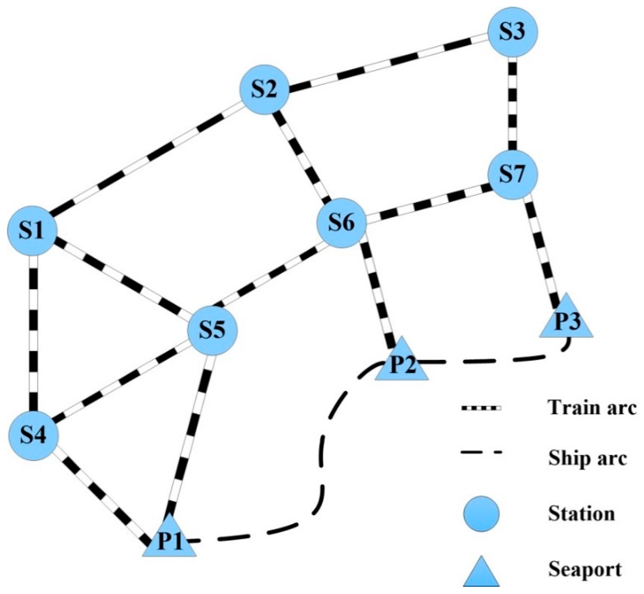
Figure 3.
The costs under different weight combinations. (a) Transportation cost under different weight combinations; (b) Handling cost under different weight combinations; (c) Inventory cost under different weight combinations; (d) Leasing cost under different weight combinations; (e) CO2 emission-related cost under different weight combinations; (f) Total cost under different weight combinations.


Figure 4.
The impact of unit leasing cost on the number of leased empty containers under different weight combinations. (a) The number of leased empty containers at time period 1; (b) The number of leased empty containers at time period 2; (c) The number of leased empty containers at time period 3; (d) The number of leased empty containers during the planning horizon.

Figure 5.
The influence of unit leasing cost on CO2 emission-related cost under different weight combinations. (a) CO2 emission-related cost at time period 1; (b) CO2 emission-related cost at time period 2; (c) CO2 emission-related cost at time period 3; (d) CO2 emission-related cost during the planning horizon.

Figure 6.
The comparisons of leasing cost and total cost with different coefficient λ1. (a) Leasing cost with different coefficient λ1; (b) Total cost with different coefficient λ1.
Figure 6.
The comparisons of leasing cost and total cost with different coefficient λ1. (a) Leasing cost with different coefficient λ1; (b) Total cost with different coefficient λ1.

Figure 7.
The comparisons of inventory cost and total cost with different coefficient λ2. (a) Inventory cost with different coefficient λ2; (b) Total cost with different coefficient λ2.
Figure 7.
The comparisons of inventory cost and total cost with different coefficient λ2. (a) Inventory cost with different coefficient λ2; (b) Total cost with different coefficient λ2.


Table 1.
The literature review of empty container repositioning.
| Transportation Mode | Stochastic Demand and/or Supply | CO2 Emissions | Key References |
|---|---|---|---|
| Unimodal | No | No | Huang et al. [7]; Jula et al. [8]; Feng and Chang [9]; Florez [12]; Crainic and Delorme [13]; Shintani et al. [14]; Song and Carter [15]; Moon et al. [16]; Brouer et al. [17]; Meng and Wang [18]; Song and Dong [19,20]; An et al. [21] |
| Unimodal | Yes | No | Long et al. [2]; Cheung and Chen [22]; Crainic et al. [23]; Li et al. [24]; Li et al. [25]; Song [26]; Lam et al. [27]; Song and Dong [28]; Francesco et al. [29]; Song and Zhang [30]; Song and Dong [31]; Lee et al. [32]; Dong et al. [33] |
| Unimodal | Yes | Yes | Bernat et al. [34] |
| Intermodal | No | No | Choong et al. [35]; Meng et al. [36]; Braekers et al. [37]; Kolar et al. [38] |
| Intermodal | Yes | No | Dong and Song [39]; Xie et al. [40] |
| Intermodal | Yes | Yes | This paper |
Table 2.
Notations.
| Term | Definition |
|---|---|
| Index and set | |
| the set of nodes, | |
| the set of railway stations | |
| the set of ports | |
| the set of railway stations with surplus empty containers, | |
| the set of railway stations with deficit empty containers, | |
| the set of ports with surplus empty containers, | |
| the set of ports with deficit empty containers, | |
| the set of arcs, | |
| the set of railway arcs, including the arcs between two railway stations and the arcs between one railway station and one port | |
| the set of ship arcs, i.e., the arcs between two ports | |
| the sets of candidate railway routes between two railway stations and from one railway station to one port, distinguished by the origin stations, destination railway stations/ports, and intermediate railway stations. | |
| the set of candidate ship routes distinguished by their port calling sequences | |
| the planning horizon | |
| two railway stations, | |
| two ports, | |
| a transportation arc, | |
| a candidate railway route, | |
| a candidate ship route, | |
| a time period, | |
| Input parameters | |
| the distance of arc a (km) | |
| the unit transportation cost of one empty container on railway arc a, (US$/TEU) | |
| the unit transportation cost of one empty container on ship arc a of ship route r (US$/TEU) | |
| the unit loading cost of one empty container at railway station i (US$/TEU) | |
| the unit unloading cost of one empty container at railway station j (US$/TEU) | |
| the unit loading cost of one empty container at port p (US$/TEU) | |
| the unit unloading cost of one empty container at port q (US$/TEU) | |
| the unit inventory cost of storing one empty container per time period at railway station i (US$/TEU) | |
| the unit inventory cost of storing one empty container per time period at port p (US$/TEU) | |
| the unit leasing cost of one empty container at railway station i (US$/TEU) | |
| the unit leasing cost of one empty container at port p (US$/TEU) | |
| the unit CO2 emission-related cost (US$/kg) | |
| the CO2 emissions of arc a (kg/TEU) | |
| the transportation capacity of railway arc a (TEUs) | |
| the transportation capacity of ship route r when one ship is deployed (TEUs) | |
| the handling capacity of railway station i, including loading and unloading operations (TEUs) | |
| the handling capacity of port p, including loading and unloading operations (TEUs) | |
| the inventory capacity of railway station i (TEUs) | |
| the inventory capacity of port p (TEUs) | |
| the number of empty containers stored at railway station i at the end of time t (TEUs) | |
| the number of empty containers stored at port p at the end of time t (TEUs) | |
| a binary variable, equal to 1 if the arc a is on the railway route k; 0 otherwise | |
| a binary variable, equal to 1 if the arc a is on the ship route r; 0 otherwise | |
| Random variables | |
| the uncertain demand of empty containers at railway station i at time t (TEUs) | |
| the uncertain supply of empty containers at railway station i at time t (TEUs) | |
| the uncertain demand of empty containers at port p at time t (TEUs) | |
| the uncertain supply of empty containers at port p at time t (TEUs) | |
| Decision variables | |
| the number of repositioned empty containers by train from i to j at time t | |
| the number of repositioned empty containers by ship from p to q at time t | |
| the number of repositioned empty containers by train from i to q at time t | |
| a binary variable, equal to 1 if railway route k is selected to transport empty containers from i to j at time t; 0 otherwise | |
| a binary variable, equal to 1 if ship route r is selected to transport empty containers from p to q at time t; 0 otherwise | |
| a binary variable, equal to 1 if railway route k is selected to transport empty containers from i to q at time t; 0 otherwise | |
| the number of leased empty containers at railway station i at time t | |
| the number of leased empty containers at port p at time t | |
| the vector of all decision variables at time t, i.e., |
Table 3.
The railway network information.
| Arc | Distance (km) | Cost (US$/TEU) | CO2 (kg/TEU) |
|---|---|---|---|
| (S1, S2) | 195 | 59.25 | 9.86 |
| (S1, S4) | 158 | 53.7 | 7.99 |
| (S1, S5) | 158 | 53.7 | 7.99 |
| (S2, S3) | 190 | 58.5 | 9.61 |
| (S2, S6) | 98 | 44.7 | 5 |
| (S3, S7) | 88 | 43.2 | 4.45 |
| (S4, S5) | 145 | 51.75 | 7.34 |
| (S4, P1) | 135 | 50.25 | 6.83 |
| (S5, S6) | 100 | 45 | 5.06 |
| (S5, P1) | 165 | 54.75 | 8.35 |
| (S6, S7) | 100 | 45 | 5.06 |
| (S6, P2) | 100 | 45 | 5.06 |
| (S7, P3) | 100 | 45 | 5.06 |
Table 4.
The maritime network information.
| Ship Route | Port Calling Sequence | Arc | Cost (US$/TEU) | CO2 (kg/TEU) |
|---|---|---|---|---|
| 1 | P1→P2→P1 | (P1, P2) | 18 | 9.75 |
| 2 | P2→P3→P2 | (P2, P3) | 15 | 3.68 |
| 3 | P1→P3→P1 | (P1, P3) | 30 | 13.43 |
| 4 | P1→P2→P3→P2→P1 | (P1, P2) | 17 | 9.75 |
| (P2, P3) | 16 | 3.68 |
Table 5.
The demand of empty containers at each time period.
| Demand of Empty Containers (TEUs) | S1 | S2 | S3 | P1 | P2 | P3 |
|---|---|---|---|---|---|---|
| t = 1 | 424 | 428 | 392 | 490 | 446 | 632 |
| t = 2 | 396 | 324 | 414 | 530 | 548 | 454 |
| t = 3 | 378 | 292 | 406 | 582 | 532 | 594 |
Table 6.
The supply of empty containers at each time period.
| Supply of Empty Containers (TEUs) | S1 | S2 | S3 | P1 | P2 | P3 |
|---|---|---|---|---|---|---|
| t = 1 | 366 | 368 | 436 | 464 | 552 | 606 |
| t = 2 | 436 | 276 | 316 | 622 | 466 | 550 |
| t = 3 | 336 | 328 | 356 | 628 | 586 | 550 |
Table 7.
The repositioning plan of the deterministic case.
| Time Period t | Distribution Plan | Routing Plan | Leasing Plan |
|---|---|---|---|
| 1 | S3→S1: 10 TEUs | S3→S2→S1 | S1: 48 TEUs |
| S3→S2: 34 TEUs | S3→S2 | ||
| P2→S2: 26 TEUs | P2→S6→S2 | ||
| P2→P1: 26 TEUs | Ship route 4 | ||
| P2→P3: 26 TEUs | Ship route 2 | ||
| 2 | S1→S2: 20 TEUs | S1→S2 | S2: 18 TEUs S3: 22 TEUs |
| S1→S3: 20 TEUs | S1→S2→S3 | ||
| P1→P2: 24 TEUs | Ship route 4 | ||
| P3→S2: 10 TEUs | P3→S7→S6→S2 | ||
| P3→S3: 56 TEUs | P3→S7→S3 | ||
| P3→P2: 30 TEUs | Ship route 2 | ||
| 3 | S2→S3: 36 TEUs | S2→S3 | - |
| P1→S1: 42 TEUs | P1→S4→S1 | ||
| P1→P3: 22 TEUs | Ship route 3 | ||
| P2→S3: 14 TEUs | P2→S6→S7→S3 | ||
| P2→P3: 22 TEUs | Ship route 2 |
Table 8.
The costs of the deterministic case.
| Time Period t | Transportation Cost (US$) | Handling Cost (US$) | Inventory Cost (US$) | Leasing Cost (US$) | CO2 Emission-Related Cost (US$) | Total Cost (US$) |
|---|---|---|---|---|---|---|
| 1 | 6330.7 | 3600 | 156.8 | 9600 | 2264.4 | 22,012 |
| 2 | 10,684 | 4800 | 380.8 | 8000 | 3229.5 | 27,095 |
| 3 | 9326.7 | 4080 | 380.8 | 0 | 3097.6 | 16,885 |
| Total | 26,342 | 12,540 | 918.4 | 17,600 | 8591.5 | 65,991 |
Table 9.
The repositioning plan of the stochastic case.
| Time Period t | Distribution Plan | Routing Plan | Leasing Plan |
|---|---|---|---|
| 1 | S3→S1: 16 TEUs | S3→S2→S1 | S1: 48 TEUs S2: 3 TEUs |
| S3→S2: 27 TEUs | S3→S2 | ||
| P2→S2: 36 TEUs | P2→S6→S2 | ||
| P2→P1: 32 TEUs | Ship route 4 | ||
| P2→P3: 32 TEUs | Ship route 2 | ||
| 2 | S1→S2: 24 TEUs | S1→S2 | S2: 22 TEUs S3: 26 TEUs |
| S1→S3: 21 TEUs | S1→S2→S3 | ||
| P1→P2: 56 TEUs | Ship route 4 | ||
| P3→S2: 8 TEUs | P3→S7→S6→S2 | ||
| P3→S3: 62 TEUs | P3→S7→S3 | ||
| P3→P2: 32 TEUs | Ship route 2 | ||
| 3 | S2→S1: 16 TEUs | S2→S1 | S1: 2 TEUs S3: 5 TEUs |
| S2→S3: 30 TEUs | S2→S3 | ||
| P1→S1: 41 TEUs | P1→S4→S1 | ||
| P1→P3: 32 TEUs | Ship route 3 | ||
| P2→S3: 21 TEUs | P2→S6→S7→S3 | ||
| P2→P3: 30 TEUs | Ship route 2 |
Table 10.
The costs of the stochastic case.
| Time Period t | Transportation Cost (US$) | Handling Cost (US$) | Inventory Cost (US$) | Leasing Cost (US$) | CO2 Emission-Related Cost (US$) | Total Cost (US$) |
|---|---|---|---|---|---|---|
| 1 | 7716.7 | 4290 | 177.1 | 10,200 | 2725.8 | 25,110 |
| 2 | 11,873 | 6090 | 459.3 | 9600 | 4039.7 | 32,062 |
| 3 | 11,172 | 5100 | 503.4 | 1400 | 3799.6 | 21,975 |
| Total | 30,762 | 15,480 | 1139.8 | 21200 | 10,565 | 79,147 |
© 2018 by the authors. Licensee MDPI, Basel, Switzerland. This article is an open access article distributed under the terms and conditions of the Creative Commons Attribution (CC BY) license (http://creativecommons.org/licenses/by/4.0/).
Share and Cite
MDPI and ACS Style
Zhao, Y.; Xue, Q.; Zhang, X. Stochastic Empty Container Repositioning Problem with CO2 Emission Considerations for an Intermodal Transportation System. Sustainability 2018, 10, 4211. https://doi.org/10.3390/su10114211
AMA Style
Zhao Y, Xue Q, Zhang X. Stochastic Empty Container Repositioning Problem with CO2 Emission Considerations for an Intermodal Transportation System. Sustainability. 2018; 10(11):4211. https://doi.org/10.3390/su10114211
Chicago/Turabian StyleZhao, Yi, Qingwan Xue, and Xi Zhang. 2018. "Stochastic Empty Container Repositioning Problem with CO2 Emission Considerations for an Intermodal Transportation System" Sustainability 10, no. 11: 4211. https://doi.org/10.3390/su10114211
Note that from the first issue of 2016, this journal uses article numbers instead of page numbers. See further details here.