


Abstract
As space systems evolve towards cis-lunar missions and beyond, the demand for precise yet low-size, -weight, and -power (SWaP) clocks and synchronization methods becomes increasingly critical. We introduce a novel clock synchronization approach based on the Kuramoto oscillator model that facilitates the creation of an ensemble timescale for satellite constellations. Unlike traditional ensembling algorithms, the proposed Kuramoto method leverages nearest-neighbor interactions to achieve collective synchronization. This method simplifies the communication architecture and data-sharing requirements, making it well suited for dynamically connected networks such as proliferated low Earth orbit (pLEO) and lunar or Martian constellations, where intersatellite links may frequently change. Through simulations incorporating realistic noise models for small-scale atomic clocks, we demonstrate that the Kuramoto ensemble can yield an improvement in stability on the order of 1/√N, while mitigating the impact of constellation fragmentation and defragmentation. The results indicate that the Kuramoto oscillator-based algorithm can potentially deliver performance comparable to established techniques like Equal Weights Frequency Averaging (EWFA), yet with enhanced scalability and resource efficiency critical for future spaceborne PNT and communication systems.
1. Introduction
As space-system engineers begin to design Position, Navigation and Timing (PNT) and communication systems for the cis-lunar environment and eventually Mars, the devices employed for precise timekeeping on spacecraft will be severely constrained by size, weight and power (SWaP). Specifically, lunar and Martian orbiting satellites will be considerably smaller than their GNSS terrestrial cousins (i.e., global navigation satellite systems), though their mission requirements (and consequently timekeeping specifications) will be similar [1]. Consequently, the systems engineer will likely need to look to satellite-clock ensembling to meet their missions’ needs, where clocks on different spacecraft average their time readings via satellite crosslinks to create a timescale that is more reliable and stable than what would be created by an individual clock acting alone. In a similar vein, proliferated LEO (pLEO) constellations may also be SWaP constrained but with strict requirements for tight timekeeping that is independent of any GNSS.
All of these constellations will provide ensembling complications that the more traditional ensembling algorithms rarely, if ever, deal with. Specifically, there will be dynamically changing connections between ensemble members due to extra-terrestrial and pLEO satellite orbits and, consequently, the number of satellites contributing to the ensemble timescale will vary as intersatellite links are broken and then reformed. Moreover, with large pLEO constellations, the number of ensemble members could easily grow into the thousands, requiring large computational times (and hence computing power) on each satellite to arrive at a converged timescale solution. Finally, extra-terrestrial and pLEO constellations will likely have high satellite turnovers, meaning that the satellites will stay in orbit for relatively short time periods (e.g., a few years) before being replaced. Consequently, well-characterized clocks will leave and new clocks will enter the ensemble much more often than is “normal” for traditional ensembling algorithms.
Current state-of-the-art clock ensembling algorithms are primarily employed at national laboratories in well-controlled environments and with clocks of roughly similar quality. These algorithms include Kalman filter algorithms [2,3,4], along with specially designed algorithms like NIST’s AT1 and AT2 algorithms [5] and the PTB timescale algorithm [6]. In these algorithms, weights are dynamically applied to the clocks in the ensemble, effectively ranking the quality of an ensemble member based on the agreement between a prediction of its time correction and the actual time correction that is applied by the algorithm. In addition, the Leader–Follower algorithm has been suggested as a possible space system ensemble algorithm [7] where one clock is designated the Leader (for some set time period) and all other clocks “follow the leader.” After a pre-determined time interval, a new Leader is chosen (with the new Leader defined by a low variance of corrections while acting as a Follower). In the Leader–Follower algorithm, advantage is taken of the ergodic theorem: a time average over many different Leaders equals an “instantaneous” ensemble average over many weighted ensemble members.
Regardless of the details, all of these algorithms require the timescale to be constructed by statistically independent clocks. Thus, each satellite in the constellation needs to know the entire history of corrections that all satellites in the constellation apply. Each satellite must then use these correction histories to re-create (in software) what would have been the free-running history of all the ensemble members. This can put a tremendous burden on the amount of data that needs to be transmitted via crosslinks, along with the memory and data processing each satellite must employ to create the ensemble timescale, which can be prohibitive when discussing constellations of hundreds to thousands of satellites. Moreover, this whole issue raises serious questions regarding the loss or corruption of transmitted data on the efficacy of the ensemble algorithm.
To mitigate these space system ensembling problems, we discuss here an alternative: the Kuramoto ensembling algorithm. As will be apparent in what follows, a Kuramoto timescale is easily extendable to large numbers of satellites. In addition, the amount of data needed for the timescale to converge on any one satellite is minimal, since each Kuramoto node (i.e., satellite) only needs information from its nearest neighbors. Our Kuramoto ensembling algorithm is based on the Kuramoto oscillator [8,9,10], which utilizes a synchronization phenomenon whereby non-linear feedback between oscillators causes collective synchronization. The subject of the Kuramoto oscillator has been employed to study a variety of synchronization phenomena such as firefly blinking [11,12], neuron activity [13,14] and coupled metronomes [15,16]. However, to date, no one has considered extending the Kuramoto oscillator concept to ensemble timekeeping.
For space systems, the great advantage of a Kuramoto ensemble algorithm lies in the fact that information about the ensemble members need not be shared globally, nor is there a need to re-create a history of statistically independent (i.e., free running) ensemble members. In other words, a clock only needs information about its nearest neighbors and only at the present epoch. Thus, for a constellation of crosslinked satellites, an ensemble node (i.e., satellite) only needs to know its time offset from its crosslinked neighbors. As each ensemble member steers to the average of itself and its crosslinked neighbors, there is a non-linear coupling among all the ensemble members that results in synchronization.
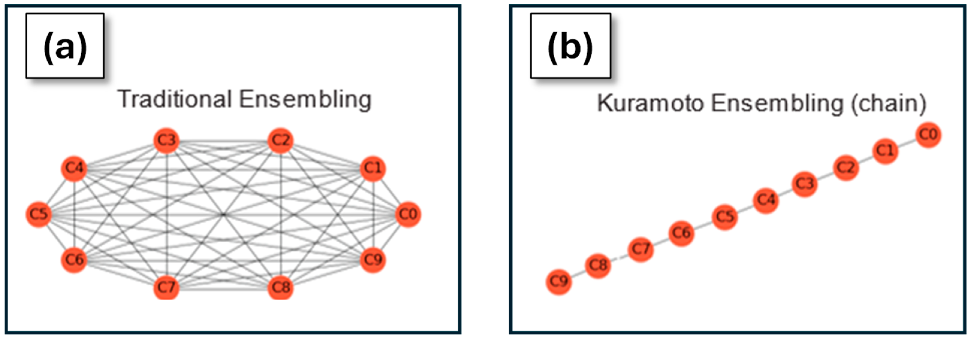
As illustrated in Figure 1, traditional ensemble algorithms can be represented by a diagram where information must flow from one node (i.e., clock) to all other nodes. Alternatively, informational connections for the Kuramoto oscillator system are much simpler and can be illustrated by a simple line or closed-loop node-connection diagram. We note, however, that a Kuramoto ensemble algorithm is not restricted to a linear or closed-loop node-connections. More complicated connection topologies can be employed based on the specifics of the space-system timekeeping architecture.
Figure 1.
These diagrams show information flow for traditional ensembling algorithms (a) and a simple Kuramoto ensembling algorithm (b). The complexity of informational flow for traditional ensembling algorithms is apparent and increases geometrically as satellite constellations grow. Alternatively, the informational flow for a Kuramoto algorithm can be much simpler. Though a chain is shown, connecting the two end nodes (C0 and C9) turns the linear chain into a closed loop. Of course, one can create an ensemble by passing all of the information to a centralized node (e.g., a ground station) where ensemble computations are performed. Corrections for each ensemble member can then be “uploaded” to the constellation. Though different from what we have referred to as “traditional” ensembling, the complications of data flow (i.e., all ensemble members to ground and then ground to all ensemble members) are the same.
Qualitatively, Kuramoto appears to be a viable ensembling strategy. However, there is a looming question that must be addressed before any further work is considered: does Kuramoto perform on a par with a nominal ensembling algorithm? If the answer to that question is NO, then there is no need for the timekeeping community to consider Kuramoto further. However, if the answer to that question is YES, then the community of precise timekeeping metrologists would have reason to explore (and should explore) this concept further.
2. Methods
With the basic Kuramoto oscillator model, a local clock q compares its phase fq to some n other clocks, where n ≤ N and N is the total number of clocks in the system. This local clock then computes a phase correction for itself based on its average phase offset to its n neighbors:
Here, the aq,j are weights and these can often be taken equal to 1/n. Note that for small phase differences (which would be a common case for atomic clocks all having the same frequency) and taking aq,j = 1/n, Equation (1) becomes
In this form, it is useful to compare the Kuramoto correction term to one obtained with a simple ensembling algorithm: Equal Weights Frequency Aging (EWFA):
The first obvious difference between Equations (2) and (3) is that the former deals with phase, while the latter deals with frequency. However, this is a trivial difference, since phase is the integral of frequency and knowing one provides the other. Of more significance are the summation bounds. For EWFA (and all other commonly used ensemble algorithms), the summation extends to all ensemble members. This is represented in Figure 1a, where information is globally shared among all constituents of the ensemble. In Kuramoto ensembling, the upper bound n in the sum of Equations (1) and (2) is a free parameter. In particular, for satellite clocks connected to nearest neighbors via crosslinks (Figure 1b), Equation (2) takes on a very simple form
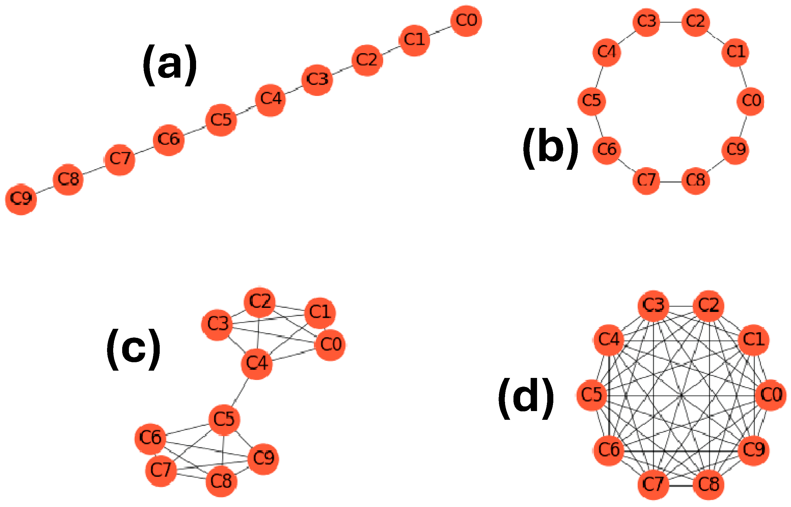
Further, since not all other ensemble members are required for the local clock’s correction, a host of different connection topologies can be envisioned for a timekeeping system (e.g., a satellite constellation). The local clock could connect to nearest neighbors in a straight chain, with end-clocks creating their correction based on one offset measurement as illustrated in Figure 2a; it could connect in a ring, with information passed along satellite crosslinks as in Figure 2b; it could connect in a barbell pattern as in Figure 2c, or in any other topology that suits the systems engineer.
Figure 2.
Illustrations of various connection topologies that could be implemented with the Kuramoto ensemble algorithm: (a) linear chain, (b) ring, (c) barbell, and (d) complete connections. In this regard, it is worth noting that there may be more than one stable equilibrium state for different topologies [17,18,19]. The clocks in each topologies are labelled with the letter “C” followed by an integer number.
Finally, and perhaps crucially important for the system engineer, the choice for clock steering is different in Kuramoto. In traditional ensemble methods, the ensemble member clocks must be statistically independent. This can be achieved by creating a paper clock that some (non-ensemble member) clock steers towards in order to create a realization of the ensemble timescale. It can also be achieved by creating a log of corrections for each ensemble member so that free-running histories can be created in software. In contrast, in Kuramoto the clocks are coupled through mutual steering so that each ensemble member is a physical representation of the timescale.
In the preliminary Kuramoto simulations, we use the power-law clock model, [20,21] combining white frequency noise (WHFM) and random walk frequency noise (RWFM) at levels measured for a commercial small-scale atomic clock, specifically the PRS-10 Rb clock from Stanford Research Systems (Sunnyvale, CA USA). Our motivation for employing this particular clock in our simulations is that it has been considered as a potential lunar satellite atomic clock [22]). Based on measurements made in our laboratory, we take and .
We use the two-state clock model following the work of Tavella [23,24], and then add the Kuramoto correction term. In the continuous case, the equations are as follows:
where is the Kuramoto correction term, is a numerical label for the clock, are the noise terms for phase and frequency, respectively, is the coupling strength between clock and , and are infinitesimal stochastic changes to the clock’s phase and frequency, respectively.
In order to study this set of Kuramoto stochastic differential equations, we simulated realizations using the following steps:
- Initialize the clocks’ states and define the clock connection topology (e.g., linear chain).
- Take the phase difference in each clock relative to its connected neighbors.
- Calculate the mean phase difference, assuming equal coupling parameters , at each node from each of its neighbors.
- Evolve each clock based on the sum of the clock’s internal state, a phase correction for each clock based on the results from step 3 and add new simulated noise.
- Repeat steps 2 through 4 until the final simulation time T is reached.
3. Results
3.1. MDEV of the Kuramoto Compared to EWFA and Free Running Clocks
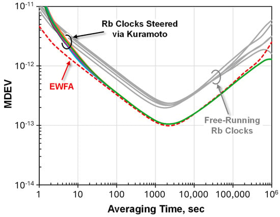
When the simulation is run for 107 s (computer simulation time) with a time step, , of one second, we obtain an MDEV as shown in Figure 3. The solid gray lines show the performance of the free-running simulated Rb clocks. To create some variability among the clocks, we vary each Rb clock’s WHFM and RWFM by multiplying their base noise level by a random number between 1 and 1.5. In addition, an initial time offset (uniformly distributed between −5 nsec and +5 nsec) is applied to the clocks. For averaging times less than a few seconds, we find each of the Kuramoto clocks (i.e., the Rb clocks steered by the Kuramoto algorithm) performs worse than any individual PRS-10. This is a result of applying a steering correction at each simulation interval [25]. However, after ~10 s there is clear improvement over the free running clocks. In addition, after ~100 s each clock in the Kuramoto ensemble performs comparably with EWFA, showing an improvement in frequency stability on the order of 1/√N where N is the number of clocks in the ensemble.
Figure 3.
Modified Allan deviation (MDEV) as a function of averaging time. The solid gray lines correspond to the MDEVs for the free-running Rb clocks, while the solid-colored lines correspond to the MDEVs of the Rb clocks (all five) steered by the Kuramoto algorithm. The dashed line is the MDEV from an Equal Weights Frequency Averaging (EWFA) ensemble algorithm for comparison. The Kuramoto algorithm simulated was a chain (see Figure 2a) with 5 clocks.
It is worthwhile to note that when plotting the MDEV performance, the choice of Kuramoto clock does not matter. In other words, as illustrated in Figure 3, the MDEV performance is replicated across all clocks in the ensemble, making each a realization of the improved clock performance. Compare this with more traditional timescale algorithms where the default output is a paper clock and extra work is needed to realize the paper clock (e.g., controlling the phase and/or frequency of a separate voltage-controlled crystal oscillator).
3.2. Time-Error Buildup
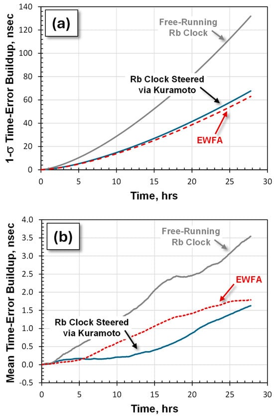
To estimate time-error buildup, we performed a Monte Carlo calculation, repeating the simulation 1500 times and computing the mean and variance of the time error for the Kuramoto algorithm. The results are shown in Figure 4. Figure 4a shows the 1-sided, 1-σ time-error level plotted as a function of time since synchronization. The gray line shows the time-error buildup for a free-running Rb clock, which performs two times worse than the Kuramoto and EWFA algorithms (only one Kuramoto-steered Rb clock is shown for clarity). In addition, the Kuramoto algorithm (solid blue line) and EWFA (dashed red line) perform about equally. In Figure 4b, we have the mean time-offset for the 1500 realizations. Without frequency drift, the free-running clocks and the EWFA and Kuramoto algorithms all have essentially the same mean time-error buildup in light of their 1 s levels: s >> Mean.
Figure 4.
(a) The standard deviation (1 s) time-error buildup as a function of time since synchronization. (b) The absolute value of the mean time-error buildup as a function of time since synchronization. Statistics were calculated from 1500 realizations of Monte Carlo simulations. The reader should note the difference in y-axis values between (a,b). These figures show that the Kuramoto time error is comparable to EWFA (a) and that the improvement in Kuramoto over a free-running clock cannot be attributed to a simple improvement of mean ensemble apparent drift (b).
3.3. Time to Achieve Kuramoto Synchronization
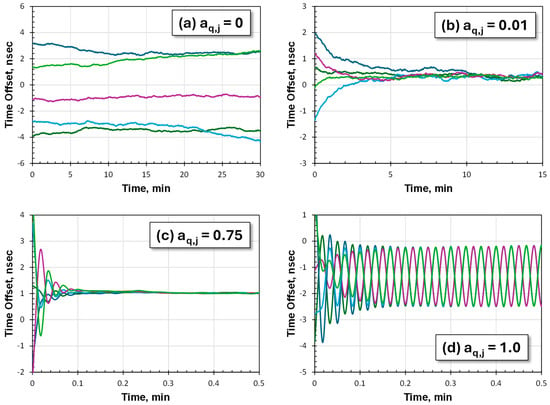
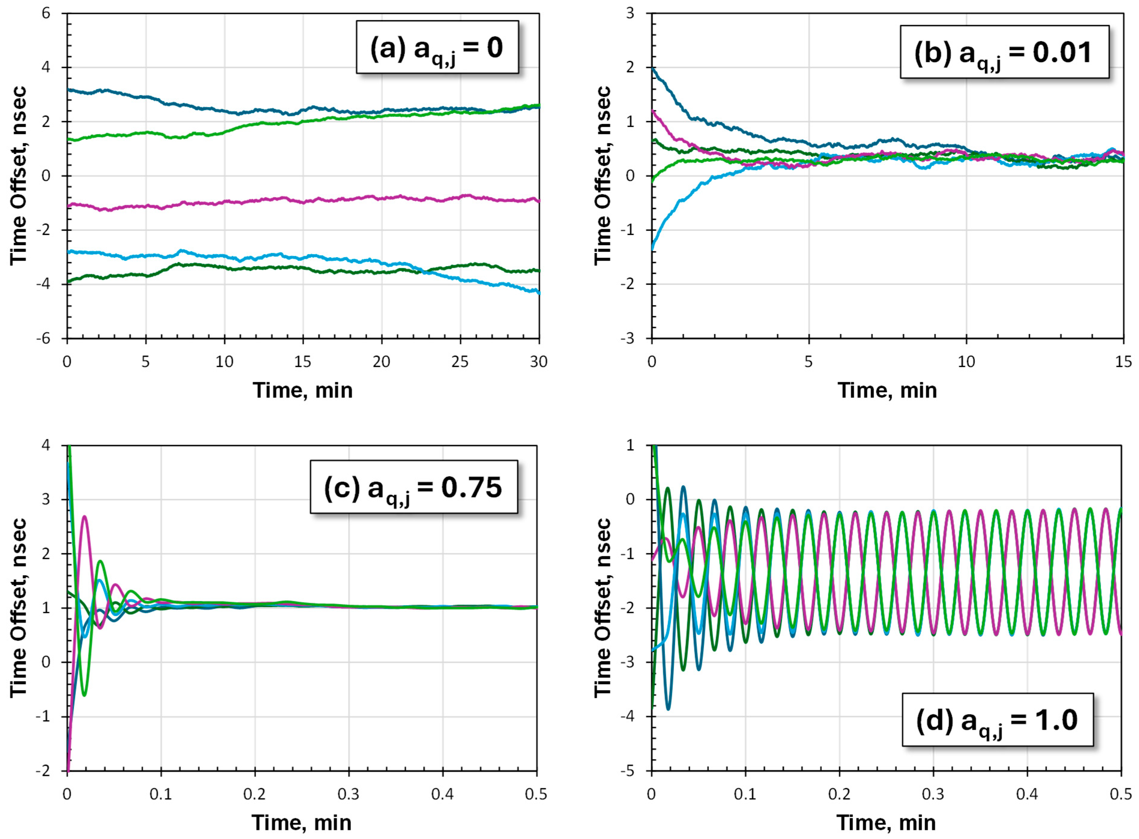
Here, we want to examine the effect of the coupling parameter (i.e., aq,j in Equation (1)) on the time to achieve synchronization for clocks initially offset from one another. Again, we performed 1500 Monte-Carlo runs, but this time with the goal of determining the relationship between the Kuramoto “loop attack time” and the Kuramoto coupling strength. Example realizations of the time offset among five simulated PRS-10 Rb clocks steered via the Kuramoto algorithm are shown in Figure 5a,d. When there is no coupling (aq,j = 0 ⟹ free-running clocks shown in Figure 5a), there is, not surprisingly, a persistent time offset among the clocks that only varies due to their individual stochastic frequency fluctuations. (We chose the initial time offset to be random and large relative to the clocks’ inherent stochastic fluctuations over 30 min.) In contrast, when we employ even a small coupling strength, the synchronization is achieved within the first ~10 min (Figure 5b). As the coupling strength increases, the time to synchronization (i.e., Kuramoto loop attack time) decreases. Not surprisingly, when the coupling strength becomes too strong, the Kuramoto algorithm becomes unstable, exhibiting oscillatory behavior, as shown in Figure 5d. One way to interpret this result is that the clock correction terms become of similar magnitude to an individual clock’s noise. This will lead to an overcorrection, thereby driving oscillations.
Figure 5.
Time to synchronization for five simulated PRS-10 Rb clocks (different colors) steered via the Kuramoto algorithm with an open chain (Figure 2a), considering several different Kuramoto coupling strengths: (a) ai,j = 0, (b) ai,j = 0.01, (c) ai,j = 0.7, and (d) ai,j = 1.0.
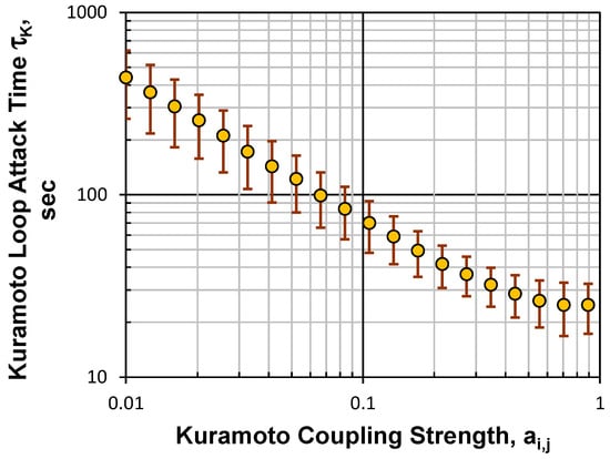
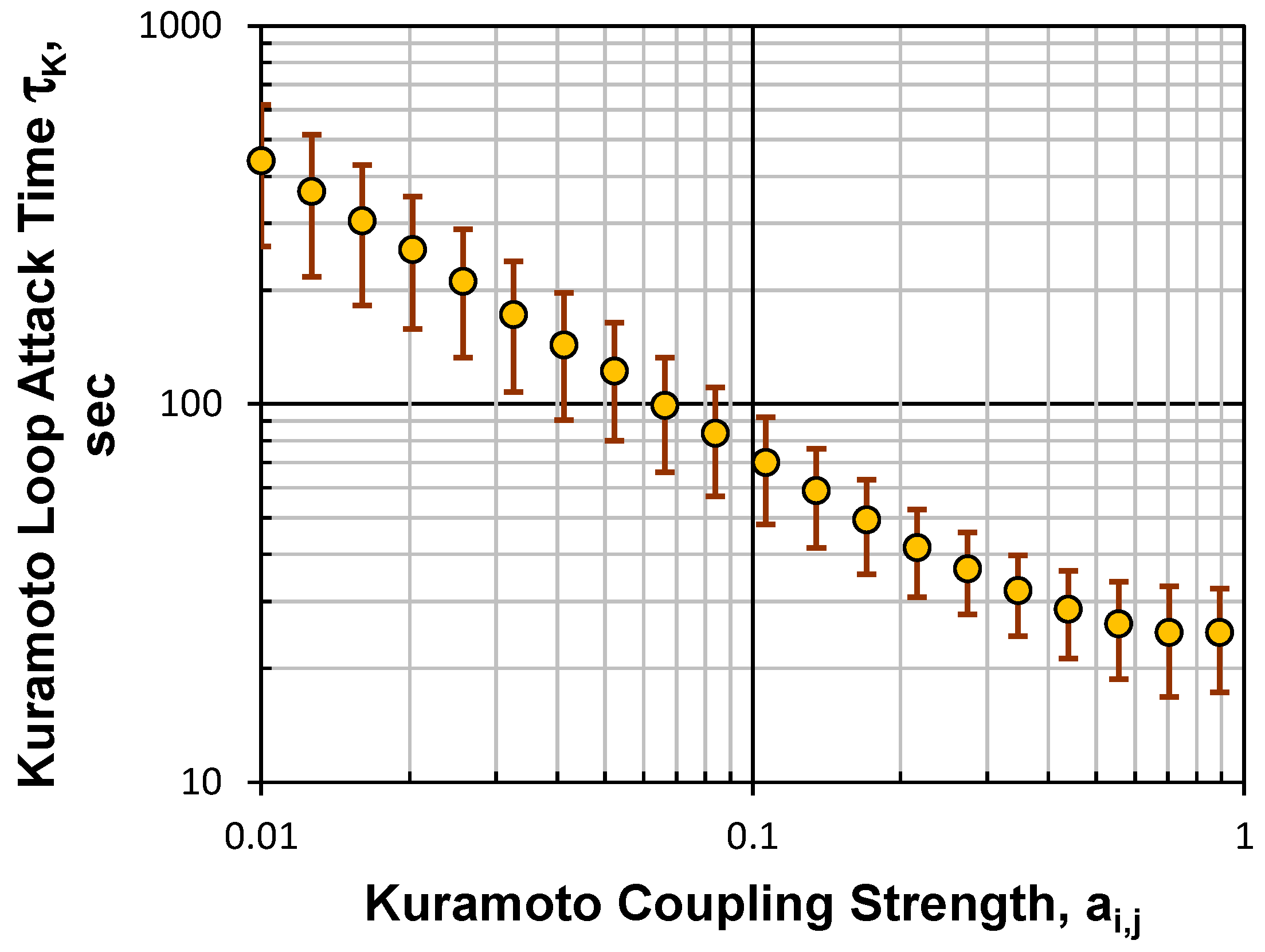
In Figure 6, we plot the Kuramoto loop attack time tK as a function of the Kuramoto coupling strengths aq,j. We define the Kuramoto loop attack time as the time interval from t = 0 to the time when the (time-error) standard deviation of the 5-clock Kuramoto ensemble is equal to or less than the EWFA algorithm’s Time Interval Error (TIE):
Figure 6.
Kuramoto loop attack time as a function of the Kuramoto coupling strength for linear chain of five clocks as in Figure 2a. For weak coupling the Kuramoto loop attack time is large and in a few cases never synchronizes. As the coupling strength increases the Kuramoto loop attack time decreases along with the standard deviation of the loop attack time.
The TIE for EWFA was found using separate simulations. In our assessment of the Kuramoto loop attack time, if Equation (6) was not met within the first 105 s of computer simulation time, the loop attack time was set to NaN. This guarded against those initial conditions or coupling strengths that could lead to Kuramoto instability. For the coupling strengths chosen, all simulations resulted in synchronized behavior. After the 1500 simulations, the mean and standard deviation were computed. For small coupling parameters, the time to synchronization is expectedly longer, and as one might expect, the variance of synchronization times is greater (i.e., the corrections are weak and only poorly able to overcome the myriad stochastic phase variations). When the coupling parameter is increased, the time to synchronization becomes shorter, as does the variance of Kuramoto loop attack times (i.e., the corrections are large and easily able to overcome the myriad stochastic phase variations).
3.4. Simulation of an Operational Environment: Constellation Fragmentation/Defragmentation
In this section, we consider a constellation of satellites, perhaps lunar-orbiting satellites, that are connected and sharing timing information via crosslinks. At some point in time, one set of crosslinks “goes down” fragmenting the constellation. At a later point in time, through autonomous constellation procedures, the crosslinks are re-established, and the constellation defragments. The question we address here concerns the ability of the Kuramoto algorithm to deal with constellation defragmentation. (Constellation fragmentation is of no such concern, since the two fragments would simply form two separate Kuramoto timescales.)
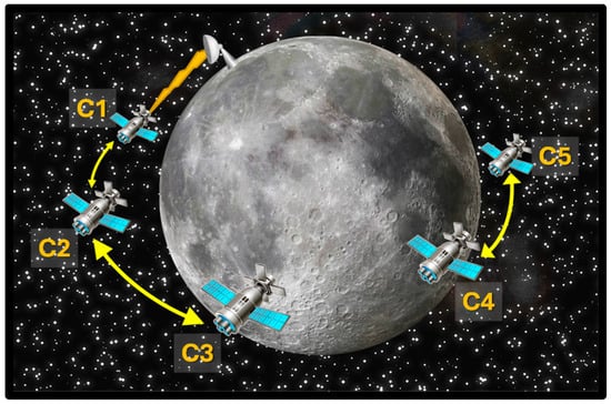
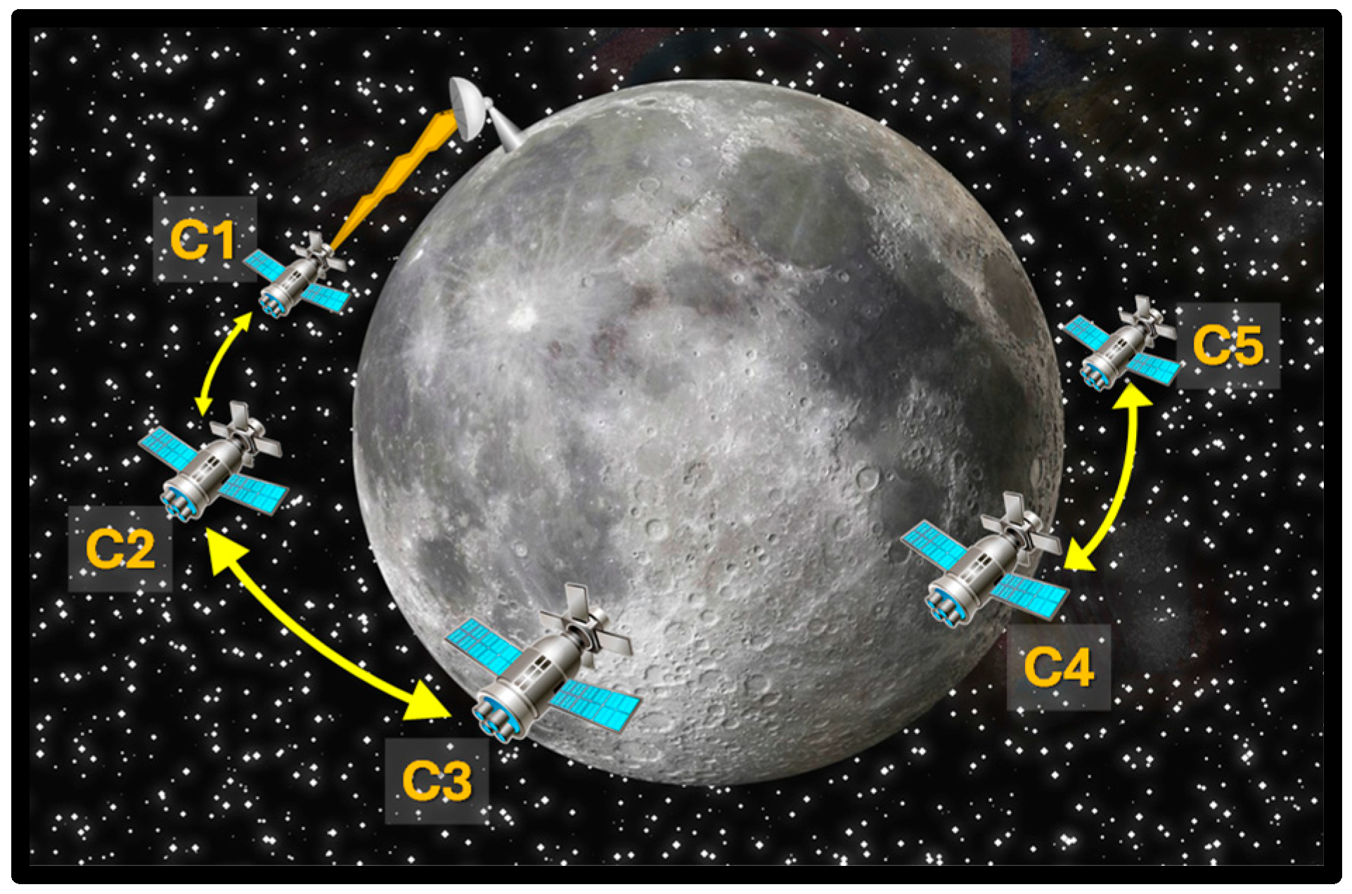
For our first simulation, we considered a scenario where a reference lunar-ground clock was connected to one end of a chain of satellite clocks (call this satellite clock Clock-C1), and our starting condition was a fragmented constellation: three satellite clocks in one fragment and two in the other fragment, as illustrated in Figure 7. Again, we consider the satellites to be carrying small Rb clocks similar to the SRS PRS-10, and for the ground-station clock, we consider a device with performance similar to a cold-Rb clock (SpectraDynamics Inc, Louisville, CO, USA) [26].
Figure 7.
Pictorial representation of a fragmented lunar satellite constellation (all images are Creative Commons.). C1–C5 are labels for the clocks and the arrows represent the connections between clocks.
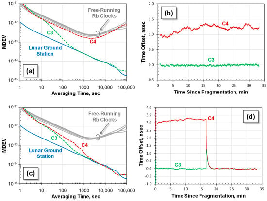
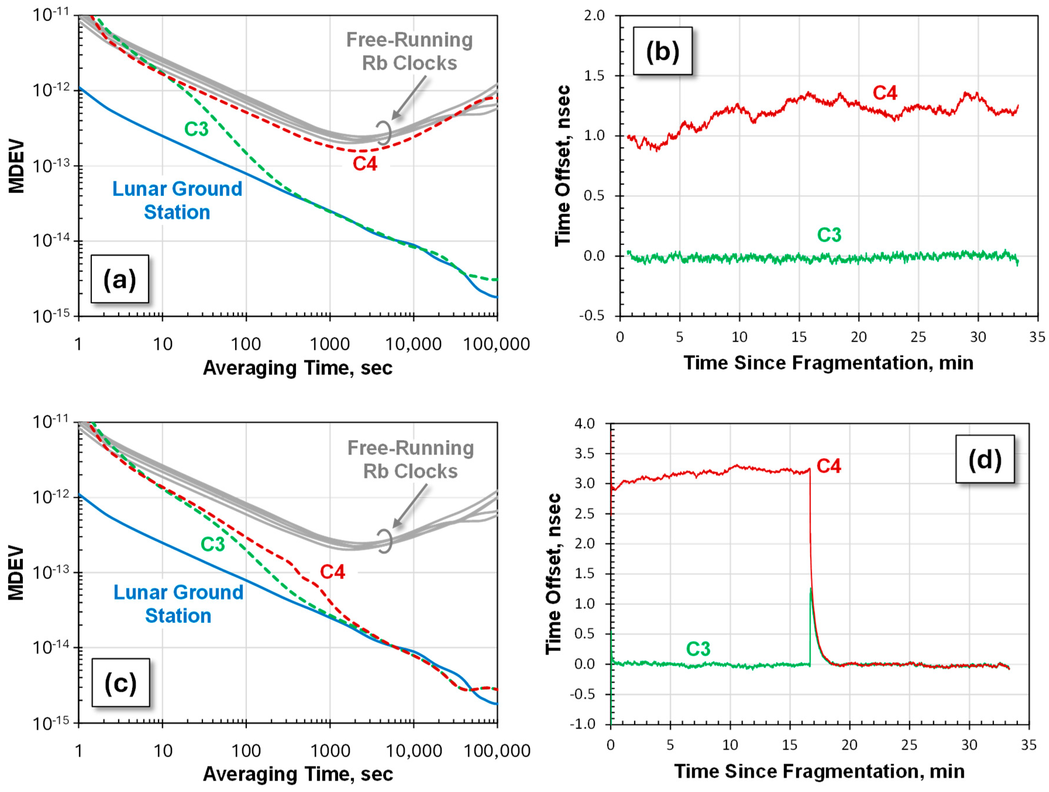
The ground-station (i.e., reference) clock sends its phase to C1 but does not update its phase or frequency with the Kuramoto algorithm. C4 and C5 are connected via their own internal Kuramoto algorithm but fragmented from C1–C3. In the first simulation, we examined the performance when the two subsets are initially fragmented and stay fragmented. The Kuramoto clocks that are attached to the lunar-ground reference clock initially follow the performance of a free-running PRS-10 but start to follow the performance of the reference clock at ~300 s, as seen in Figure 8a. In addition, the fragmented Kuramoto clocks (C4 and C5) follow each other’s phase but drift from the reference-clock ensemble. The performance of the fragment disconnected from the lunar ground station predictably performs 1/√2 better than an individual free-running PRS-10, but poorer than the ground-station clock.
Figure 8.
Examination of defragmentation for a lunar constellation of satellites. In all cases, the Kuramoto coupling strength is 0.75. (a) The MDEV of the constellation with clocks from each Kuramoto fragment shown as dashed lines. (b) Two individual realizations of the Kuramoto clocks: C3 and C4. (c) MDEV of the same system but the fragmented clocks are now defragmented after about 15 min. Following defragmentation and after a few hundred seconds of averaging time, the MDEV performance of all spacecraft clocks is similar to the ground-station clock. (d) Two individual realizations of the Kuramoto clocks in the fragmentation/defragmentation simulation. After about 15 min the entire 5-clock constellation synchronizes via the Kuramoto algorithm.
In the second simulation, the two chains are initially fragmented, but after about 15 min it is assumed that all crosslinks are re-established and the constellation defragments. All clocks then begin to synchronize to the lunar ground station via the Kuramoto algorithm, and very shortly all clocks are tightly synchronized to the ground-station clock (i.e., Figure 8c,d). This simulation illustrates how the Kuramoto ensemble algorithm would perform under realistic operational conditions when satellite crosslinks might be broken and then reestablished.
4. Discussion
Within the next ten years, manned lunar exploration will be a reality, and by the end of the century, manned Martian exploration could be a reality as well. All of this focuses attention on the importance of accurate PNT within the inner solar system. As noted in the Introduction, one of the major technical challenges to this goal will be achieving an accurate and stable timescale employing low-SWaP atomic clocks, and the most direct path forward will be to create lunar-orbiting and Mars-orbiting satellite clock ensembles. Since the satellites will likely be small and could be extensive in number, this would place a connectivity and computational burden on the satellites if they were to employ presently established ensemble algorithms.
To solve this problem, we have introduced here the concept of a Kuramoto ensemble timescale. We showed how this could allow greater flexibility in constellation connection topologies and how it could simplify the information any one satellite would need in order to create the ensemble timescale. We showed that in its simplest form, its stability was equivalent to an Equal Weights Frequency Averaging (EWFA) ensemble algorithm, and that it could deal seamlessly with situations of constellation fragmentation and defragmentation.
In future work, we plan to explore the ability to create a Kuramoto ensemble timescale using frequency (as opposed to phase) corrections, to include dynamic weights to Kuramoto ensemble members, to test the algorithm with clocks of widely varying characteristics, and to account for data latency effects in crosslink transmissions. In addition, it will be important to understand how the Kuramoto algorithm needs to be modified in order to deal with clock anomalies and clock failures, how Kuramoto responds to space dynamics (e.g., relativity), and how the algorithm responds to dynamically changing clock-connection topologies. Notwithstanding the work that remains, the Kuramoto ensemble timescale appears to be a very promising path for achieving accurate and stable timekeeping throughout the inner solar system. Consequently, in answer to the question first posed in the Introduction: YES, the community of precise timekeeping metrologists has reason to explore (and should explore) the Kuramoto concept for precise timekeeping further.
5. Patents
The Aerospace Corporation has a patent pending regarding the Kuramoto concept for precise timekeeping.
Author Contributions
Conceptualization, N.R., H.K. and J.C.; methodology, N.R., H.K. and J.C.; software, N.R. and H.K.; validation, N.R., H.K. and J.C.; formal analysis, N.R., H.K. and J.C.: investigation, N.R. and H.K.; resources, N.R., H.K. and J.C.; data curation, N.R. and H.K.; writing—original draft preparation, N.R. and J.C.; writing—review and editing, N.R., H.K., and J.C.; visualization, J.C.; supervision, J.C.; project administration, N.R.; funding acquisition, N.R., H.K. and J.C. All authors have read and agreed to the published version of the manuscript.
Funding
This work was funded by the Aerospace Corporation’s Internal Research and Development (IRaD) funding.
Data Availability Statement
Data is available under certain restricted conditions based on corporate policy.
Acknowledgments
The authors thank Michael Huang, Eliott Bergerson, and Daniele Monahan for their helpful insights and discussions.
Conflicts of Interest
N.R., H.K. and J.C. are employed by Aerospace Corporation. All authors declare no conflicts of interest. The funders had no role in the design of the study; in the collection, analysis, or interpretation of the data; in the writing of the manuscript; or in the decision to publish the results.
Abbreviations
The following abbreviations are used in this manuscript:
| SWaP | Size, weight and power |
| pLEO | Proliferated low earth orbit |
| EWFA | Equal weights frequency averaging |
| PNT | Position, navigation and timing |
| MDEV | Modified Allan deviation |
| TIE | Time interval error |
References
- Gramling, C.; Crenshaw, J.; Mann, L. Interoperable Services to Mitigate Lunar Position, Navigation, and Timing Challenges. In Proceedings of the 73rd International Astronautical Congress, Paris, France, 18–22 September 2022. [Google Scholar]
- Greenhall, C. A Review of Reduced Kalman Filters for Clock Ensembles. IEEE Trans. Ultrason. Ferroelectronics Freq. Control. 2012, 59, 491–496. [Google Scholar] [CrossRef] [PubMed]
- Wang, Q.; Rochat, P. ONCLE (One Clock Ensemble) for Galileo’s Next-Generation Robust Timing System. Navigation 2022, 69, navi.536. [Google Scholar] [CrossRef] [Scilit]
- Yan, Y. Structured Kalman Filter for Time Scale Generation in Atomic Clock Ensembles. IEEE Control. Syst. Lett. 2024, 8, 187–192. [Google Scholar] [CrossRef] [Scilit]
- Weiss, M.; Weissert, T. AT2, A New Time Scale Algorithm: AT1 Plus Frequency Variance. Metrologia 1991, 28, 65–74. [Google Scholar] [CrossRef] [Scilit]
- Bauch, A.; Staliuniene, E.; Gomah, G. A status report on time scale generation at PTB. In Proceedings of the 2015 Joint Conference of the IEEE International Frequency Control Symposium & the European Frequency and Time Forum, Denver, CO, USA, 12–16 April 2015. [Google Scholar]
- Camparo, J.; Driskell, T. A master/slave “ensembling” procedure for satellite-system timekeeping. In Proceedings of the 51st Annual Precise Time and Time Interval Systems and Applications Meeting, San Diego, CA, USA, 21–24 January 2020; Institute of Navigation: Manassas, VA, USA, 2020; pp. 302–309. [Google Scholar]
- Kuramoto, Y. Self-Entrainment of a Population of Coupled Non-Linear Oscillators; Araki, H., Ed.; Lecture Notes in Physics: Kyoto, Japan, 1975; Volume 39. [Google Scholar]
- Strogatz, S.H. From Kuramoto to Crawford: Exploring the onset of synchronization in populations of coupled oscillators. Phys. D Nonlinear Phenom. 2000, 143, 1–20. [Google Scholar] [CrossRef] [Scilit]
- Acebrón, J.A.; Bonilla, L.L.; Vicente, C.J.P.; Ritort, F.; Spigler, R. The Kuramoto model: A simple paradigm for synchronization phenomena. Rev. Mod. Phys. 2005, 77, 137–185. [Google Scholar] [CrossRef] [Scilit]
- Buck, J. Synchronous Rhythmic Flashing of Fireflies. II. Q. Rev. Biol. 1989, 63, 265–289. [Google Scholar] [CrossRef] [Scilit] [PubMed]
- Ermentrout, B. An adaptive model for synchrony in the firefly Pteroptyx malaccae. J. Math. Biol. 1991, 29, 571–585. [Google Scholar] [CrossRef] [Scilit]
- Chauhan, K.; Khaledi-Nasab, A.; Neiman, A.B.; Tass, P.A. Dynamics of phase oscillator networks with synaptic weight and structural plasticity. Sci. Rep. 2022, 12, 15003. [Google Scholar] [CrossRef] [Scilit] [PubMed]
- Lucken, L.; Popovych, O.V.; Tass, P.A.; Yanchuk, S. Noise-enhanced coupling between two oscillators with long-term plasticity. Phys. Rev. E 2016, 93, 032210. [Google Scholar] [CrossRef] [Scilit] [PubMed]
- Ulrichs, H.; Mann, A.; Parlitz, U. Synchronization and chaotic dynamics of coupled mechanical metronomes. Chaos 2009, 19, 043120. [Google Scholar] [CrossRef] [Scilit] [PubMed]
- Pantaleone, J. Synchronization of metronomes. Am. J. Phys. 2002, 70, 992–1000. [Google Scholar] [CrossRef] [Scilit]
- Girnyk, T.; Hasler, M.; Maistrenko, U. Multistability of twisted states in non-locally coupled Kuramoto-type models. Chaos 2012, 22, 013114. [Google Scholar] [CrossRef] [Scilit] [PubMed]
- Townsend, A.; Stillman, M.; Strogatz, S.H. Dense networks that do not synchronize and sparse ones that do. Chaos 2020, 30, 083142. [Google Scholar] [CrossRef] [Scilit] [PubMed]
- Aoki, T.; Aoyagi, T. Co-evolution of Phases and Connection Strengths in a Network of Phase Oscillators. Phys. Rev. Lett. 2009, 102, 034101. [Google Scholar] [CrossRef] [Scilit] [PubMed]
- Ashby, N. Confidence Estimates in Simulation of Phase Noise or Spectral Density. IEEE Trans. Ultrason. Ferroelectr. Freq. Control. 2017, 64, 872–878. [Google Scholar] [CrossRef] [Scilit] [PubMed]
- Hutsell, S.T. Fine Tuning GPS Clock Estimation in the MCS. In Proceedings of the 26th Annual Precise Time and Time Interval Systems and Applications Meeting, Reston, VA, USA, 6–8 December 1994. [Google Scholar]
- Bhamidipati, S.; Mina, T.; Gao, G. A Case Study Analysis for Designing a Lunar Navigation Satellite System with Time Transfer from the Earth GPS. Navigation 2023, 70. [Google Scholar] [CrossRef] [Scilit]
- Zucca, C. The Clock Model and Its Relationship with Allan and Related Variances. IEEE Trans. Ultrason. Ferroelectr. Freq. Control. 2005, 52, 289–296. [Google Scholar] [CrossRef] [Scilit] [PubMed]
- Tavella, P. Statistical and mathematical tools for atomic clocks. Metrologia 2008, 45, 183–192. [Google Scholar] [CrossRef] [Scilit]
- Schmidt, T.; Trainotti, C.; Furthner, J. Comparing clock steering technique performances in simulations and measurements. In Proceedings of the 50th Annual Precise Time and Time Interval Systems and Applications Meeting, Reston, VA, USA, 28–31 January 2019. [Google Scholar]
- Ascarrunz, F.; Dudin, Y.; Delgado Armburo, M.; Ascarrunz, L.; Savory, J.; Banducci, A. A Portable Cold 87Rb Atomic Clock with Frequency Instability at One Day in the 10−15 Range. In Proceedings of the 2018 IEEE International Frequency Control Symposium, Olympic Valley, CA, USA, 21–24 May 2018. [Google Scholar]
Disclaimer/Publisher’s Note: The statements, opinions and data contained in all publications are solely those of the individual author(s) and contributor(s) and not of MDPI and/or the editor(s). MDPI and/or the editor(s) disclaim responsibility for any injury to people or property resulting from any ideas, methods, instructions or products referred to in the content. |
© 2026 by the authors. Licensee MDPI, Basel, Switzerland. This article is an open access article distributed under the terms and conditions of the Creative Commons Attribution (CC BY) license.