
Commodity and Equity Markets: Volatility and Return Spillovers


1
GOVCOPP—Unidade de Investigação em Governança, Competitividade e Políticas Públicas DEGEIT, Departamento de Economia, Gestão, Engenharia Industrial e Turismo, Universidade de Aveiro, 3810-193 Aveiro, Portugal
2
REMIT—Research on Economics, Management and Information Technologie, Universidade Portucalense, 4200-072 Porto, Portugal
*
Author to whom correspondence should be addressed.
Commodities 2022, 1(1), 18-33; https://doi.org/10.3390/commodities1010003
Submission received: 24 May 2022
/
Revised: 11 July 2022
/
Accepted: 15 July 2022
/
Published: 19 July 2022
Abstract
:The present paper provides an empirical analysis of the relationship between shocks to commodity markets and stock markets. By employing a total volatility connectedness measure, we study the relationship between shocks to oil, gold, copper, and agricultural commodity markets and emerging and developed stock markets. We conduct a connectivity analysis in the time and frequency domain to quantify market linkages using volatility spillovers over the period from 2004 to 2021. In addition, we analyze the spillovers of returns in these markets over the same period. The results suggest that both on volatility and returns spillovers, slightly more than 35% of the total variance of forecast errors is explained by shocks to markets during the period January 2004 to June 2021. We also show that, in terms of both volatility and returns, the contribution of equity market shocks to other markets is substantially more important than that of commodities; however, our analysis reveals that the total link between market returns is larger in the short run than in the long run, while in the case of volatility, the long-run frequencies concentrate the market link. Additionally, we use dynamic analysis to assess both the time evolution of total connectivity and all directional partial connectivity between markets. Our results show that both volatility and return linkages change significantly over time and that a set of events has a significant impact on them.
1. Introduction
The increasing importance of commodities for financial investors observed over the last few decades, a period in which significant capital inflows have been directed to commodity markets, has raised new questions that a large number of researchers have been addressing.
From the beginning of commodity financialization, with increased integration of stock and commodity markets worldwide, the effects of this process on price levels, returns, and volatilities have been the subject of debate.
Despite the increasing degree of market integration, with a potential effect on the similarity of price trajectories and market volatilities, the risk and return level in each market still appears to be different.
The aim of this paper is to conduct an analysis of the return and volatility linkages between four major commodity markets and financial markets. We empirically examine the dynamics of returns and volatility connectedness, and spillover transmission in five major commodity markets and two worldwide stock indices. Using a daily dataset from January 2004 to June 2021, this study presents the static and dynamic quantification of market connectedness using return and volatility spillovers in emerging stock markets, developed stock markets, oil, copper, soybean, corn, and gold markets, based on a connectedness measure for gauging the dependencies and effects of spillovers.
Financial deregulation, the development of new and widespread information technologies, and the emergence of financial innovations are among the main factors that in recent decades have significantly contributed to a highly connected financial system with significant increases in the level of integration and interdependence of financial and commodity markets. In such integrated markets and with the surge of stress periods, such as the global financial crisis or a pandemic crisis, even with different economic fundamentals, the propensity for risks in one market to spillover to other markets increases considerably. The combination of linkages arising from fundamental channels between markets and behavioural channels has led to important contagion effects.
Many studies have discussed the dynamic interrelationships among commodities markets, or between several commodities and financial markets with special incidence on energy and/or precious metals markets and equity markets, with the main focus on the dynamic and level of spillovers effects. Under the alternative approach, the main objective of this study is to expand upon the literature on spillovers and connectedness among markets by exploring not only the intensity but also the directional dynamic spillover effects and connectedness for both return and volatility at time and frequency domains of developed and emerging equity markets and major commodity markets. With our approach, we analyse the dynamic cycle connectedness of equity and commodity markets over an extended period of time, identifying which markets play a relevant role as receivers and transmitters of return spillovers and volatility spillovers and how this role shifts over time.
The main contributions of the paper can be summarised as follows. First, in this study, we look together at volatility and return spillovers in agricultural, industrial, precious metals, and equity markets with a systemic approach over almost two decades. Second, we use time and frequency analysis to study connectedness over commodity and equity markets looking at both emerging market and developed equity markets. Third, we conduct dynamic analysis in order to identify the recipients and transmitters of risks across markets over the large period analysed.
Overall, our results suggest that commodity markets are net recipients rather than net transmitters of spillovers to equity markets, although several shifts have occurred over time, with a significant number of events affecting the level and direction of spillovers.
The total spillover shows almost the same connectedness dimension measured by returns or by volatility, but the returns spillovers are concentrated at high frequencies (short term), while the volatility spillovers are concentrated at the low frequency (long-term).
Agricultural markets are the most neutral in the network with small spillovers to and from the system. The energy (oil) and industrial (copper) markets are net receivers of volatility spillovers from the system with important incidence following several major events such as the global financial crisis, the European debt crisis, or the beginning of the COVID-19 crisis. Analysis of the pairwise network connectedness shows gold as an important net receiver of equity market shocks most of the time.
2. Literature Review
Over the past decades, new questions have been raised about financial and commodity markets, as important capital flows have been directed to the commodity market by financial investors and as these markets have been seen by investors as a way to diversify their portfolios.
A large body of literature has addressed some of these questions, using a wide variety of methodological approaches, modelling the volatility, analysing interdependencies, volatility and return spillovers, dynamic linkages, contagion effects, and co-movement effects are some of the issues widely explored recently.
One group of empirical studies has been directed toward modelling and forecasting commodity volatility as an important issue in asset allocation, asset pricing, and financial risk management (see, among others, [1,2,3,4,5,6,7,8]). A considerable number of these studies have examined the predictive power of distinctive volatility measures, using conditional volatility, such as GARCH family models [2,4] or realized volatility (RV) [1,3].
On the other hand, a significant part of the research focuses on the time-varying relationship between commodity markets, and between commodity and stock markets; this research has largely been centred on the relationship between oil and the financial markets. Authors, such as [9,10,11,12] used the Dynamic Conditional Correlation approach to find that the relationship between stock markets and oil prices is time-varying. The direction of this impact in both oil-importing and oil-exporting countries shifted during the global financial crisis. Ref. [9] estimated the volatility spillover effect among the stock equity market and several commodity markets, copper, wheat, and oil prices, also by applying the multivariate GARCH models and showing that conditional correlations present considerable variability across the sample period analysed. Ref. [13] study the interdependence of returns, volatilities, and correlations across the S&P 500, beverage, wheat, gold, Brent, and WTI. The paper based on the VAR-GARCH model shows the presence of significant evidence of volatility transmission of the equity markets to the gold and oil markets. More recently, [14] examine the volatility spillover between oil and three emerging stock markets by using the bivariate BEKK-GARCH model and conclude that there exists a spillover between oil and stock markets and vary across crisis periods. All these studies conclude that volatility spillover varies over time, being higher during turbulent periods, such as financial crises.
Another group of studies explores the nonlinear connections between classes of assets at the time and frequency domains by analyzing the connections of the prices at different periodicities and at different moments in time. In this group of studies, we have [15,16,17].
Ref. [16] using wavelet decomposition and time-varying copulas analyse the S&P500, EURO STOXX, crude oil, heating oil, natural gas, copper, platinum, gold, silver, and palladium prices, and show that the dependence between stock returns and commodities appears to be weak, yet they are characterized by a strong long-run dependence.
Recently, a growing number of studies based on Diebold and Yilmaz’s framework, ([18,19]), focused on quantitative measures of the direction and size of spillovers; these studies have been analyzing spillovers across different asset classes, such as oil, exchange rates, stock prices, cryptocurrencies, and precious metals (see, among others, [20,21,22,23,24,25,26,27,28]).
Ref. [21] analyzed the directional connectedness between the oil implied volatility and the implied volatility of equities in eleven major equity markets from 2008 to 2015. The results indicated volatility transmissions from the oil market to equity markets; however, [26] applied connectedness measures to study the return and volatility spillovers among S&P 500, crude oil, and gold and reported a bidirectional return and volatility spillover among these assets. Ref. [25] present results from return connectedness among stock, currency, bond, and commodity markets from December 1999 to June 2016, and conclude that net spillover shock transmission is dominated by the US stock market and the oil market is neutral to the network, while the gold market is a net recipient of return spillover shocks.
Ref. [28] study the connectedness across U.S. sector equity ETFs, oil, gold, stock markets, and uncertainty measures and their results show the strong effect of oil and volatility indexes (VIX and OVX) on US sector equity ETFs in the short and long term; conversely, gold has a weak effect.
In summary, although the relevance of analysing returns and volatility spillovers across major commodity and stock markets, the existing literature seems to be inconclusive. To address this caveat in the existing literature, this paper analyses the network comprising four commodity markets and two equity indices. Our focus is on both return and volatility spillover effects examining the dynamic time-frequency dependence and connectedness structure among industrial, agricultural, precious metals, and energy commodities, and developed and emerging financial markets.
3. Methodology
The core method used in this paper is essentially a multivariate time-series approach developed by [18]; they introduce a simple measure of connectedness to explicitly account for interdependence in financial markets; this measure is then used to look at spillover effects in the global financial market as it has been shown to be a very simple but successful idea.
This method has been widely expanded to study systems in many areas of the economy. The methodology is based on the vector autoregressive process (VAR) and the use of forecast error variance decomposition (FEVD) to estimate the connectedness.
Consider an N variable VAR (p) model in the form
The moving average representation of VAR(p) is
The H-step-ahead forecast error variance decomposition
where is a vector equal to one as i-th element and zeros otherwise, is the standard deviation of the forecast error term, and is the variance matrix for the error vector .
In order to bound the spillover index between zero and one, [19] standardize the variance decomposition by:
The connectedness measure is then given by:
To show the influence of one variable on the system connectedness, or the volatility spillover from the variable i to all other variables j, we have
The directional spillover received by market i from all other markets j
The net directional connectedness (NDC) is the difference between the shocks transmitted to all other markets and received from all other markets:
Next, following [29], we discuss the frequency dynamics of the connectedness and describe the spectral formulation of variance decomposing.
Hence, we consider a frequency response function, , which we can obtain as a Fourier transform of the coefficients Ψ, with .
The generalized causation spectrum over frequencies is
where is the Fourier transform of the impulse response function and denotes the portion of the spectrum of the j-th variable under frequency ω due to shocks in the kth variable.
As the denominator holds the spectrum of the j-th variable under frequency ω, we can interpret Equation (9) as the quantity within the frequency causation.
To obtain the generalized decomposition of variance decompositions under frequency ω, we weight the function by the frequency share of the variance of the j-th variable.
We can define the weighting function as in Equation (9):
Equation (10) shows the power of the j-th variable under frequency ω, and the sums of the frequencies to a constant value of 2π.
We should note that although the Fourier transform of the impulse response is a complex number value, the generalized factor spectrum is the squared coefficients of the weighted complex numbers, and hence a real number. Formally, we begin to set up frequency band d = (a, b): a, b ∈ (−π, π), a < b.
The generalized variance decomposition under the frequency band d is
It is relatively easy to formulate the connectedness measures under the frequency band using the spectral formulation of the generalized variance decomposition.
We formulate the scaled generalized variance decomposition under the frequency band d = (a, b): a, b ∈ (−π, π), a < b as
We can formulate the within connectedness under the frequency band d as:
Next, we can formulate the frequency connectedness under the frequency band d as:
4. Data and Preliminary Analysis
Our study was based on daily frequency data on five futures markets and two equity indices for the period 5 January 2014 to 30 June 2021 on a total of 4359 business days.
We use a sample of Chicago Board of Trade (CBOT) corn (C1) and soybeans (S1) futures, New York Metal Exchange (NYMEX) WTI crude oil (CL1) futures and Commodity Exchange Inc. (COMEX) gold (GC1) and copper (HG1). The Morgan Stanley Capital International (MSCI) Emerging Markets Index (EEM) is the index that measures the equity market performance in global emerging markets and the MSCI EAFE Index (EFA) measures the equity market performance of developed markets outside of the U.S.
The data were transformed into log returns of stock market indices and prices and the series corresponding to the conditional volatility are based on AR(1)-GARCH(1,1) model for all series as follows.
Consider , the log-return of the price series is given by
where
and the conditional variance of is given by
In line with the literature, we decided transform all volatility series into their natural logarithm as the transformed series conform more closely to normal distribution than the original series.
Table 1 presents the descriptive statistics of the conditional volatility indices as well as of the logarithmically transformed series. Among all volatility indices, oil shows the highest mean and the highest standard deviation, while gold shows the lowest mean and the lowest standard deviation. Over the whole sample, oil investors seem to be clearly the most worried about the price variability expressed not only with its highest mean but also with the highest minimum, maximum and standard deviation. All volatility series show evidence of leptokurtic distribution as evidenced by the measures of skewness and kurtosis, and the Jarque–Bera test statistic, so we can reject the normal distribution hypothesis for all series. The high values of kurtosis estimates suggest the presence of extreme fluctuations.
To ensure that all the series included in the VAR framework are stationary, an Augmented Dickey–Fuller (ADF) test is employed, and the results for all series are far less than critical values at 5% significance levels, thus evidencing that there is no unit root in the sample series, and they are stationary time series.
Table 2 presents the correlation coefficient between the variables. Panel B presents the volatility case. All coefficients are positive and highly significant; they show a higher correlation between the equity markets as well as between each of the equity markets with the gold market. On the opposite side, the correlations between the oil market and agricultural markets are rather low. In the other cases, in general, the correlation values are moderately positive.
Correlations between equity return markets are very high but their relationship with other markets, particularly with copper and gold, are much weaker than those exhibited by volatility.
5. Empirical Results
5.1. Full-Sample Spillover Analysis
Table 3 reports the full-sample connectedness results of a variance decomposition based on seven return and volatility series VAR. Bayesian Information Criteria (BIC) are used to choose lag length. All results are based on vector autoregressions and generalized variance decompositions of 100-day ahead volatility forecast errors.
Table 4 and Table 5 show the connectedness results for returns and volatility, respectively, when we decompose the series into three frequencies which are shown in Panel A to Panel C. The frequencies correspond to a time frame of 1 to 5 days—short-term, 5 to 21 days—medium-term—and the long-term frequency corresponds to more than 21 days.
The amount of spillover effects in this variable VAR system, measured by the total connectedness of volatilities, is around 36.81% and the connectedness of returns is 35.43%, i.e., according to these results 63.17% and 64.5% of the variation of volatility and returns respectively, is due to idiosyncratic shocks.
Although the figures for the total connectedness of the volatility and returns system are very close, there are important differences between them. Over the period, the commodities’ volatility responds more to shocks received from the system than their shocks contribute to. The same conclusion can be achieved from the connectedness analysis of returns, with rather lower importance of equity market shocks to commodities.
Over the analysis period, 2014–2021, all commodities respond more to the shocks received from the system than their shocks contribute to them. The oil volatility contributes only 5.53% to the total variation in the system and the system contributes 17.8% to the oil volatility with returns the contribution of oil shocks is 20.84% and the system contribution shocks to oil is 25.56%. The same pattern of negative net connectedness relative to the system can be observed for all other commodities, using volatility and returns, with special importance for copper and gold at volatility analysis and gold and oil for returns spillovers.
Agricultural commodities show an almost neutral spillover contribution to markets other than agricultural commodity markets.
The equity markets contribute to on average 87.25% and receive on average 40.5% from the volatility system and contribute to on average 57.02% and receive on average 51.2% from the returns system, so they are net contributors.
Figure 1 shows how the system is connected variable to variable. An arrow from variable i to variable j correspond to a net directional connectedness between the indices. Red line arrows connect system members with the highest total net directional connectedness, whereas blue and grey line arrows connect the lowest total net directional connectedness.
The commodities markets are net receivers of shocks from each other’s and mainly from stock markets. Stock markets contribute more than they receive from all other markets; this result can be seen as evidence of a high level of impact of equity markets on commodity markets.
The spillover results based on frequencies, presented in Table 4 and Table 5, show the short-, medium-, and long-term spillovers in the markets, classified into three frequency bands (intraweek, week-to-month, beyond month), respectively.
The returns slipover from short-term frequency contributes the most to total connectedness, followed by the medium-term frequency, and the long-term presents just a reduced contribution. On the other hand, it is the long-term frequency slipovers that prevail when we analyse volatility. The volatility spillover within the long-term band, which approximates to 1∼5 days is 30.76% which corresponds to 87% of the total connectedness against 11.6% of the total in the short term.
We can also see, from Table 5, that the pattern of volatility linkages of gold, corn, and copper changes significantly from the short-term to the long-term, being net contributors in the long-term and net recipients in the long term.
When we analyse the volatility spillovers the equity markets are the biggest contributors of shocks to all others markets at the low frequency (long term) spillover band although at high frequency (short term), gold, copper and corn are also net contributors of shocks to the system.
5.2. Dynamic Connectedness Analysis
The global spillover analysis (in Table 3) should be complemented by one dynamic spillover analysis, once the price, returns and volatility dynamics, namely several jumps caused by economic and financial events, can change the linkages among the markets.
Figure 2 plots the total volatility spillover index using a rolling-window of 250-days and a 100-days horizon. The rolling window estimates show how much the degree of volatility spillover vary over time. The fluctuations in the spillover index estimates suggest the time-varying behaviour of volatility and return spillovers.
During the period, spillovers from volatility are on average 36.8%, but the connectedness in the system changed over time, ranging from a high of 85.5% (March 2020) to a low of 18.9% (July 2015). A similar pattern can be observed in return spillover with a maximum value of 56.4% in September 2012 and a minimum of 20.3% in October 2014.
The results also show how the connectedness responds to a large set of events during the period. Crises periods, such as the Global Financial Crisis, the European Debt Crisis, or the Pandemic Crisis, clearly intensify the return and the volatility connectedness across markets which can be seen as evidence of financial contagion. The volatility connectedness seems to respond more at events than the returns spillovers with large variations. On the contrary, the returns and volatility spillover decreased significantly in periods of considerable economic expansion.
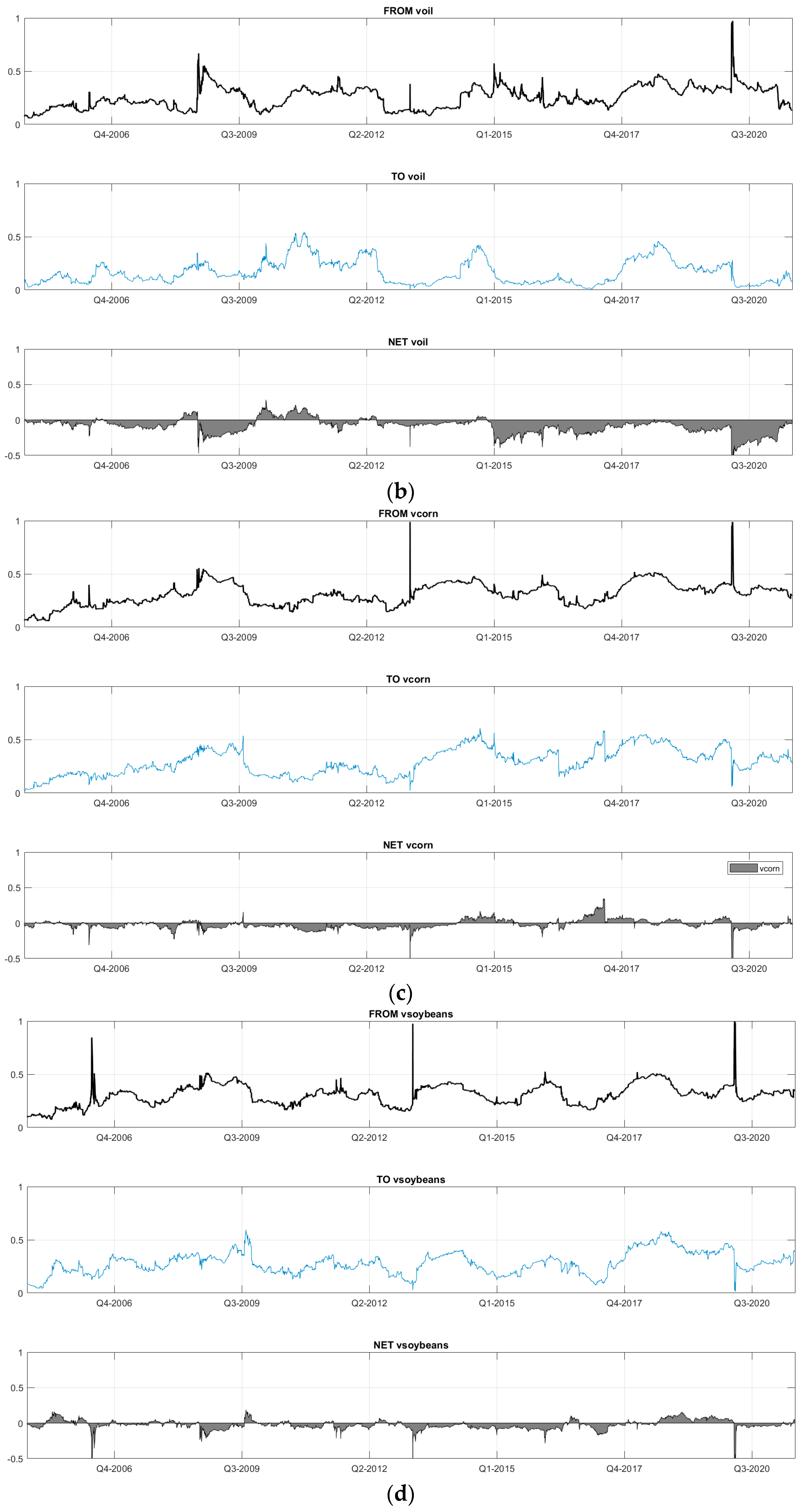
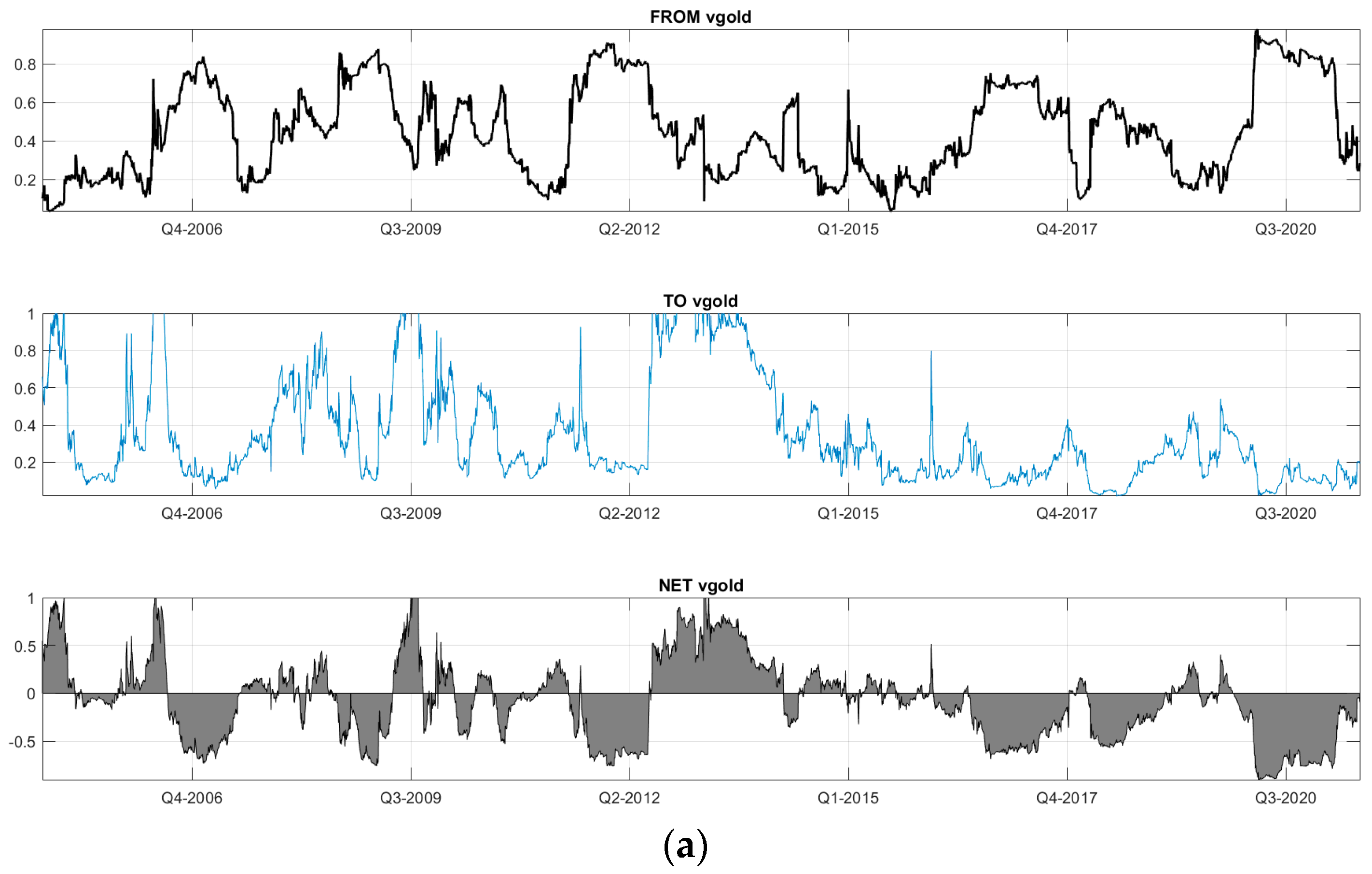
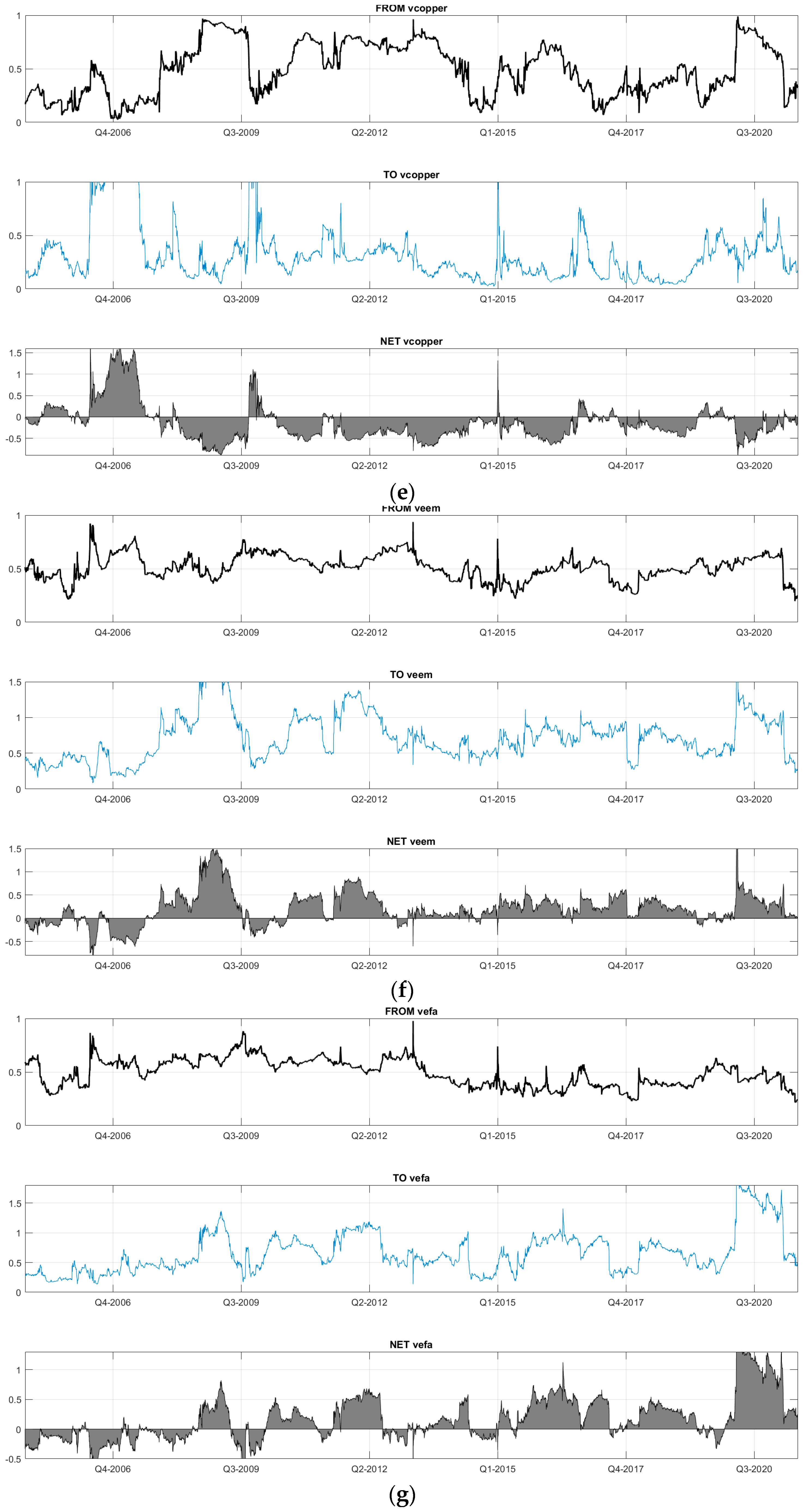
Figure 3 (a–g) displays the dynamic contribution of each variable and the system’s contribution to each variable.
A close inspection of these graphs shows that emerging equity markets are net receivers of shocks from other markets until the beginning of the subprime crisis and then turn into large-scale net contributors over the period of the subprime crisis. Except for the initial period, emerging markets show generally a net contribution to the others and this contribution is amplified in periods of major turbulence, such as the European sovereign debt crisis, the Brexit referendum, and the pandemic crisis.
For developed markets, we notice that, on the events mentioned above, developed equity markets are basically net transmitters by being net receivers during the periods that mediate these major events.
Interestingly, gold, oil, and copper which have systematically been net recipients of shocks from other markets amplified this impact very significantly during the period of the COVID surge.
The results of the variability over time in terms of directional linkage in net pairs between market volatility show how small and short the net contributions of volatility in the oil and agricultural commodities market to the volatilities of other markets are.
6. Conclusions
In this paper, we perform the analysis of the interaction of emerging markets and developed markets equity with precious metals, agricultural commodities, and one industrial commodity. Using the connectedness index based on a VAR approach, we measure how each element of a system is affected by the system’s dynamics and contributes to the system. We analyse the return and volatility spillover across the markets.
The results presented show that developed and emerging equity markets have information content for commodities markets. Our results show a significant connectedness among the returns and volatility measures around 35% over the full period analysed and that the total connectedness among market returns is higher in the short-term than in the long-term, while in the case of volatility the long-term frequencies concentrate the market connectedness.
Our results suggest that the contribution of returns and volatility shocks from emerging equity markets and developed equity markets to commodity markets is larger than the reverse.
When we analyze the temporal evolution of total connectedness and all partial directional connectedness across markets we can clearly observe that volatility and return connectedness exhibit significant variation over time, with a particular surge in periods of great instability.
The total connection of volatility is mainly driven by emerging equity market volatility shocks, as well as developed equity market volatility shocks, apart from the period before the subprime crisis, where gold and mainly copper emerge as the main net contributors to the system. The importance of this study comes not only from the fact that risk levels are critical factors in determining asset values but also from the fact that the dynamic analysis of risk and returns as well as its transmission across markets are important factors to be considered in the portfolio composition and definition of investment strategies. Once investors can make the portfolio composition considering different investment horizons, the above evidence, namely in terms of direction, intensity, and persistence of cross-shock transmissions over markets, can support them in adjusting portfolios to their risk-return preferences.
The empirical analysis conducted provides new evidence of the dynamic interactions between emerging and developed equity and commodity markets and implies that investors and fund managers in order to design appropriate hedging strategies and portfolio structures should take into account news from selected markets when there are strong spillover possibilities.
Policy makers can benefit from analysing the relationship between volatilities and returns in equity and commodity markets to assess the impact of a shock to prices in one market on the others, their levels, and scope, and thus frame regulatory policies. The analysis of drivers of the dynamics of risk transmission across markets may also be important for policy makers, as it may allow policy makers introducing mechanisms to control the transmission of risk across markets.
Author Contributions
The authors contributed equally to this work. All authors have read and agreed to the published version of the manuscript.
Funding
This research received no external funding.
Institutional Review Board Statement
Not applicable.
Informed Consent Statement
Not applicable.
Data Availability Statement
The data presented in this study is available on request from the corresponding author.
Conflicts of Interest
The authors declare no conflict of interest.
References
- Bheenick, E.; Brooks, R.; Do, H.; Smyth, R. Exploiting the heteroskedasticity in measurement error to improve volatility predictions in oil and biofuel feedstock markets. Energy Econ. 2020, 86, 104689. [Google Scholar] [CrossRef]
- Gong, X.; Lin, B. Forecasting the good and bad uncertainties of crude oil prices using HAR framework. Energy Econ. 2017, 67, 315–327. [Google Scholar] [CrossRef]
- Ma, F.; Liao, Y.; Zhang, Y.; Cao, Y. Harnessing jump component for crude oil volatility forecasting in the presence of extreme shocks. J. Empir. Financ. 2019, 52, 40–55. [Google Scholar] [CrossRef]
- Hasanov, A.; Poon, W.; Al-Freedi, A.; Heng, Z. Forecasting volatility in the biofuel feedstock mrakets in the presence of structural breaks: A comparison of alternative distribution functions. Energy Econ. 2018, 70, 307–333. [Google Scholar] [CrossRef]
- Klein, T.; Walter, T. Oil price volatility forecast with mixture memory GARCH. Energy Econ. 2016, 58, 46–58. [Google Scholar] [CrossRef] [Green Version]
- Chkili, W.; Hammoudeh, S.; Nguyen, D. Volatility forecasting and risk management for commodity markets in the presence of asymmetry and long memory. Energy Econ. 2014, 41, 1–18. [Google Scholar] [CrossRef]
- Haugom, E.; Langeland, H.; Molnar, P.; Westgaard, S. Forecasting volatility of the U.S. oil market. J. Bank. Financ. 2014, 47, 1–14. [Google Scholar] [CrossRef] [Green Version]
- Arouri, M.; Lahiani, A.; Nguyen, D.K. Forecasting the conditional volatility of oil spot and futures prices with structural breaks and long memory models. Energy Econ. 2012, 34, 283–293. [Google Scholar] [CrossRef] [Green Version]
- Sadorsky, P. Modeling volatility and correlations between emerging market stock prices and the prices of copper, oil and wheat. Energy Econ. 2014, 43, 72–81. [Google Scholar] [CrossRef]
- Filis, G. Time-varing co-movements between stock market returns and oil price shocks. Int. J. Energy Stat. 2014, 2, 27–42. [Google Scholar] [CrossRef]
- Chang, K.-L.; McAleer, M.; Tansuchat, R. Conditional correlations and volatility spillovers between crude oil and stock index returns. N. Am. J. Econ. Financ. 2013, 25, 116–138. [Google Scholar] [CrossRef] [Green Version]
- Filis, G.; Degiannakis, S.; Floros, C. Dynamic correlation between stock market and oil prices: The case of oil-importing and oil-exporting countries. Int. Rev. Financ. Anal. 2011, 20, 152–164. [Google Scholar] [CrossRef]
- Mensi, W.; Beljid, M.; Boubaker, A.; Shunsuke, M. Correlations and volatility spillovers across commodity and stock markets: Linking energies, food, and gold. Econ. Model. 2013, 32, 15–22. [Google Scholar] [CrossRef] [Green Version]
- Sarwar, S.; Tiwari, A.K.; Tingqiu, C. Analyzing volatility spillovers between oil market and Asian stock markets. Resour. Policy 2020, 66, 101608. [Google Scholar] [CrossRef]
- Khalfaoui, A.; Boutahar, M.; Boubaker, H. Analyzing volatility spillovers and hedging between oil and stock markets: Evidence from wavelet analysis. Energy Econ. 2015, 49, 540–549. [Google Scholar] [CrossRef]
- Berger, T.; Uddin, G.S. On the dynamic dependence between equity markets, commodity futures and economic uncertainty indexes. Energy Econ. 2016, 56, 374–383. [Google Scholar] [CrossRef]
- Wang, X.; Lucey, B.; Huang, S. Can gold hedge against oil price movements: Evidence from GARCH-EVT wavelet modeling. J. Commod. Mark. 2021, 100226. [Google Scholar] [CrossRef]
- Diebold, F.X.; Yilmaz, K. Measuring financial asset return and volatility spillovers, with application to global equity markets. Econ. J. 2009, 119, 158–171. [Google Scholar] [CrossRef] [Green Version]
- Diebold, F.X.; Yilmaz, K. Better to Give than to Receive: Forecast-Based Measurement of Volatility Spillovers. Int. J. Forecast. 2012, 28, 57–66. [Google Scholar] [CrossRef] [Green Version]
- Kumar, M. Returns and volatility spillover between stock prices and exchange rates: Empirical evidence from IBSA countries. Int. J. Emerg. Mark. 2013, 8, 108–128. [Google Scholar] [CrossRef]
- Maghyereh, A.I.; Awartani, B.; Bouri, E. The directional volatility connectedness between crude oil and equity markets: New evidence from implied volatility indexes. Energy Econ. 2016, 57, 78–93. [Google Scholar] [CrossRef] [Green Version]
- Caloia, F.G.; Cipollini, A.; Muzzioli, S. Asymmetric semi-volatility spillover effects in EMU stock markets. Int. Rev. Financ. Anal. 2018, 57, 221–230. [Google Scholar] [CrossRef]
- Mensi, W.; Hkiri, B.; Al-Yahyaee, K.; Kang, S.H. Analyzing time–frequency co-movements across gold and oil prices with BRICS stock markets: A VaR based on wavelet approach. Int. Rev. Econ. Finance 2018, 54, 74–102. [Google Scholar] [CrossRef]
- BenSaïda, A.; Litimi, H.; Abdallah, O. Volatility spillover shifts in global financial markets. Econ. Model. 2018, 73, 343–353. [Google Scholar] [CrossRef]
- Yoon, S.-M.; Al Mamun, M.; Uddin, G.S.; Kang, S.H. Network connectedness and net spillover between financial and commodity markets. N. Am. J. Econ. Financ. 2019, 48, 801–818. [Google Scholar] [CrossRef]
- Balcilar, M.; Ozdemir, Z.A.; Ozdemir, H. Dynamic return and volatility spillovers among S&P 500, crude oil, and gold. Int. J. Financ. Econ. 2021, 26, 153–170. [Google Scholar]
- Akhtaruzzaman, M.; Boubaker, S.; Lucey, B.M.; Sensoy, A. Is gold a hedge or a safe-haven asset in the COVID–19 crisis? Econ. Model. 2021, 102, 105588. [Google Scholar] [CrossRef]
- Kang, S.; Hernandez, J.A.; Sadorsky, P.; McIver, R. Frequency spillovers, connectedness, and the hedging effectiveness of oil and gold for US sector ETFs. Energy Econ. 2021, 99, 105278. [Google Scholar] [CrossRef]
- Barunik, J.; Krehlik, T. Measuring the frequency dynamics of financial connectedness and systemic risk. J. Financ. Econ. 2018, 16, 271–296. [Google Scholar] [CrossRef]
Figure 1.
The figure presents the pairwise net directional connectedness. Figure presents the pairwise net directional connectedness (left: price volatility; right: price returns). Note: The red color signifies the highest net transmitter, whereas blue lines signify the highest net recipient.
Figure 1.
The figure presents the pairwise net directional connectedness. Figure presents the pairwise net directional connectedness (left: price volatility; right: price returns). Note: The red color signifies the highest net transmitter, whereas blue lines signify the highest net recipient.
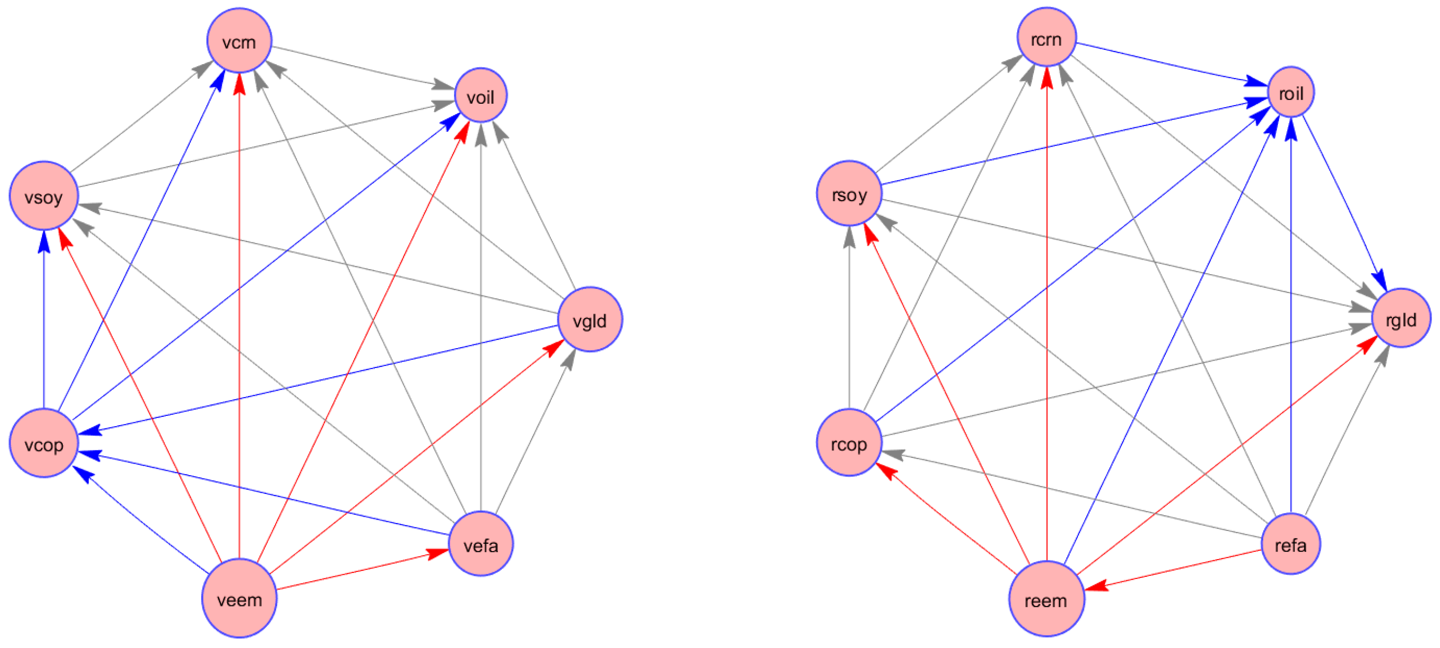
Figure 2.
Total spillover: Spillovers from volatility over the sampling period spanning from January 2005 to June 2021. Notes: (a) Bernanke: Energy and the economy speech; (b) US Subprime crisis: Collapse of two Bear Stearns hedge funds; (c) Bankruptcy of Lehman Brothers; (d) Greece bailout; (e) End of ECB Securities Market Programme; (f) Announcement by Draghi that ECB would do “whatever it takes to save the Euro”; (g) European stock market collapse; (h) Brexit referendum; (i) COVID-19 pandemic.
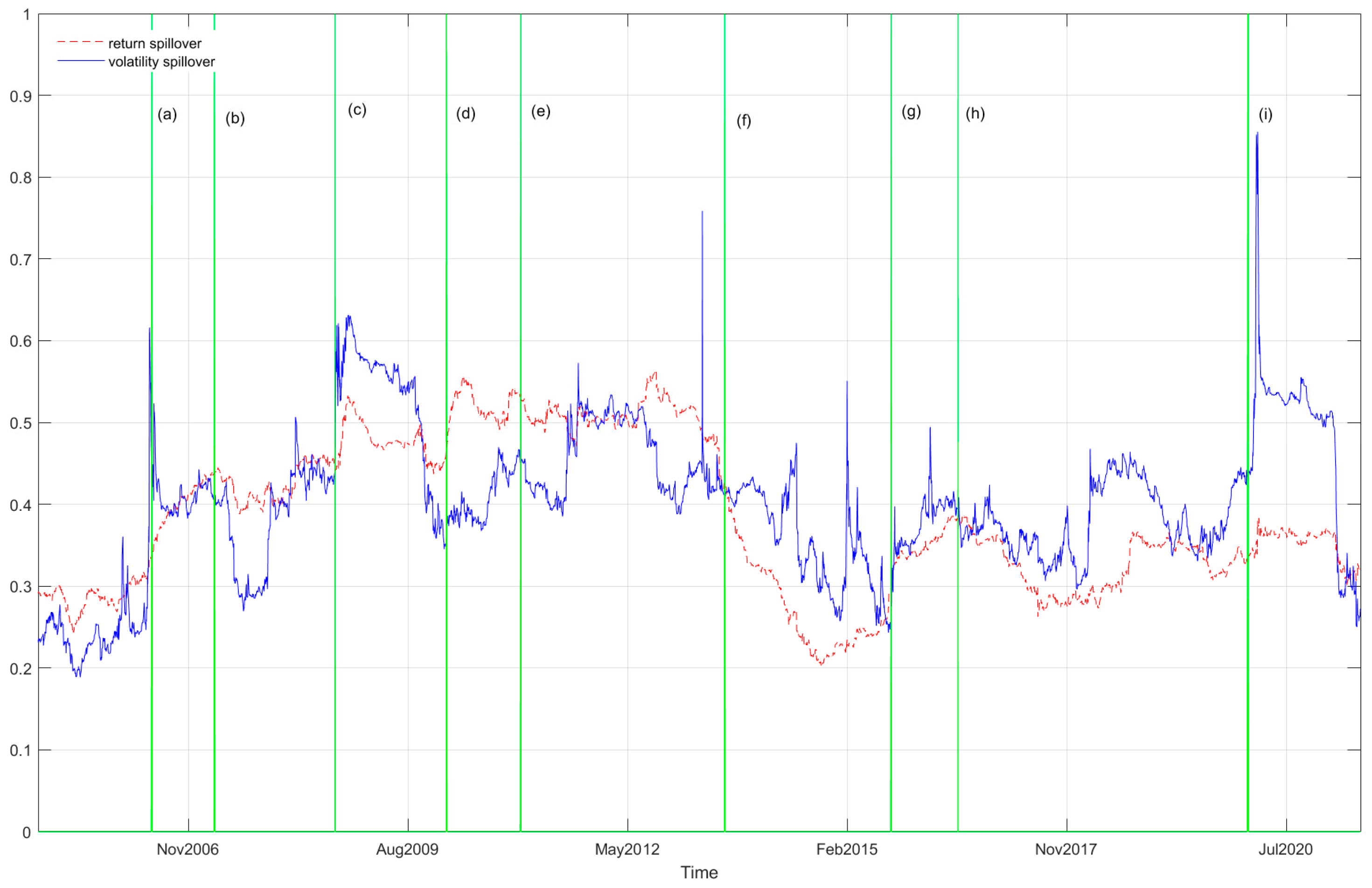
Figure 3.
(a) Rolling-windows of Gold, From/To/Net Volatility Spillovers. (b) Rolling-windows of Oil, From/To/Net Spillovers. (c) Rolling-windows of Corn, From/To/Net Spillovers. (d) Rolling-windows of Soybeans, From/To/Net Spillovers. (e) Rolling-windows of Copper, From/To/Net Spillovers. (f) Rolling-windows of EEM, From/To/Net Spillovers. (g) Rolling-windows of EFA, From/To/Net Spillovers.


Table 1.
Descriptive statistics for returns and natural logarithm volatility series.
| Variables | Mean | Std. Dev. | Min | Max | Skew. | Kurt. | JB | ADF |
|---|---|---|---|---|---|---|---|---|
| Panel A: Returns | ||||||||
| Gold | 0.033 | 1.149 | −9.821 | 8.643 | −0.344 | 8.424 | 0.0000 | −61.379 ** |
| Oil | 0.057 | 2.279 | −27.992 | 31.963 | 1.075 | 28.583 | 0.0000 | −53.306 ** |
| Soybeans | 0.02 | 1.4 | −13.843 | 20.321 | −0.036 | 20.031 | 0.0000 | −47.913 ** |
| Corn | 0.015 | 1.587 | −10.409 | 12.757 | 0.001 | 7.495 | 0.0000 | −50.865 ** |
| Copper | 0.033 | 1.799 | −11.693 | 11.769 | −0.202 | 7.168 | 0.0000 | −65.749 ** |
| EEM | 0.026 | 1.84 | −17.633 | 20.514 | 0.015 | 18.067 | 0.0000 | −73.936 ** |
| EFA | 0.013 | 1.387 | −11.837 | 14.745 | −0.407 | 16.566 | 0.0000 | −73.898 ** |
| Panel B: Volatility | ||||||||
| Gold | 2.809 | 0.263 | 2.35 | 3.73 | 0.962 | 3.676 | 0.0000 | −3.757 ** |
| Oil | 3.636 | 0.202 | 3.146 | 5.65 | 2.088 | 18.276 | 0.0000 | −4.464 ** |
| Soybeans | 3.174 | 0.154 | 2.858 | 4.741 | 2.251 | 14.042 | 0.0000 | −3.092 * |
| Corn | 3.319 | 0.129 | 3.043 | 4.474 | 2.382 | 14.614 | 0.0000 | −3.546 ** |
| Copper | 3.221 | 0.304 | 2.668 | 4.424 | 0.988 | 4.281 | 0.0000 | −3.618 ** |
| EEM | 3.103 | 0.387 | 2.468 | 5.008 | 1.562 | 6.651 | 0.0000 | −4.215 ** |
| EFA | 2.817 | 0.42 | 2.055 | 4.701 | 1.267 | 5.358 | 0.0000 | −4.584 ** |
Notes: This table presents the main descriptive statistics of the returns and volatility of prices and indices, as well as the results of the respective normality tests. Panel A shows returns; Panel B shows log-transformed volatility series. ** and * denote significance at 1% and 5%, respectively.
Table 2.
Correlation matrix.
| Panel A: Returns | |||||||
| Variables | (1) | (2) | (3) | (4) | (5) | (6) | (7) |
| (1) Gold | 1.000 | ||||||
| (2) Oil | 0.182 * | 1.000 | |||||
| (3) Soybeans | 0.146 * | 0.217 * | 1.000 | ||||
| (4) Corn | 0.147 * | 0.213 * | 0.563 * | 1.000 | |||
| (5) Copper | 0.339 * | 0.294 * | 0.222 * | 0.191 * | 1.000 | ||
| (6) EEM | 0.123 * | 0.252 * | 0.153 * | 0.130 * | 0.367 * | 1.000 | |
| (7) EFA | 0.120 * | 0.251 * | 0.143 * | 0.133 * | 0.370 * | 0.879 * | 1.000 |
| Panel B: Volatility | |||||||
| Variables | (1) | (2) | (3) | (4) | (5) | (6) | (7) |
| (1) Gold | 1.000 | ||||||
| (2) Oil | 0.232 * | 1.000 | |||||
| (3) Soybeans | 0.133 * | 0.067 * | 1.000 | ||||
| (4) Corn | 0.145 * | 0.108 * | 0.447 * | 1.000 | |||
| (5) Copper | 0.693 * | 0.180 * | 0.157 * | 0.173 * | 1.000 | ||
| (6) EEM | 0.721 * | 0.292 * | 0.153 * | 0.160 * | 0.722 * | 1.000 | |
| (7) EFA | 0.682* | 0.308 * | 0.135 * | 0.165 * | 0.639 * | 0.931 * | 1.000 |
* p < 0.1.
Table 3.
Volatility and return spillover table.
| Volatility Spillover Table Rows (to), Columns (from), | |||||||||
| Gold | Oil | Soybeans | Corn | Copper | eem | efa | From Others | NDC | |
| gold | 51.497 | 0.518 | 0.307 | 0.316 | 2.057 | 23.817 | 21.487 | 48.503 | −25.709 |
| oil | 0.885 | 82.208 | 1.629 | 1.745 | 1.280 | 6.445 | 5.809 | 17.792 | −12.259 |
| soybeans | 0.635 | 1.397 | 76.634 | 17.360 | 1.324 | 1.148 | 1.502 | 23.366 | −3.487 |
| corn | 0.712 | 1.497 | 16.999 | 77.991 | 1.193 | 0.914 | 0.694 | 22.009 | −1.000 |
| copper | 9.936 | 0.672 | 0.413 | 1.003 | 47.631 | 24.688 | 15.658 | 52.369 | −38.516 |
| eem | 5.791 | 0.635 | 0.292 | 0.364 | 4.725 | 52.963 | 35.230 | 47.037 | 47.184 |
| efa | 4.834 | 0.815 | 0.239 | 0.222 | 3.274 | 37.210 | 53.408 | 46.592 | 33.787 |
| Contribution to others | 22.793 | 5.534 | 19.879 | 21.009 | 13.852 | 94.222 | 80.379 | ||
| Returns Spillover Table Rows (to), Columns (from), | |||||||||
| Gold | Oil | Soybeans | Corn | Copper | eem | efa | From Others | NDC | |
| gold | 81.240 | 2.770 | 1.800 | 1.730 | 8.970 | 1.950 | 1.540 | 18.760 | −4.110 |
| oil | 2.630 | 74.430 | 3.400 | 3.550 | 6.480 | 4.810 | 4.690 | 25.560 | −4.720 |
| soybeans | 1.460 | 3.170 | 68.450 | 21.680 | 2.430 | 1.400 | 1.410 | 31.550 | −1.060 |
| corn | 1.510 | 3.320 | 21.230 | 67.060 | 3.310 | 1.880 | 1.700 | 32.950 | −0.440 |
| copper | 6.930 | 5.340 | 2.190 | 3.000 | 63.170 | 9.900 | 9.470 | 36.830 | −1.340 |
| eem | 1.090 | 3.180 | 0.930 | 1.330 | 7.190 | 48.510 | 37.760 | 51.480 | 6.000 |
| efa | 1.030 | 3.060 | 0.940 | 1.220 | 7.110 | 37.540 | 49.090 | 50.900 | 5.670 |
| Contribution to others | 14.650 | 20.840 | 30.490 | 32.510 | 35.490 | 57.480 | 56.570 | ||
Notes: From others—directional spillover indices measure spillovers from all indexes j to index i; Contribution to others—directional spillover indices measure spillovers from index i to all indexes j; NDC refers to net directional connectedness, which reports the difference between To and From for each variable. Other columns contain net pairwise (i,j)-th spillovers volatility and returns of gold, oil, soybeans, corn, copper, eem and efa represent gold, oil, soybeans, corn, copper, emerging stock markets and developed markets, respectively.
Table 4.
Return spillover table for selected frequencies.
| Panel A: Spillovers Freq. Short-Term. Band 3.14 to 0.63, Corresponding to 1 Days to 5 Days. | |||||||||
| Gold | Oil | Soybeans | Corn | Copper | eem | efa | FROM_ABS | FROM_WTH | |
| gold | 66.200 | 2.180 | 1.390 | 1.430 | 7.610 | 1.270 | 1.100 | 2.14 | 2.59 |
| oil | 2.140 | 59.600 | 2.930 | 2.830 | 5.490 | 3.850 | 3.790 | 3 | 3.64 |
| soybeans | 1.390 | 2.970 | 53.600 | 17.360 | 2.840 | 1.460 | 1.270 | 3.9 | 4.72 |
| corn | 1.210 | 2.730 | 17.840 | 55.870 | 2.120 | 1.130 | 1.100 | 3.73 | 4.52 |
| copper | 5.620 | 4.380 | 2.380 | 1.740 | 53.110 | 7.520 | 7.430 | 4.15 | 5.03 |
| eem | 0.770 | 2.780 | 1.150 | 0.780 | 6.050 | 41.820 | 32.900 | 6.35 | 7.69 |
| efa | 0.710 | 2.590 | 1.060 | 0.760 | 5.890 | 31.750 | 41.850 | 6.11 | 7.4 |
| TO_ABS | 1.69 | 2.52 | 3.82 | 3.56 | 4.29 | 6.71 | 6.8 | 29.39 | |
| TO_WTH | 2.05 | 3.05 | 4.63 | 4.31 | 5.19 | 8.13 | 8.24 | 35.6 | |
| NET ABS | −0.45 | −0.48 | −0.08 | −0.17 | 0.14 | 0.36 | 0.69 | ||
| Panel B: Spillovers Freq. Medium-Term. Band 0.63 to 0.15, Corresponding to 5 Days to 21 Days. | |||||||||
| Gold | Oil | Soybeans | Corn | Copper | eem | efa | FROM_ABS | FROM_WTH | |
| gold | 11.100 | 0.440 | 0.250 | 0.270 | 1.010 | 0.500 | 0.320 | 0.4 | 3.1 |
| oil | 0.350 | 10.870 | 0.460 | 0.420 | 0.730 | 0.700 | 0.660 | 0.47 | 3.68 |
| soybeans | 0.100 | 0.270 | 9.880 | 2.850 | 0.340 | 0.310 | 0.310 | 0.6 | 4.63 |
| corn | 0.180 | 0.330 | 2.840 | 9.290 | 0.230 | 0.200 | 0.230 | 0.57 | 4.46 |
| copper | 0.960 | 0.710 | 0.450 | 0.330 | 7.450 | 1.750 | 1.510 | 0.82 | 6.33 |
| eem | 0.230 | 0.300 | 0.130 | 0.110 | 0.850 | 4.970 | 3.620 | 0.75 | 5.81 |
| efa | 0.230 | 0.350 | 0.110 | 0.130 | 0.900 | 4.280 | 5.350 | 0.86 | 6.67 |
| TO_ABS | 0.29 | 0.34 | 0.61 | 0.59 | 0.58 | 1.11 | 0.95 | 4.47 | |
| TO_WTH | 2.28 | 2.65 | 4.7 | 4.57 | 4.52 | 8.6 | 7.37 | 34.68 | |
| NET ABS | −0.11 | −0.13 | 0.01 | 0.02 | −0.24 | 0.36 | 0.09 | ||
| Pabel C: Spillovers Freq. Long-Term. Band 0.15 to 0.01, Corresponding to More than 21 Days. | |||||||||
| Long_Term | Gold | Oil | Soybeans | Corn | Copper | eem | efa | FROM_ABS | FROM_WTH |
| gold | 3.950 | 0.150 | 0.090 | 0.090 | 0.350 | 0.180 | 0.110 | 0.11 | 3.05 |
| oil | 0.140 | 3.960 | 0.160 | 0.150 | 0.260 | 0.260 | 0.240 | 0.14 | 3.78 |
| soybeans | 0.030 | 0.080 | 3.580 | 1.020 | 0.130 | 0.110 | 0.110 | 0.17 | 4.6 |
| corn | 0.060 | 0.110 | 1.000 | 3.290 | 0.080 | 0.070 | 0.080 | 0.16 | 4.38 |
| copper | 0.350 | 0.250 | 0.160 | 0.120 | 2.620 | 0.620 | 0.530 | 0.23 | 6.37 |
| eem | 0.090 | 0.100 | 0.040 | 0.040 | 0.300 | 1.720 | 1.250 | 0.21 | 5.69 |
| efa | 0.090 | 0.120 | 0.040 | 0.050 | 0.320 | 1.510 | 1.880 | 0.24 | 6.63 |
| TO_ABS | 0.29 | 0.34 | 0.61 | 0.59 | 0.58 | 1.11 | 0.95 | 1.26 | |
| TO_WTH | 0.09 | 0.09 | 0.17 | 0.17 | 0.16 | 0.31 | 0.27 | 34.49 | |
| NET ABS | −0.02 | −0.05 | 0 | 0.01 | −0.07 | 0.1 | 0.03 | ||
Notes: “FROM_ABS” correspond to “Absolute to” is the measure of “frequency” connectedness from market j to other markets, and “FROM_WTH” is the measure of “within” connectedness; “NET ABS” refers to net directional connectedness, which reports the difference between TO ABS and FROM ABS for each variable. Other columns contain net pairwise (i,j)-th spillovers returns at the frequency band of gold, oil, soybeans, corn, copper, eem and efa represent gold, oil, soybeans, corn, copper, emerging stock markets and developed markets, respectively.
Table 5.
Volatility spillover table for selected frequencies.
| Panel A: Spillovers Freq. Short-Term. Band 3.14 to 0.63, Corresponding to 1 Days to 5 Days. | |||||||||
| Gold | Oil | Soybeans | Corn | Copper | eem | efa | FROM_ABS | FROM_WTH | |
| gold | 0.370 | 0.000 | 0.000 | 0.000 | 0.000 | 0.030 | 0.030 | 0.01 | 0.03 |
| oil | 0.100 | 56.710 | 1.490 | 1.360 | 0.540 | 0.130 | 0.170 | 0.54 | 2.08 |
| soybeans | 0.100 | 1.290 | 48.500 | 10.860 | 0.210 | 0.110 | 0.050 | 1.8 | 6.93 |
| corn | 0.030 | 1.090 | 10.290 | 45.870 | 0.110 | 0.120 | 0.080 | 1.67 | 6.44 |
| copper | 0.010 | 0.000 | 0.000 | 0.000 | 0.380 | 0.050 | 0.040 | 0.01 | 0.06 |
| eem | 0.000 | 0.000 | 0.000 | 0.000 | 0.000 | 0.590 | 0.260 | 0.04 | 0.15 |
| efa | 0.000 | 0.000 | 0.000 | 0.000 | 0.000 | 0.340 | 0.800 | 0.05 | 0.19 |
| TO_ABS | 0.04 | 0.34 | 1.68 | 1.75 | 0.12 | 0.11 | 0.09 | 4.13 | |
| TO_WTH | 0.14 | 1.31 | 6.47 | 6.71 | 0.48 | 0.42 | 0.35 | 15.87 | |
| NET ABS | 0.03 | −0.2 | −0.12 | 0.08 | 0.11 | 0.07 | 0.04 | ||
| Panel B: Spillovers Freq. Medium-Term. Band 0.63 to 0.15, Corresponding to 5 Days to 21 Days. | |||||||||
| Gold | Oil | Soybeans | Corn | Copper | eem | efa | FROM_ABS | FROM_WTH | |
| gold | 1.040 | 0.000 | 0.000 | 0.000 | 0.020 | 0.040 | 0.060 | 0.02 | 0.16 |
| oil | 0.030 | 18.400 | 0.180 | 0.180 | 0.230 | 0.200 | 0.210 | 0.15 | 1.28 |
| soybeans | 0.060 | 0.150 | 21.140 | 4.420 | 0.110 | 0.070 | 0.030 | 0.69 | 5.97 |
| corn | 0.020 | 0.190 | 5.010 | 22.120 | 0.080 | 0.090 | 0.070 | 0.78 | 6.72 |
| copper | 0.030 | 0.000 | 0.010 | 0.000 | 1.150 | 0.130 | 0.130 | 0.04 | 0.37 |
| eem | 0.010 | 0.010 | 0.010 | 0.000 | 0.020 | 1.610 | 0.700 | 0.11 | 0.93 |
| efa | 0.020 | 0.020 | 0.000 | 0.000 | 0.010 | 0.910 | 2.190 | 0.14 | 1.19 |
| TO_ABS | 0.03 | 0.05 | 0.74 | 0.66 | 0.07 | 0.21 | 0.17 | 1.93 | |
| TO_WTH | 0.22 | 0.47 | 6.42 | 5.68 | 0.57 | 1.77 | 1.49 | 16.61 | |
| NET ABS | 0.01 | −0.1 | 0.05 | −0.12 | 0.03 | 0.1 | 0.03 | ||
| Panel C: Spillovers Freq. Long-Term. Band 0.15 to 0.01, Corresponding to More than 21 Days. | |||||||||
| Long_Term | Gold | Oil | Soybeans | Corn | Copper | eem | efa | FROM_ABS | FROM_WTH |
| gold | 50.040 | 0.520 | 0.310 | 0.300 | 2.050 | 23.790 | 21.390 | 6.91 | 11.07 |
| oil | 0.750 | 7.090 | 0.070 | 0.090 | 0.520 | 6.120 | 5.420 | 1.85 | 2.97 |
| soybeans | 0.550 | 0.050 | 8.340 | 1.720 | 0.890 | 0.740 | 0.610 | 0.65 | 1.04 |
| corn | 0.570 | 0.110 | 2.060 | 8.640 | 1.140 | 0.950 | 1.360 | 0.88 | 1.42 |
| copper | 9.860 | 0.670 | 0.990 | 0.410 | 46.130 | 24.530 | 15.470 | 7.42 | 11.89 |
| eem | 5.760 | 0.620 | 0.360 | 0.290 | 4.720 | 50.780 | 34.250 | 6.57 | 10.53 |
| efa | 4.800 | 0.790 | 0.220 | 0.230 | 3.280 | 35.980 | 50.400 | 6.47 | 10.37 |
| TO_ABS | 3.19 | 0.39 | 0.57 | 0.43 | 1.8 | 13.16 | 11.21 | 30.76 | |
| TO_WTH | 5.11 | 0.63 | 0.92 | 0.7 | 2.88 | 21.09 | 17.98 | 49.3 | |
| NET ABS | −3.72 | −1.46 | −0.08 | −0.45 | −5.62 | 6.59 | 4.74 | ||
Notes: “FROM_ABS” correspond to “Absolute to” is the measure of “frequency” connectedness from market j to other markets, and “FROM_WTH” is the measure of “within” connectedness; “NET ABS” refers to net directional connectedness, which reports the difference between TO ABS and FROM ABS for each variable/market. Other columns contain net pairwise (i,j)-th spillovers volatility at the frequency band of gold, oil, soybeans, corn, copper, eem and efa represent gold, oil, soybeans, corn, copper, emerging stock markets and developed markets, respectively.
Publisher’s Note: MDPI stays neutral with regard to jurisdictional claims in published maps and institutional affiliations. |
© 2022 by the authors. Licensee MDPI, Basel, Switzerland. This article is an open access article distributed under the terms and conditions of the Creative Commons Attribution (CC BY) license (https://creativecommons.org/licenses/by/4.0/).
Share and Cite
MDPI and ACS Style
Pinho, C.; Maldonado, I. Commodity and Equity Markets: Volatility and Return Spillovers. Commodities 2022, 1, 18-33. https://doi.org/10.3390/commodities1010003
AMA Style
Pinho C, Maldonado I. Commodity and Equity Markets: Volatility and Return Spillovers. Commodities. 2022; 1(1):18-33. https://doi.org/10.3390/commodities1010003
Chicago/Turabian StylePinho, Carlos, and Isabel Maldonado. 2022. "Commodity and Equity Markets: Volatility and Return Spillovers" Commodities 1, no. 1: 18-33. https://doi.org/10.3390/commodities1010003