
Identification and Predictive Value of Risk Factors for Mortality Due to Listeria monocytogenes Infection: Use of Machine Learning with a Nationwide Administrative Data Set

 ,
,
Abstract
:1. Introduction
1.1. Listeriosis
1.2. Statistical Approaches to Predicting Outcomes from Electronic Health Records (EHR)
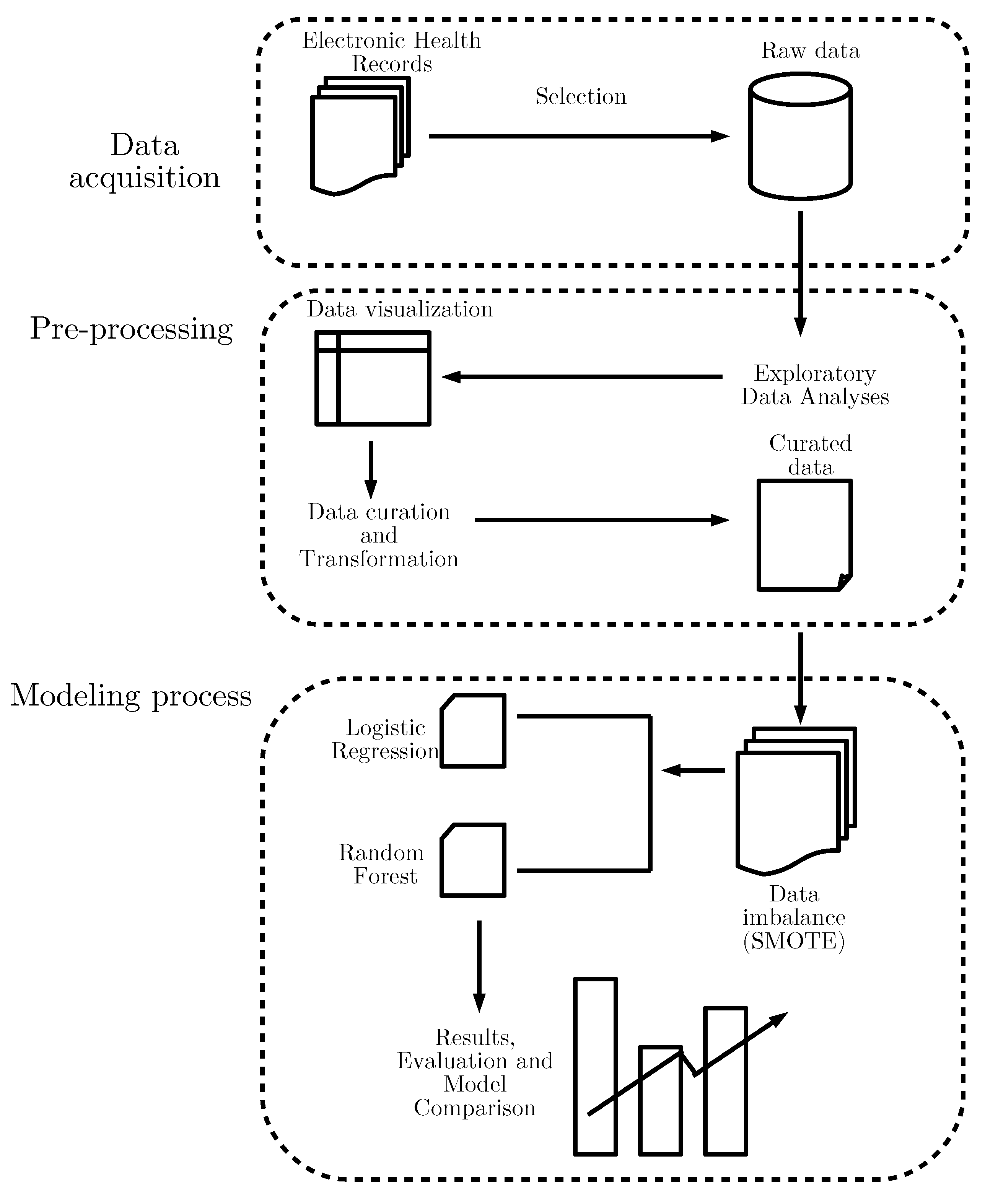
2. Materials and Methods
2.1. Data Collection
2.2. Feature Engineering and the Building of the Data Set
2.3. Definitions of Variables: ICD-9 Codes
2.4. Definitions of Variables: ICD-10-CM Codes
2.5. Statistical Analyses
2.5.1. Descriptive Analyses and Bivariate Analyses
2.5.2. Multivariate Analysis Using LR
2.5.3. Feature Selection Using RF
2.5.4. Data Splitting and Performance Metrics
3. Results
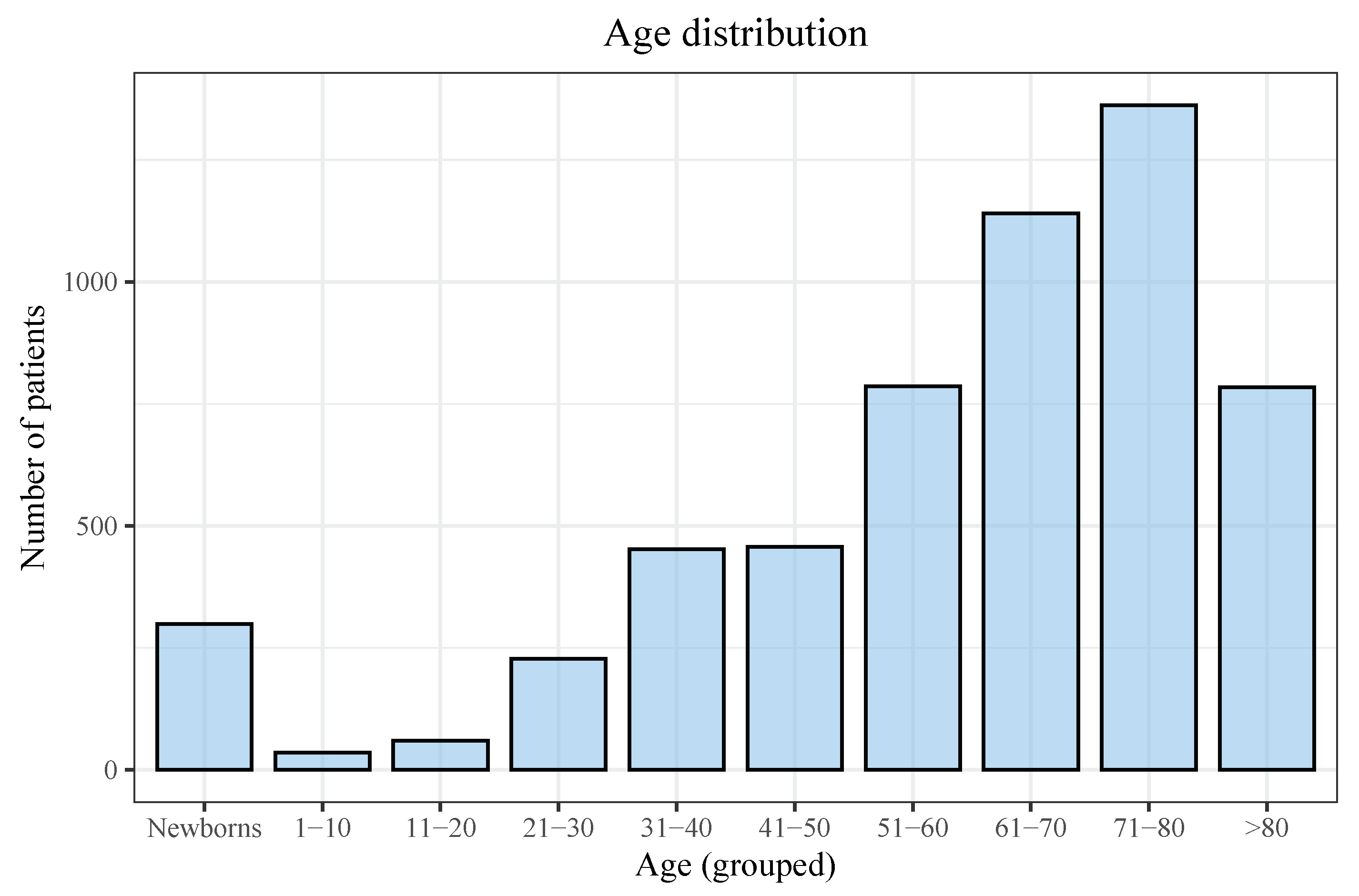
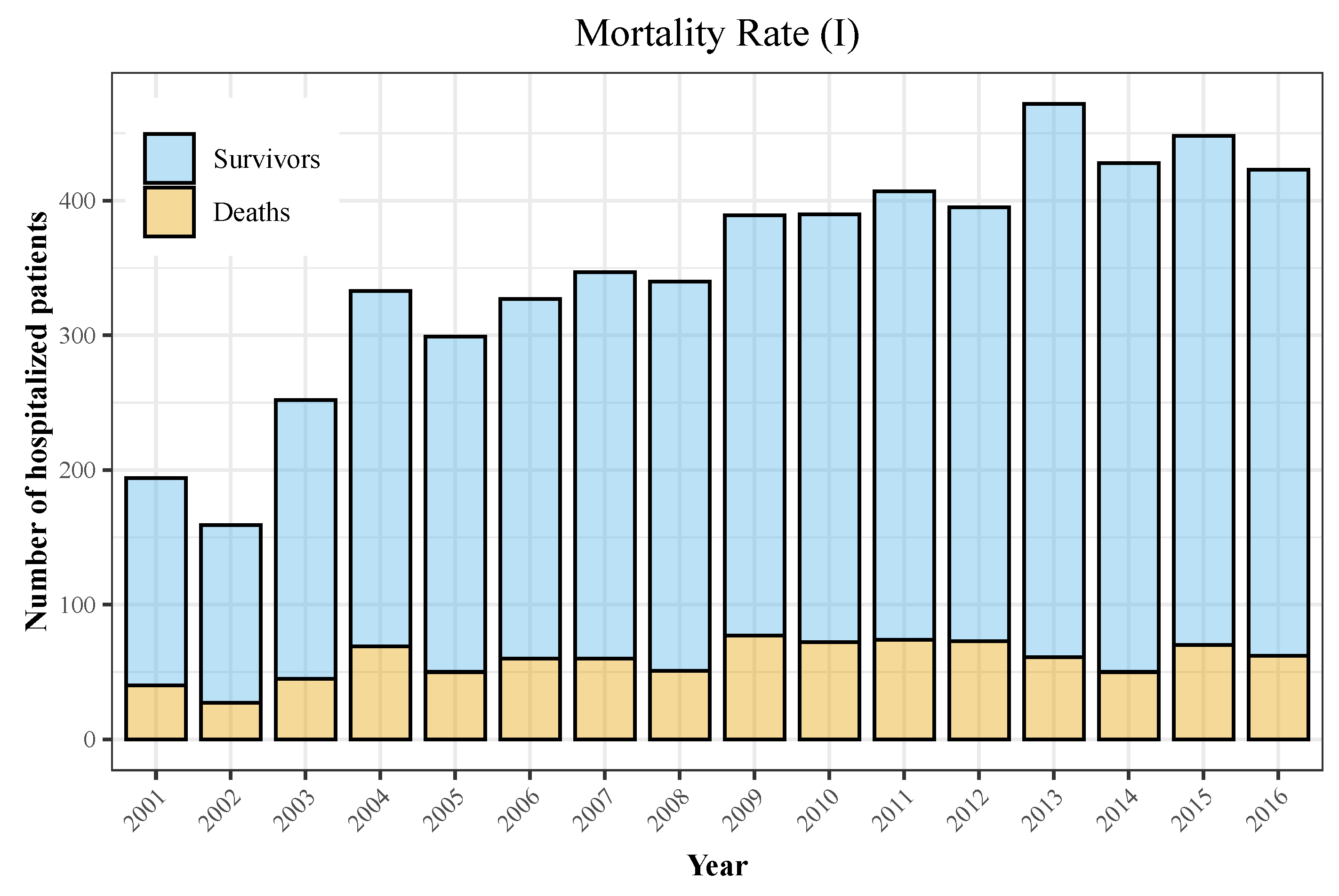
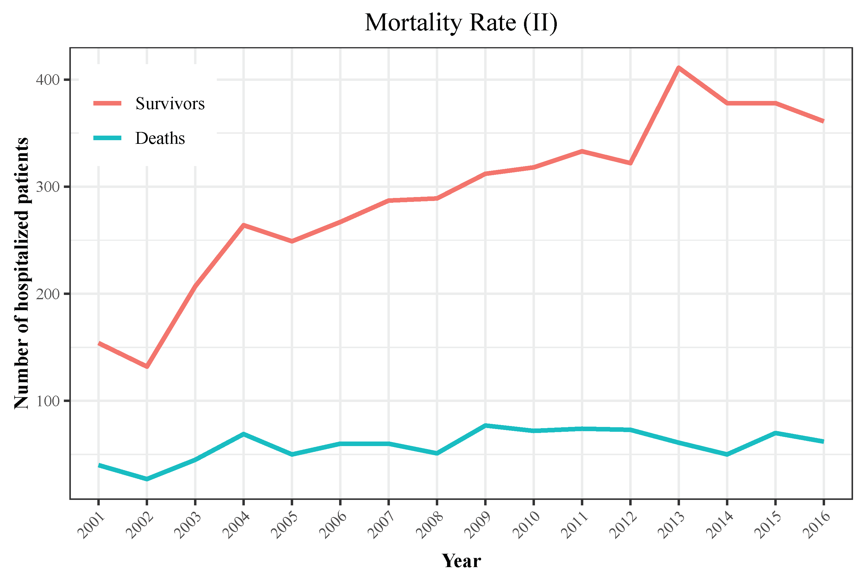
3.1. Descriptive Analyses
3.2. Bivariate Analyses and LR
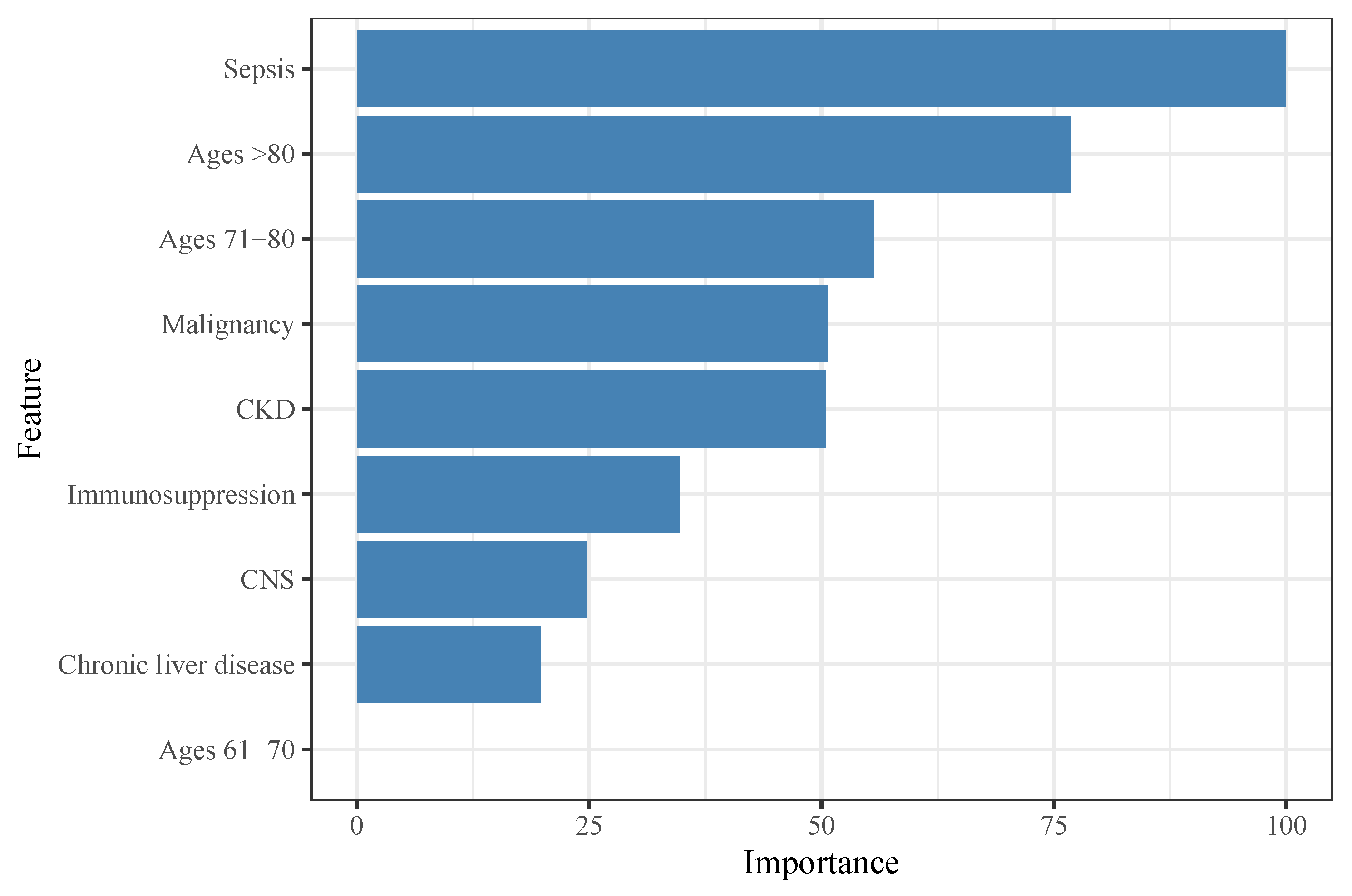
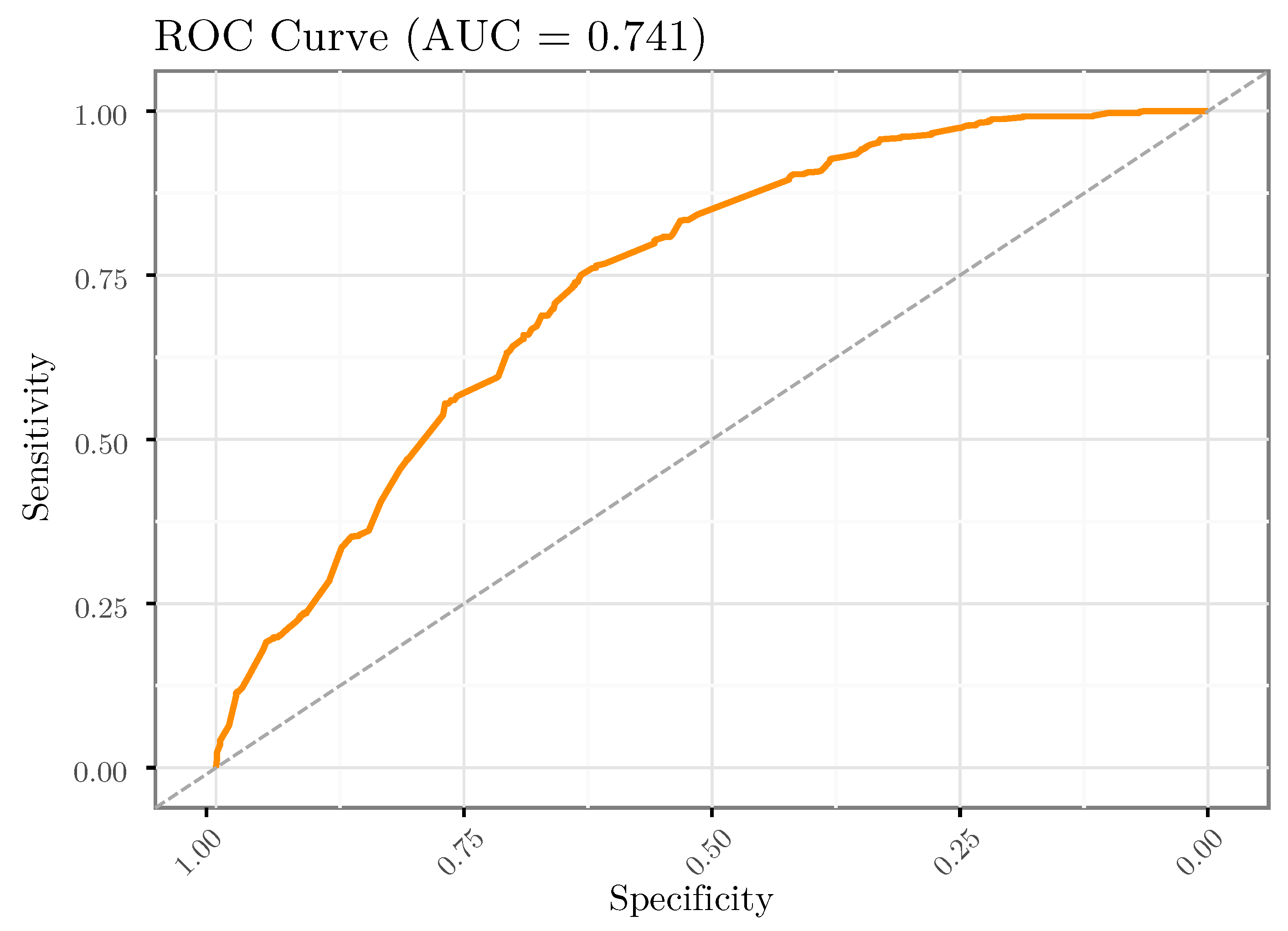
3.3. RF-Based Analyses and Interpretation
4. Discussion
4.1. Descriptive Analyses
4.2. Statistics and Machine Learning
4.3. Relevant Features of Listeria-Related Mortality
4.4. Limitations: The Reliability of Administrative Data
5. Conclusions
Author Contributions
Funding
Institutional Review Board Statement
Informed Consent Statement
Data Availability Statement
Conflicts of Interest
Abbreviations
| CKD | chronic kidney disease |
| CNS | central nervous system |
| CSF | cerebrospinal fluid |
| EHR | electronic health records |
| ICD-9 | International Classification of Diseases, Ninth Revision |
| ICD-10-CM | International Classification of Diseases, Tenth Revision, Clinical Modification |
| IQR | interquartile range |
| LIME | Local Interpretable Model-Agnostic Explanations |
| LR | logistic regression |
| MBDS-H | Spanish Minimum Basic Data Set at Hospitalization |
| OR | odds ratio |
| RF | random forest |
| SMOTE | synthetic minority over-sampling technique |
References
- Farber, J.M.; Peterkin, P.I. Listeria monocytogenes, a food-borne pathogen. Microbiol. Rev. 1991, 55, 476–511. [Google Scholar] [CrossRef]
- Swaminathan, B.; Gerner-Smidt, P. The epidemiology of human listeriosis. Microbes Infect. 2007, 9, 1236–1243. [Google Scholar] [CrossRef] [Green Version]
- Lorber, B. Listeria Monocytogenes. In Mandell, Douglas, and Bennett’s Principles and Practice of Infectious Diseases, 8th ed.; Bennett, J., Dolin, R., Blaser, M., Eds.; Elsevier/Saunders: Philadelphia, PA, USA, 2015; pp. 2383–2390.e2. [Google Scholar] [CrossRef]
- Elinav, H.; Hershko-Klement, A.; Valinsky, L.; Jaffe, J.; Wiseman, A.; Shimon, H.; Braun, E.; Paitan, Y.; Block, C.; Sorek, R.; et al. Pregnancy-associated listeriosis: Clinical characteristics and geospatial analysis of a 10-year period in Israel. Clin. Infect. Dis. 2014, 59, 953–961. [Google Scholar] [CrossRef] [Green Version]
- Wadhwa Desai, R.; Smith, M.A. Pregnancy-related listeriosis. Birth Defects Res. 2017, 109, 324–335. [Google Scholar] [CrossRef] [PubMed] [Green Version]
- Arslan, F.; Meynet, E.; Sunbul, M.; Sipahi, O.R.; Kurtaran, B.; Kaya, S.; Inkaya, A.C.; Pagliano, P.; Sengoz, G.; Batirel, A.; et al. The clinical features, diagnosis, treatment, and prognosis of neuroinvasive listeriosis: A multinational study. Eur. J. Clin. Microbiol. Infect. Dis. 2015, 34, 1213–1221. [Google Scholar] [CrossRef] [PubMed]
- Pagliano, P.; Ascione, T.; Boccia, G.; De Caro, F.; Esposito, S. Listeria monocytogenes meningitis in the elderly: Epidemiological, clinical and therapeutic findings. Le Infez. Med. 2016, 24, 105–111. [Google Scholar]
- Rajkomar, A.; Oren, E.; Chen, K.; Dai, A.M.; Hajaj, N.; Hardt, M.; Liu, P.J.; Liu, X.; Marcus, J.; Sun, M.; et al. Scalable and accurate deep learning with electronic health records. NPJ Digit. Med. 2018, 1, 18. [Google Scholar] [CrossRef] [PubMed]
- Eyduran, E. Usage of penalized maximum likelihood estimation method in medical research: An alternative to maximum likelihood estimation method. J. Res. Med. Sci. 2008, 13, 325–330. [Google Scholar]
- Rajkomar, A.; Dean, J.; Kohane, I. Machine Learning in Medicine. N. Engl. J. Med. 2019, 380, 1347–1358. [Google Scholar] [CrossRef]
- Beam, A.L.; Kohane, I.S. Big data and machine learning in health care. JAMA 2018, 319, 1317–1318. [Google Scholar] [CrossRef]
- Obermeyer, Z.; Emanuel, E.J. Predicting the Future—Big Data, Machine Learning, and Clinical Medicine. N. Engl. J. Med. 2016, 375, 1216–1219. [Google Scholar] [CrossRef] [PubMed] [Green Version]
- Hameed, S.; Petinrin, O.; Hashi, A.O.; Saeed, F. Filter-Wrapper Combination and Embedded Feature Selection for Gene Expression Data. Int. J. Adv. Soft Comput. Appl. 2018, 10, 90–105. [Google Scholar]
- Parikh, R.B.; Manz, C.; Chivers, C.; Regli, S.H.; Braun, J.; Draugelis, M.E.; Schuchter, L.M.; Shulman, L.N.; Navathe, A.S.; Patel, M.S.; et al. Machine Learning Approaches to Predict 6-Month Mortality Among Patients With Cancer. JAMA Netw. Open 2019, 2, e1915997. [Google Scholar] [CrossRef] [PubMed] [Green Version]
- Ng, K.; Steinhubl, S.R.; DeFilippi, C.; Dey, S.; Stewart, W.F. Early Detection of Heart Failure Using Electronic Health Records: Practical Implications for Time before Diagnosis, Data Diversity, Data Quantity, and Data Density. Circulation. Cardiovasc. Qual. Outcomes 2016, 9, 649–658. [Google Scholar] [CrossRef] [PubMed] [Green Version]
- Angraal, S.; Mortazavi, B.J.; Gupta, A.; Khera, R.; Ahmad, T.; Desai, N.R.; Jacoby, D.L.; Masoudi, F.A.; Spertus, J.A.; Krumholz, H.M. Machine Learning Prediction of Mortality and Hospitalization in Heart Failure with Preserved Ejection Fraction. JACC Heart Fail. 2020, 8, 12–21. [Google Scholar] [CrossRef] [PubMed]
- Hsieh, M.H.; Hsieh, M.J.; Chen, C.M.; Hsieh, C.C.; Chao, C.M.; Lai, C.C. Comparison of machine learning models for the prediction of mortality of patients with unplanned extubation in intensive care units. Sci. Rep. 2018, 8, 17116. [Google Scholar] [CrossRef] [PubMed]
- Carvajal, T.M.; Viacrusis, K.M.; Hernandez, L.F.T.; Ho, H.T.; Amalin, D.M.; Watanabe, K. Machine learning methods reveal the temporal pattern of dengue incidence using meteorological factors in metropolitan Manila, Philippines. BMC Infect. Dis. 2018, 18, 183. [Google Scholar] [CrossRef]
- Ahlström, M.G.; Ronit, A.; Omland, L.H.; Vedel, S.; Obel, N. Algorithmic prediction of HIV status using nation-wide electronic registry data. EClinicalMedicine 2019, 17, 100203. [Google Scholar] [CrossRef] [Green Version]
- Marcus, J.L.; Hurley, L.B.; Krakower, D.S.; Alexeeff, S.; Silverberg, M.J.; Volk, J.E. Use of electronic health record data and machine learning to identify candidates for HIV pre-exposure prophylaxis: A modelling study. Lancet HIV 2019, 6, e688–e695. [Google Scholar] [CrossRef]
- España. Real Decreto 69/2015, de 6 de Febrero, por el que se Regula el Registro de Actividad de Atención Sanitaria Especializada. Available online: https://www.boe.es/buscar/pdf/2015/BOE-A-2015-1235-consolidado.pdf (accessed on 6 July 2019).
- Ministerio de Sanidad Consumo y Bienestar Social. Portal Estadístico. Area de Inteligencia de Gestión. Available online: https://pestadistico.inteligenciadegestion.mscbs.es/publicoSNS/comun/ArbolNodos.aspx?idNodo=23525 (accessed on 6 July 2019).
- Ministerio de Sanidad Consumo y Bienestar Social. eCIEMaps-CIE-10-ES Diagnosticos. Available online: https://eciemaps.mscbs.gob.es/ecieMaps/browser/index_10_mc.html (accessed on 6 July 2019).
- De Noordhout, C.M.; Devleesschauwer, B.; De Noordhout, A.M.; Blocher, J.; Haagsma, J.A.; Havelaar, A.H.; Speybroeck, N. Comorbidities and factors associated with central nervous system infections and death in non-perinatal listeriosis: A clinical case series. BMC Infect. Dis. 2016, 16, 256. [Google Scholar] [CrossRef] [Green Version]
- World-Health-Organization. International Statistical Classification of Diseases and Related Health Problems, 10th Revision, 5th ed.; World Health Organization: Geneva, Switzerland, 2015; Volume 1. [Google Scholar]
- R Core Team. R: A Language and Environment for Statistical Computing; R Foundation for Statistical Computing: Vienna, Austria, 2019. [Google Scholar]
- Pedregosa, F.; Varoquaux, G.; Gramfort, A.; Michel, V.; Thirion, B.; Grisel, O.; Blondel, M.; Prettenhofer, P.; Weiss, R.; Dubourg, V.; et al. Scikit-learn: Machine Learning in Python. J. Mach. Learn. Res. 2011, 12, 2825–2830. [Google Scholar]
- Hastie, T.; Tibshirani, R.; Friedman, J. The Elements of Statistical Learning: Data Mining, Inference, and Prediction; Springer Science & Business Media: Berlin/Heidelberg, Germany, 2009. [Google Scholar]
- Breiman, L. Random Forests. Mach. Learn. 2001, 45, 5–32. [Google Scholar] [CrossRef] [Green Version]
- Cutler, D.R.; Edwards, T.C., Jr.; Beard, K.H.; Cutler, A.; Hess, K.T.; Gibson, J.; Lawler, J.J. Random forests for classification in ecology. Ecology 2007, 88, 2783–2792. [Google Scholar] [CrossRef] [PubMed]
- Liaw, A.; Wiener, M. Classification and regression by randomForest. R News 2002, 2, 18–22. [Google Scholar]
- Sowa, J.P.; Heider, D.; Bechmann, L.P.; Gerken, G.; Hoffmann, D.; Canbay, A. Novel algorithm for non-invasive assessment of fibrosis in NAFLD. PLoS ONE 2013, 8, e62439. [Google Scholar] [CrossRef] [Green Version]
- Sowa, J.P.; Atmaca, Ö.; Kahraman, A.; Schlattjan, M.; Lindner, M.; Sydor, S.; Scherbaum, N.; Lackner, K.; Gerken, G.; Heider, D.; et al. Non-invasive separation of alcoholic and non-alcoholic liver disease with predictive modeling. PLoS ONE 2014, 9, e101444. [Google Scholar] [CrossRef]
- García-Carretero, R.; Holgado-Cuadrado, R.; Barquero-Pérez, Ó. Assessment of Classification Models and Relevant Features on Nonalcoholic Steatohepatitis Using Random Forest. Entropy 2021, 23, 763. [Google Scholar] [CrossRef] [PubMed]
- Kuhn, M. Caret: Classification and regression training. Astrophys. Source Code Libr. 2015, 28, 1–26. [Google Scholar]
- Palczewska, A.; Palczewski, J.; Robinson, R.M.; Neagu, D. Interpreting random forest classification models using a feature contribution method. In Integration of Reusable Systems; Springer: Berlin/Heidelberg, Germany, 2014; pp. 193–218. [Google Scholar]
- Saabas, A. Interpreting random forests. Diving Data 2014. Available online: https://blog.datadive.net/interpreting-random-forests/ (accessed on 1 May 2021).
- Li, X.; Wang, Y.; Basu, S.; Kumbier, K.; Yu, B. A debiased MDI feature importance measure for random forests. arXiv 2019, arXiv:1906.10845. [Google Scholar]
- Ribeiro, M.T.; Singh, S.; Guestrin, C. Model-agnostic interpretability of machine learning. arXiv 2016, arXiv:1606.05386. [Google Scholar]
- Luque, A.; Carrasco, A.; Martín, A.; de las Heras, A. The impact of class imbalance in classification performance metrics based on the binary confusion matrix. Pattern Recognit. 2019, 91, 216–231. [Google Scholar] [CrossRef]
- Krawczyk, B. Learning from imbalanced data: Open challenges and future directions. Prog. Artif. Intell. 2016, 5, 221–232. [Google Scholar] [CrossRef] [Green Version]
- Lusa, L. Improved shrunken centroid classifiers for high-dimensional class-imbalanced data. BMC Bioinform. 2013, 14, 1–13. [Google Scholar]
- Chawla, N.V.; Bowyer, K.W.; Hall, L.O.; Kegelmeyer, W.P. SMOTE: Synthetic minority over-sampling technique. J. Artif. Intell. Res. 2002, 16, 321–357. [Google Scholar] [CrossRef]
- Altmann, A.; Toloşi, L.; Sander, O.; Lengauer, T. Permutation importance: A corrected feature importance measure. Bioinformatics 2010, 26, 1340–1347. [Google Scholar] [CrossRef] [PubMed]
- Fisher, A.; Rudin, C.; Dominici, F. All Models are Wrong, but Many are Useful: Learning a Variable’s Importance by Studying an Entire Class of Prediction Models Simultaneously. J. Mach. Learn. Res. 2019, 20, 1–81. [Google Scholar]
- Herrador, Z.; Gherasim, A.; López-Vélez, R.; Benito, A. Listeriosis in Spain based on hospitalisation records, 1997 to 2015: Need for greater awareness. Eurosurveillance 2019, 24, 1800271. [Google Scholar] [CrossRef]
- European Food Safety Authority; European Centre for Disease Prevention and Control. The European Union summary report on trends and sources of zoonoses, zoonotic agents and food-borne outbreaks in 2017. EFSA J. 2018, 16, e05500. [Google Scholar] [CrossRef]
- Scallan, E.; Griffin, P.M.; Angulo, F.J.; Tauxe, R.V.; Hoekstra, R.M. Foodborne illness acquired in the United States–unspecified agents. Emerg. Infect. Dis. 2011, 17, 16–22. [Google Scholar] [CrossRef]
- Charlier, C.; Perrodeau, É.; Leclercq, A.; Cazenave, B.; Pilmis, B.; Henry, B.; Lopes, A.; Maury, M.M.; Moura, A.; Goffinet, F.; et al. Clinical features and prognostic factors of listeriosis: The MONALISA national prospective cohort study. Lancet Infect. Dis. 2017, 17, 510–519. [Google Scholar] [CrossRef]
- Garcia-Carretero, R. Clinical Features and Predictors for Mortality in Neurolisteriosis: An Administrative Data-Based Study. Bacteria 2022, 1, 3–11. [Google Scholar] [CrossRef]
- Chandrashekar, G.; Sahin, F. A survey on feature selection methods. Comput. Electr. Eng. 2014, 40, 16–28. [Google Scholar] [CrossRef]
- Guyon, I.; Elisseeff, A. An introduction to variable and feature selection. J. Mach. Learn. Res. 2003, 3, 1157–1182. [Google Scholar]
- Garcia-Carretero, R.; Vigil-Medina, L.; Barquero-Perez, O.; Ramos-Lopez, J. Pulse wave velocity and machine learning to predict cardiovascular outcomes in prediabetic and diabetic populations. J. Med Syst. 2020, 44, 16. [Google Scholar] [CrossRef] [PubMed]
- Scobie, A.; Kanagarajah, S.; Harris, R.J.; Byrne, L.; Amar, C.; Grant, K.; Godbole, G. Mortality risk factors for listeriosis–A 10 year review of non-pregnancy associated cases in England 2006–2015. J. Infect. 2019, 78, 208–214. [Google Scholar] [CrossRef] [PubMed]
- Mook, P.; Patel, B.; Gillespie, I. Risk factors for mortality in non-pregnancy-related listeriosis. Epidemiol. Infect. 2012, 140, 706–715. [Google Scholar] [CrossRef] [PubMed]
- Brouwer, M.C.; van de Beek, D.; Heckenberg, S.G.B.; Spanjaard, L.; de Gans, J. Community-acquired Listeria monocytogenes meningitis in adults. Clin. Infect. Dis. 2006, 43, 1233–1238. [Google Scholar] [CrossRef] [PubMed] [Green Version]
- Goulet, V.; Hebert, M.; Hedberg, C.; Laurent, E.; Vaillant, V.; De Valk, H.; Desenclos, J.C. Incidence of Listeriosis and Related Mortality Among Groups at Risk of Acquiring Listeriosis. Clin. Infect. Dis. 2011, 54, 652–660. [Google Scholar] [CrossRef] [Green Version]
- Howe, J.L.; Adams, K.T.; Hettinger, A.Z.; Ratwani, R.M. Electronic Health Record Usability Issues and Potential Contribution to Patient Harm. JAMA 2018, 319, 1276–1278. [Google Scholar] [CrossRef]
- Erickson, S.M.; Rockwern, B.; Koltov, M.; McLean, R.M. Putting Patients First by Reducing Administrative Tasks in Health Care: A Position Paper of the American College of Physicians. Ann. Intern. Med. 2017, 166, 659–661. [Google Scholar] [CrossRef] [Green Version]
- Sinsky, C.; Tutty, M.; Colligan, L. Allocation of Physician Time in Ambulatory Practice. Ann. Intern. Med. 2017, 166, 683–684. [Google Scholar] [CrossRef] [PubMed]
- Calle, J.E.; Saturno, P.J.; Parra, P.; Rodenas, J.; Perez, M.J.; Eustaquio, F.S.; Aguinaga, E. Quality of the information contained in the minimum basic data set: Results from an evaluation in eight hospitals. Eur. J. Epidemiol. 2000, 16, 1073–1080. [Google Scholar] [CrossRef] [PubMed]
- Redondo-Gonzalez, O.; Tenias-Burillo, J.M. A multifactorial regression analysis of the features of community-acquired rotavirus requiring hospitalization in Spain as represented in the Minimum Basic Data Set. Epidemiol. Infect. 2016, 144, 2509–2516. [Google Scholar] [CrossRef] [PubMed] [Green Version]
- Greenberg, J.A.; Hohmann, S.F.; Hall, J.B.; Kress, J.P.; David, M.Z. Validation of a Method to Identify Immunocompromised Patients with Severe Sepsis in Administrative Databases. Ann. Am. Thorac. Soc. 2016, 13, 253–258. [Google Scholar] [CrossRef] [Green Version]
- Fernandez-Navarro, P.; Lopez-Abente, G.; Salido-Campos, C.; Sanz-Anquela, J.M. The Minimum Basic Data Set (MBDS) as a tool for cancer epidemiological surveillance. Eur. J. Intern. Med. 2016, 34, 94–97. [Google Scholar] [CrossRef]
- Hernandez Medrano, I.; Guillan, M.; Masjuan, J.; Alonso Canovas, A.; Gogorcena, M.A. Reliability of the minimum basic dataset for diagnoses of cerebrovascular disease. Neurologia 2017, 32, 74–80. [Google Scholar] [CrossRef]


| Variable | Type |
|---|---|
| Patient hospital medical record number (hash) | integer |
| Patient identifier (hash) | integer |
| Department | categorical |
| Date of birth | date |
| Date of admission | date |
| Date of discharge | date |
| Type of discharge | categorical |
| Main diagnosis + 14 secondary diagnoses (if applicable) | categorical |
| Main procedure + 20 secondary procedures (if applicable) | categorical |
| Type of admission (urgent/scheduled) | categorical |
| Hospital (hash) | integer |
| Postal code | categorical |
| Billing/insurance type | categorical |
| Date of surgical intervention | date |
| Feature | Patients (n = 5603) |
|---|---|
| Sex (female) | 2318 (41.4%) |
| Adult | 5316 (94.9%) |
| Newborn | 287 (5.1%) |
| Age (all patients) | 65.0 (IQR: 28.0) |
| Age (excluding newborns) | 67.0 (IQR: 25.0) |
| Hospital discharge | |
| Discharged alive | 4662 (83.2%) |
| Deaths | 941 (16.8%) |
| Clinical presentation | |
| Pregnancy | 301 (5.4%) |
| Neonatal form | 296 (5.3%) |
| Sepsis/septic shock | 625 (11.2%) |
| Bacteremia | 963 (17.2%) |
| Endocarditis | 48 (0.9%) |
| Meningitis | 2388 (42.6%) |
| Brain abscess | 97 (1.7%) |
| Peritonitis | 194 (3.5%) |
| Febrile gastroenteritis | 221 (3.9%) |
| Comorbidity | |
| Malignancy | 1401 (25.0%) |
| Chronic kidney disease | 473 (8.4%) |
| Cirrhosis of the liver | 725 (12.9%) |
| Immunosuppression | 2232 (39.8%) |
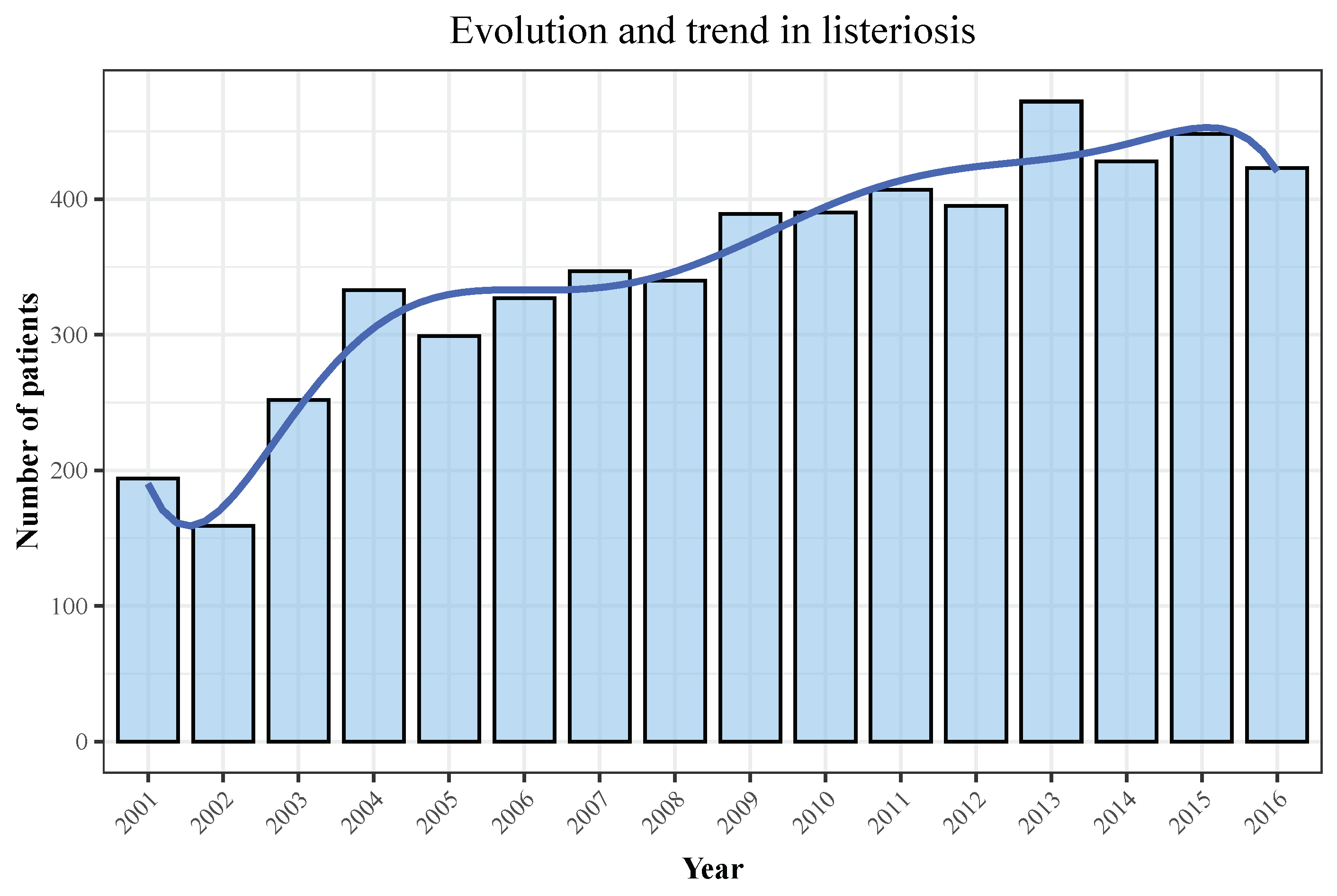
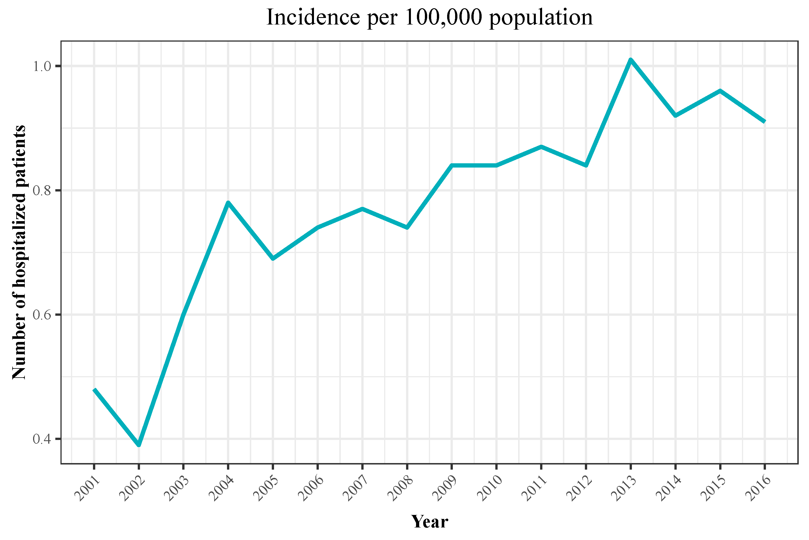
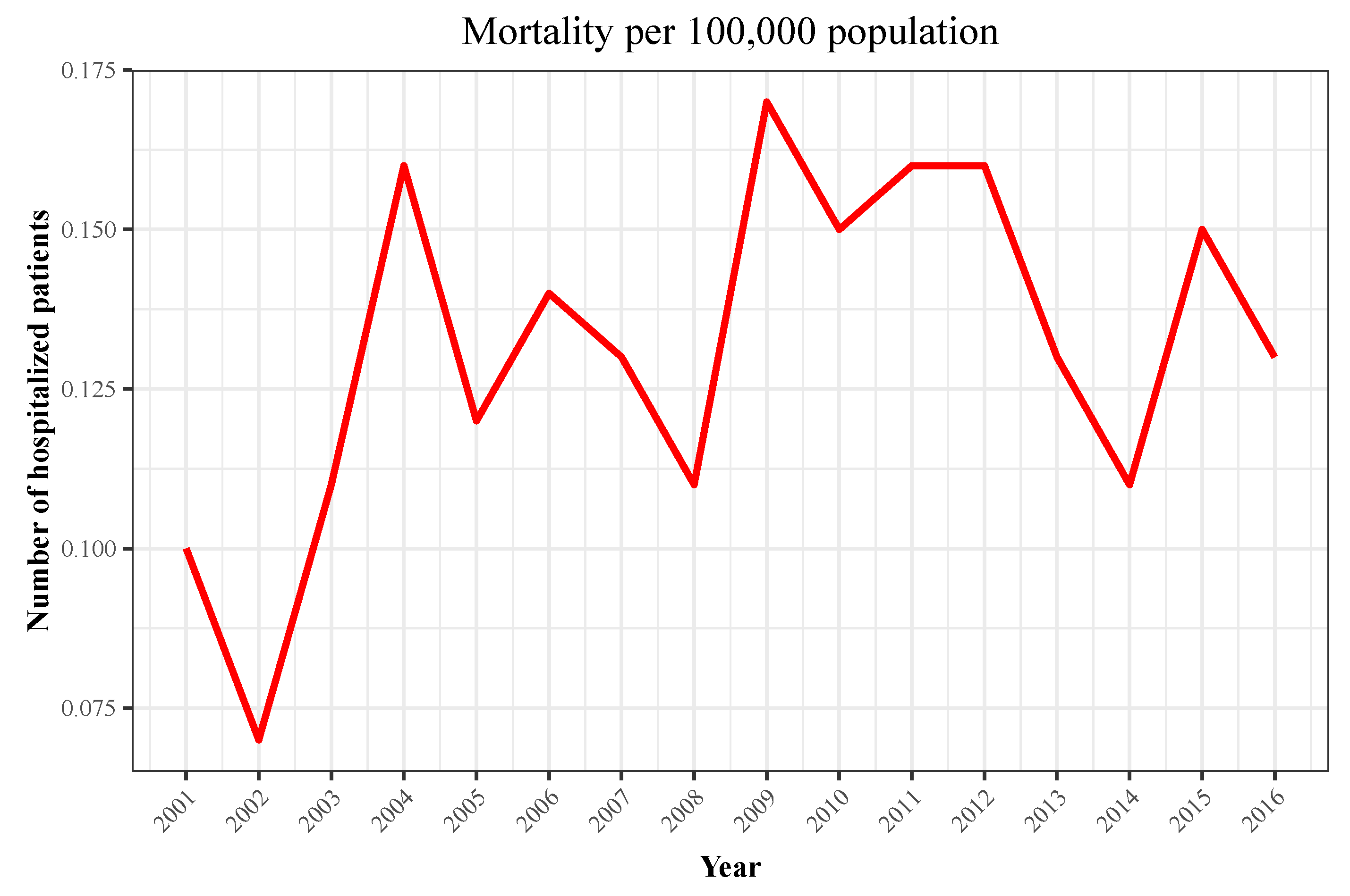
| Year | Hospitalizations | Deaths | Total Population | Incidence | Mortality |
|---|---|---|---|---|---|
| 2001 | 194 | 40 | 40,670,000 | 0.48 | 0.1 |
| 2002 | 159 | 27 | 41,040,000 | 0.39 | 0.07 |
| 2003 | 252 | 45 | 41,830,000 | 0.6 | 0.11 |
| 2004 | 333 | 69 | 42,547,454 | 0.78 | 0.16 |
| 2005 | 299 | 50 | 43,296,335 | 0.69 | 0.12 |
| 2006 | 327 | 60 | 44,009,969 | 0.74 | 0.14 |
| 2007 | 347 | 60 | 44,784,659 | 0.77 | 0.13 |
| 2008 | 340 | 51 | 45,668,938 | 0.74 | 0.11 |
| 2009 | 389 | 77 | 46,239,271 | 0.84 | 0.17 |
| 2010 | 390 | 72 | 46,486,621 | 0.84 | 0.15 |
| 2011 | 407 | 74 | 46,667,175 | 0.87 | 0.16 |
| 2012 | 395 | 73 | 46,818,216 | 0.84 | 0.16 |
| 2013 | 472 | 61 | 46,727,890 | 1.01 | 0.13 |
| 2014 | 428 | 50 | 46,512,199 | 0.92 | 0.11 |
| 2015 | 448 | 70 | 46,449,565 | 0.96 | 0.15 |
| 2016 | 423 | 62 | 46,440,099 | 0.91 | 0.13 |
| Variable | Survivors (n = 4662) | Deaths (n = 941) | p |
|---|---|---|---|
| Sex (female) | 1940 (41.6%) | 378 (40.2%) | 0.433 |
| Age (IQR) | 63.0 (31.0) | 73.0 (19.0) | <0.001 |
| Pregnancy | 301 (6.5%) | 0 (0.0%) | <0.001 |
| Newborn | 273 (5.9%) | 23 (2.4%) | <0.001 |
| Sepsis/septic shock | 409 (8.8%) | 216 (23.0%) | <0.001 |
| Bacteremia | 839 (18.0%) | 124 (13.2%) | <0.001 |
| Endocarditis | 38 (0.8%) | 10 (1.1%) | 0.577 |
| CNS | 1988 (42.6%) | 465 (49.4%) | <0.001 |
| Peritonitis | 153 (3.3%) | 41 (4.4%) | 0.122 |
| Febrile gastroenteritis | 199 (4.3%) | 22 (2.3%) | 0.7 |
| Malignancy | 1054 (22.6%) | 347 (36.9%) | <0.001 |
| CKD | 364 (7.8%) | 109 (11.6%) | <0.001 |
| Cirrhosis of the liver | 581 (12.5%) | 144 (15.3%) | 0.21 |
| Immunosuppression | 1764 (37.8%) | 468 (49.7%) | <0.001 |
| Variable | Survivors (n = 4662) | Deaths (n = 941) | p |
|---|---|---|---|
| Newborn | 276 (5.9%) | 23 (2.4%) | <0.001 |
| 1–10 | 34 (0.7%) | 1 (0.1%) | 0.47 |
| 11–20 | 55 (1.2%) | 5 (0.5%) | 0.112 |
| 21–30 | 223 (4.8%) | 5 (0.5%) | <0.001 |
| 31–40 | 428 (9.2%) | 24 (2.6%) | <0.001 |
| 41–50 | 399 (8.6%) | 58 (6.2%) | 0.17 |
| 51–60 | 675 (14.5%) | 111 (11.8%) | 0.35 |
| 61–70 | 958 (20.5%) | 182 (19.3%) | 0.426 |
| 71–80 | 1054 (22.6%) | 308 (32.7%) | <0.001 |
| >81 | 560 (12.0%) | 224 (23.8%) | <0.001 |
| Variable | OR | 2.5% | 97.5% | p |
|---|---|---|---|---|
| (Intercept) | 0.05 | 0.04 | 0.06 | <0.001 |
| Malignancy | 1.94 | 1.58 | 2.4 | <0.001 |
| Sepsis/septic shock | 3.31 | 2.72 | 4.02 | <0.001 |
| Chronic liver disease | 1.68 | 1.36 | 2.07 | <0.001 |
| Immunosuppression | 1.4 | 1.15 | 1.7 | <0.001 |
| CKD | 1.44 | 1.12 | 1.84 | <0.001 |
| CNS | 1.72 | 1.46 | 2.02 | <0.001 |
| 61–70 | 1.46 | 1.17 | 1.81 | <0.001 |
| 71–80 | 2.48 | 2.04 | 3.01 | <0.001 |
| >80 years | 3.98 | 3.19 | 4.96 | <0.001 |
Publisher’s Note: MDPI stays neutral with regard to jurisdictional claims in published maps and institutional affiliations. |
© 2022 by the authors. Licensee MDPI, Basel, Switzerland. This article is an open access article distributed under the terms and conditions of the Creative Commons Attribution (CC BY) license (https://creativecommons.org/licenses/by/4.0/).
Share and Cite
Garcia-Carretero, R.; Roncal-Gomez, J.; Rodriguez-Manzano, P.; Vazquez-Gomez, O. Identification and Predictive Value of Risk Factors for Mortality Due to Listeria monocytogenes Infection: Use of Machine Learning with a Nationwide Administrative Data Set. Bacteria 2022, 1, 12-32. https://doi.org/10.3390/bacteria1010003
Garcia-Carretero R, Roncal-Gomez J, Rodriguez-Manzano P, Vazquez-Gomez O. Identification and Predictive Value of Risk Factors for Mortality Due to Listeria monocytogenes Infection: Use of Machine Learning with a Nationwide Administrative Data Set. Bacteria. 2022; 1(1):12-32. https://doi.org/10.3390/bacteria1010003
Chicago/Turabian StyleGarcia-Carretero, Rafael, Julia Roncal-Gomez, Pilar Rodriguez-Manzano, and Oscar Vazquez-Gomez. 2022. "Identification and Predictive Value of Risk Factors for Mortality Due to Listeria monocytogenes Infection: Use of Machine Learning with a Nationwide Administrative Data Set" Bacteria 1, no. 1: 12-32. https://doi.org/10.3390/bacteria1010003