Analysis of Wind Power Fluctuation in Wind Turbine Wakes Using Scale-Adaptive Large Eddy Simulation

Abstract

In large wind farms, the interaction of atmospheric turbulence and wind turbine wakes leads to complex vortex dynamics and energy dissipation, resulting in reduced wind velocity and subsequent loss of wind power. This study investigates the influence of vortex stretching on wind power fluctuations within wind turbine wakes using scale-adaptive large eddy simulation. The proper orthogonal decomposition method was employed to extract the most energetic contributions to the wind power spectra. Vertical profiles of mean wind speed, Reynolds stresses, and dispersive stresses were analyzed to assess energy dissipation rates. Our simulation results showed excellent agreement when compared with wind tunnel data and more advanced numerical models, such as the actuator line model and the actuator line model with hub and tower effects. This highlights the important role of coherent and energetic flow components in the spectral behavior of wind farms. The findings indicate a persistent energy cascading length scale in the wake of wind turbines, emphasizing the vertical transport of energy to turbine blades. These results complement existing literature and provide new insights into the dynamics of wind turbine wakes and their impact on wind farm performance.

1. Introduction

In the atmospheric boundary layer with many wind turbines, the interaction of atmospheric turbulence with wind turbine wakes gives rise to intricate and coherent vortices at relatively small scales [1,2,3,4]. The turbulent inflow [5,6] and atmospheric stability [7] strongly influence the complex characteristics of downstream wakes. Moreover, wind turbines reduce the wind speed as they extract kinetic energy from the atmosphere. This effect may reach several kilometers downwind of large wind farms [8]. Wind turbine wakes significantly enhance vortex stretching at hub height, which affects local meteorological conditions [9]. The enhanced atmospheric turbulence leads to strong spatiotemporal fluctuations, which pose a major challenge for wind farm flow control, such as increasing energy extraction and reducing structural load [10]. The impact of atmospheric turbulence on the collective control of wind turbine arrays is known [11].

In turbulence theory, a cornerstone principle is that vortex stretching plays a critical role in spatiotemporal fluctuations while driving the average energy cascade [12,13]. According to D’Alambert’s paradox and the Kutta–Joukowski theorem, the lift on an wind turbine cannot be associated with the restricted Euler dynamics. More specifically, an implication of the circulation conservation in inviscid flow is that the lift generation is associated with the enstrophy production by vortex stretching in the wind farm atmospheric boundary layer [14,15]. This article provides a numerical investigation to clarify the role of vortex stretching and restricted Euler dynamics in wind farm power fluctuations. This effect has not been thoroughly investigated by previous studies [11,13]. Conducting a parametric analysis of the direct effects of vortex stretching on lift generation and wake recovery poses a considerable challenge due to the complexity of the underlying physical mechanisms [16]. For example, the literature disagrees on the deflection or the recovery of wakes due to Coriolis force or mountain waves, respectively [17,18,19]. Recent investigations suggest that the wind power fluctuations follow the $-5/3$ spectrum of inertial range and that the wind-induced structural load on turbines is associated with a time-varying mean wind. The present study thus focuses on the average energy cascade by vortex stretching, (e.g., [12,20]) in large eddy simulation (LES) of wind farms in neutral atmospheric boundary layers, using actuator-disk model of individual wind turbine. In this study, we highlight the fact that the vorticity and the strain are in complementary distribution (e.g., [21]) and consider vortex stretching to represent spatiotemporal fluctuations of subgrid-scale turbulence [20,22].

1.1. Relevant Past Work

Chamorro and Porté-Agel [23] considered a wind tunnel measurement of the wake behind a single model turbine and an array of 30 model turbines placed in a turbulent boundary layer. These experiments used model turbines with rotating blades spanning a rotor diameter of 15 cm. Several studies compared such measurements against LES of wind farms [24]. Bossuyt et al. [10] considered a wind tunnel experiment with 100 porous disks with a diameter of 3 cm as model turbines. Stevens et al. [24] observed that the actuator line method captures the wind turbine wakes better than the actuator disk method. Stevens and Meneveau [5] thoroughly reviewed the wind turbine wakes simulated by various turbine models. Typically, the actuator disk method leads to flattened near wake profiles and sharp deviation from the ground surface. Such deviations are adequately controlled with an actuator line model if the nacelle, rotational effects of turbines, tip vortices, and the atmospheric boundary layer (ABL) region below the rotor bottom are sufficiently resolved [25]. Bossuyt et al. [10] investigated the effects of wake-generated turbulence in the atmospheric boundary layer and observed peaks in the wind power spectrum at dimensionless frequencies $fD/U=1/7$ and $fD/U=1/14$ for staggered and aligned turbine arrangements, respectively. These harmonics correspond to the convective travel time of turbulence structures between rows of turbines in each configuration. Here, D is the turbine diameter and U is the hub-height velocity, which in the present case are $0.15$ m and $2.22$ m/s, respectively. Separating the wake-generated effects from atmospheric turbulence remains an ongoing challenge because surface wake fluctuations and turbulence fluctuations occur at overlapping frequencies.

Moser et al. [26] and Bose and Park [27] provided a general review of various subgrid-scale models and wall-modeled LES. In contrast, Mehta et al. [28] and Sarlak et al. [29] covered a wind turbine wake-related review of LES. Such studies clearly explained various subgrid-scale models, including the standard Smagorinsky model [30], the dynamic Smagorinsky model [31], as well as the dynamic mixed model [32], and their role in affecting flow structures and turbine loading [5]. Mehta et al. [28] suggested that for a fine grid that accurately captures the vorticies, shear layer structures, and the corresponding instabilities, the particular choice of the subgrid model is not a determining factor in LES accuracy [29]. There seems to be a strong need to understand how the coherent vorticies can cause high-frequency structural vibrations and substantial impulsive loads on turbines [33]. More specifically, vortex stretching is a potential framework to represent how upstream wind turbines play a dynamic role in the rapid breakdown of coherent structures in downstream wakes [34].

1.2. Scope and Objective

Wind farms encompass atmospheric turbulence at multiple spatial scales in wind turbine wakes (ranging from 1 to 10 m) to atmospheric motions (in the range of 100 m to several kilometers). It is thus crucial to examine the scale adaptivity of dissipation rates in LES of wind farms in comparison to wind tunnel measurements. Grid-generated turbulence in wind tunnel measurements reveals that vorticity is produced by vortex stretching at a rate three times faster than it dissipates [35]. Here, we compare wind farm LES results with wind tunnel measurements of Chamorro and Porté-Agel [23] for a-posteriori assessment of the correlation between vorticity production by vortex stretching and turbulence dissipation. We compare the dispersive stresses observed in LES results with the Reynolds stresses observed in wind tunnel measurements to evaluate the characteristics of turbulent activity that transfers moment downward in the wind farm boundary layer. We further extend the wind tunnel measurements of Chamorro and Porté-Agel [23] to characterize the time-series of resolved velocity extracted from wind farm LES by separating frequencies with the proper orthogonal decomposition (POD) method. Finally, we show that the LES and the wind tunnel measurement of a model wind farm help understand one of the best known mathematical results regarding the regularity and uniqueness of the velocity field of turbulent flows. Consequently, our investigation hints at the vortex stretching framework for the lift generation mechanism.

Recent work [13,22,36] has focused on developing a scale-adaptive LES method for aerodynamic applications. In the present work, we extend the findings of Stevens et al. [24] and Dai et al. [37] toward understanding a vortex stretching framework for wind farm aerodynamics. However, a full discussion of wind farm layout optimization is outside the scope of this work.

Section 2 provides a brief outline of the LES methodology and the Gaussian actuator disk model. Section 4 summarizes the research findings. Section 5 highlights key findings and outlines some potential future research directions.

2. LES Method and the Gaussian Actuator Disk Model of Wind Farms

2.1. Restricted Euler Dynamics of Velocity Gradient

Under the enstrophy dynamics, lift generation on wind turbine blades is associated with the attachment of leading-edge vortex. As the blade rotates in a wind farm, however, intermittent fluctuations of wind speed are associated with the scale-wise cascade of kinetic energy driven by vortex stretching and the turbulence production of small-scale motions in wind turbine wakes [13,37,38]. One observes from the governing equations of enstrophy $\left({\omega }_i^2\right)$ and strain $\left({\mathcal{S}}_{ij}{\mathcal{S}}_{ij}\right)$ that the enstrophy production by vortex stretching ${\omega }_i{\mathcal{S}}_{ij}{\omega }_j$ is closely related to strain rate self-amplification. The energy transfer mechanism is influenced by the stretching of the vortex and self-amplification of the strain according to the restricted Euler dynamics,

$${\displaystyle \frac{1}{2}}{\displaystyle \frac{D{\omega }_i^2}{Dt}}={\omega }_i{\mathcal{S}}_{ij}{\omega }_j$$

(1)

and

$${\displaystyle \frac{1}{2}}{\displaystyle \frac{D\left({\mathcal{S}}_{ij}{\mathcal{S}}_{ij}\right)}{Dt}}=-{\mathcal{S}}_{ij}{\mathcal{S}}_{jk}{\mathcal{S}}_{ki}-{\omega }_i{\mathcal{S}}_{ij}{\omega }_j.$$

(2)

Clearly, correlations between ${\mathcal{S}}_{ij}$ and ${\omega }_i$ (or ${\mathcal{R}}_{ij}$) play a dynamical role in wind power fluctuations and wind-induced load on blades. Equations (1) and (2) provide a keystone principle of modern turbulence theory for the design and control of wind farms [12]. The rate of production of total strain $\sqrt{{\mathcal{S}}_{ij}{\mathcal{S}}_{ij}}$ via strain self-amplification is given by three real eigenvalues of strain tensor, ${\lambda }_1>{\lambda }_2>{\lambda }_3$, where

$${\mathcal{S}}_{ij}{\mathcal{S}}_{jk}{\mathcal{S}}_{ki}=-2{\lambda }_1{\lambda }_2{\lambda }_3$$

and ${\lambda }_1+{\lambda }_2+{\lambda }_3=0$ (due to incompressibility). According to Equation (1), local enstrophy is increased and strain is decreased when the vorticity vector aligns more with the strain-rate eigenvectors with positive eigenvalues. Thus, vortex stretching and strain self-amplification would naturally strengthen the velocity gradients via nonlinear self-advection ($\mathit{u}·\nabla \mathit{u}$). The restricted Euler dynamics of velocity gradients shows that total strain $\sqrt{{\mathcal{S}}_{ij}{\mathcal{S}}_{ij}}$ cannot adequately represent the energy transfer rate associated with filtered nonlinear advection ($\mathit{u}·\nabla \mathit{u}$) in the inertial range turbulence without considering vortex stretching.

2.2. The Large Eddy Simulation Framework

In LES of turbulent flows, filtering the fluctuating motion leads to the residual stress ${\tau }_{ij}={\overline{u_{i}u}}_j-{\overline{u}}_i{\overline{u}}_j$, where $\overline{(·)}$ denotes a filtering operation. Motivated by the aforementioned discussion, an interpretation of the inherent dynamical features of the residual stress ${\tau }_{ij}$ are correlated with interactions between the strain rate (${\mathcal{S}}_{ij}{\mathcal{S}}_{ij}$) and the enstrophy (${\omega }_i^2$) [20,21]. Applying a filter to the continuity and momentum equations, we have

$${\displaystyle \frac{𝜕{\overline{u}}_i}{𝜕x_i}}=0,$$

(3)

$${\displaystyle \frac{𝜕\overline{u_i}}{𝜕t}}+{\overline{u}}_j{\displaystyle \frac{𝜕{\overline{u}}_i}{𝜕x_j}}=-{\displaystyle \frac{𝜕\overline{p}}{𝜕x_i}}-{\displaystyle \frac{𝜕{\tau }_{ij}}{𝜕x_j}}+f_i\chi (\mathit{x},t),$$

(4)

where, ${\overline{u}}_i$ denotes the filtered velocity components, $({\overline{u}}_1,{\overline{u}}_2,{\overline{u}}_3)=(\overline{u},\overline{v},\overline{w})$ in the streamwise ($x=x_1$), spanwise ($y=x_2$) and surface-normal directions ($z=x_3$), respectively. The function $\chi (\mathit{x},t)$ becomes 0 in the fluid and 1 on the immersed solid. In the Smagorinsky model,

$${\tau }_{ij}-{\displaystyle \frac{1}{3}}{\tau }_{kk}{\delta }_{ij}=-2c_k{\mathsf{\Delta }}_{\mathrm{les}}^2\sqrt{2{\mathcal{S}}_{ij}{\mathcal{S}}_{ij}}{\mathcal{S}}_{ij},$$

(5)

where, $c_k(\mathit{x},t)$ is the model parameter that depends locally on the flow conditions. The term $\sqrt{2{\mathcal{S}}_{ij}{\mathcal{S}}_{ij}}$ in the model represents the kinetic energy dissipation. In the dynamic Smagorinsky approach, $c_k(\mathit{x},t)$ is dynamically adjusted to account for the local production of enstrophy by vortex stretching. This adaptation ensures that the model captures the varying turbulent characteristics across different regions of the flow field.

2.3. Vortex-Stretching-Based Scale-Adaptive Subgrid Model

In the present study, we approximate the daviatoric part of ${\tau }_{ij}$ as

$${\tau }_{ij}-{\displaystyle \frac{1}{3}}{\tau }_{kk}{\delta }_{ij}=-2c_k{\mathsf{\Delta }}_{\mathrm{les}}\sqrt{k_{\mathrm{sgs}}}{\mathcal{S}}_{ij}.$$

(6)

Comparing Equation (5) with Equation (6) provides the widely used Smagorinsky model $k_{\mathrm{sgs}}=2{\mathsf{\Delta }}_{\mathrm{les}}^2{\mathcal{S}}_{ij}{\mathcal{S}}_{ij}$ [30]. However, Deardorff [39] proposed to use Equation (6) by solving a transport equation to approximate $k_{\mathrm{sgs}}$ appearing in Equation (6).

In the present study, we consider the resolved (or Leonard) stress ${\tau }_{ij}^L=\widetilde{{\overline{u}}_i{\overline{u}}_j}-\widetilde{{\overline{u}}_i}\widetilde{{\overline{u}}_j}$ to approximate $k_{\mathrm{sgs}}$ without solving any transport equation; see [13,22]. Vortex stretching and strain-rate self-amplification dictate the energy cascade [12,13,20,40]. We connect the energy cascade mechanism to the deviatoric part of the Leonard stress, resulting in the following expression:

$${\tau }_{ij}^{L^{dev}}{\tau }_{ji}^{L^{dev}}={\displaystyle \frac{1}{2}}\left[{\mathcal{S}}_{ij}{\omega }_j{\mathcal{S}}_{ik}{\omega }_k+{\displaystyle \frac{1}{3}}{\left({\mathcal{G}}_{ij}{\mathcal{G}}_{ji}\right)}^2\right],$$

(7)

where, the superscript ${(·)}^{dev}$ represents the deviatoric part of the (Leonard) stress. Using Equation (7) and dimensional analysis, we can find the following expression [13,41]:

$$k_{\mathrm{sgs}}={\displaystyle \frac{{\mathsf{\Delta }}_{\mathrm{les}}^2{\left(\frac{1}{2}{\mathcal{S}}_{ij}{\omega }_j{\mathcal{S}}_{ik}{\omega }_k+\frac{1}{6}{({\mathcal{G}}_{ij}{\mathcal{G}}_{ji})}^2\right)}^3}{{\left[{\left({\mathcal{S}}_{ij}{\mathcal{S}}_{ij}\right)}^{5/2}+{(\frac{1}{2}{\mathcal{S}}_{ij}{\omega }_j{\mathcal{S}}_{ik}{\omega }_k+\frac{1}{6}{({\mathcal{G}}_{ij}{\mathcal{G}}_{ji})}^2)}^{5/4}\right]}^2}}.$$

(8)

Few previous studies considered Equation (8) to provide a numerical model of the turbulence eddy viscosity ${\nu }_{\tau }=c_k{\mathsf{\Delta }}_{\mathrm{les}}\sqrt{k_{\mathrm{sgs}}}$, which accounts for magnitudes of the vortex stretching vector and the strain-rate tensor. This study is the first-time analysis of such a scale-adaptive LES framework with respect to wind tunnel measurements. For $0.3<c_k<0.4$, the scale-adaptive model provides a dissipation rate similar to that predicted by the Smagorinsky model for decaying isotropic turbulence. The model’s performance is then tested with $c_k=0.325$ for channel flow [42], wind farms over forests [43], and wind farms over complex terrain [41].

2.4. Wind Turbine Parametrization

Horizontal axis wind turbines are optimized lift machines. The actuator disk theory assumes that the fluid flow around a wind turbine is steady (wind does not change in time), stationary (no lift forces), inviscid (viscous losses are neglected), and irrotational (prohibits the generation of vorticity). Under these assumptions, a horizontal axis wind turbine is simulated as a force acting over an area that the blades sweep during one rotation. In momentum Equation (4), the body force for wind turbine takes the following form:

$$f_i\chi (\mathit{x},t)=-{\displaystyle \frac{1}{2}}\rho c_t{u}_d^2{A}_c{\delta }_{i1}\chi (\mathit{x},t).$$

(9)

Here, $u_d$ is the magnitude of the relative velocity projected onto the area swept by a turbine [24]. In the rest of the article, this formulation is referred to as the “classical ADM”.

Similar to the actuator disk model with rotation (ADM-R), the Gaussian actuator disk model (G-ADM) accounts for both the axial and the tangential forces. The rotor swept area is simulated as a collection of lines from the center to the edge of the rotor disk. Each line is discretized as a collection of elements in plane polar coordinates. The force is scaled by a solidity factor $\varphi$ (the ratio of the volume occupied by three blades to the total rotor volume). The lift and the drag on each grid point are calculated on the basis of the projected wind speed and angle of attack. These forces are then projected on the flow field through the Gaussian function [44]:

$$f_i\chi (\mathit{x},t)={\displaystyle \frac{F_i}{\sqrt{2\pi }{\mathsf{\Delta }}_G}}exp\left(-{\displaystyle \frac{1}{2}}{\displaystyle \frac{{\left|\mathit{r}\right|}^2}{{\mathsf{\Delta }}_G^2}}\right),$$

(10)

where, $\mathit{r}=\mathit{x}-\mathit{c}$, the center of the Gaussian is $\mathit{x}=\mathit{c}$, and $F_i$ includes the lift ($F_l$) and the drag ($F_d$) given by

$$F_l=\varphi {\displaystyle \frac{1}{2}}{c}_l\left(\alpha \right)\rho u_d^2{A}_w\mathrm{and}{F}_d=\varphi {\displaystyle \frac{1}{2}}{c}_d\left(\alpha \right)\rho u_d^2{A}_w.$$

Coefficient $1/\left(\sqrt{2\pi }{\mathsf{\Delta }}_G\right)$ is chosen to ensure that the integral of the Gaussian (with respect to $\left|\mathit{r}\right|$) becomes 1. Each airfoil is associated with a lookup table that provides the lift and drag coefficients as a function of the angle of attack ($\alpha$). The Gaussian (Equation (10)) is considered at each actuator element. The summation of the projected force leads to a collection of a sphere-like region of the body force. Numerical tests suggest that the Gaussian actuator disk model approaches the actuator line model if the grid is refined while satisfying ${\mathsf{\Delta }}_G>2{\mathsf{\Delta }}_{\mathrm{les}}$. Moreover, the Gaussian actuator disk model is less sensitive to the grid spacing and ${\mathsf{\Delta }}_G$ with respect to the actuator line model considering the same Gaussian projection of the force; see [44].

While the Gaussian actuator disk model (G-ADM) introduces other effects by mimicking tangential forces and rotational effects, it remains computationally efficient for capturing large-scale wind farm interactions and mesoscale phenomena. However, it misses localized flow features such as tip and hub vortices, as it typically uses only 5–10 grid points for the rotor disk. In contrast, the actuator line model, which requires 30–40 actuator points per blade, offers a more accurate representation of individual blade dynamics and wake interactions, although at a higher computational cost; see [45]. Additionally, all wind turbine models experience force projection function errors, whether they are based on the actuator disk, actuator line, or advanced actuator line model.

3. Numerical Method and Computational Setup

We utilized an “in-house” LES code that solves the filtered Navier–Stokes equations using the finite volume method [22,36,43]. The material derivative of the filtered Navier–Stokes equations is discretized using a symmetry-preserving numerical scheme, ensuring the preservation of small-scale turbulence and energy conservation [46,47]. The bottom surface is parameterized using a “canopy-stress” boundary condition, which relates the local velocity to the wall-shear stress at the surface (first grid point $z_1$) as $\sqrt{\tau }=c_d\tilde{u}\left(z\right)$, where $c_d=k^2/ln{(z_1/z_0)}^2$ is the drag coefficient [13,43]. Lateral boundary conditions are set as periodic, and the atmosphere is modeled using a slip boundary condition.

At the inlet plane ($x=x_{\min }$), synthetic turbulence is generated using stochastic forcing applied to linearized two-dimensional Navier–Stokes equations. Perturbations $\langle 0,v^{\prime }(0,y,z,t),w^{\prime }(0,y,z,t)\rangle$, derived from solving the linearized equations, are introduced as fluxes at the inlet, propagating into the three-dimensional fluid domain. These perturbations are superimposed onto the classical logarithmic undisturbed mean velocity profile, resulting in an inflow condition of $\langle U\left(z\right),v^{\prime }(0,y,z,t),w^{\prime }(0,y,z,t)\rangle$, where $U\left(z\right)=u_{\ast }/k(ln(z/z_0))$ [13,41,43].

In this study, we consider two cases: an isolated rotor and a wind farm consisting an aligned $10\times 3$ array of turbines immersed in a neutral atmospheric boundary layer. Figure 1 illustrates the computational domain: (a) the $36D\times 6D\times 3D$ domain for LES of a single turbine and (b) the $96D\times 12D\times 4.5D$ domain for the $10\times 3$ wind farm array. The rotor diameter and the hub height of each turbine are $0.15$ m and $0.125$ m, respectively.

4. Result Analysis

The validation of LES results against experimental data has been considered in several recent studies. Examples include comparisons of wind turbine wake simulations using different LES frameworks [48,49]. This section considers two wind tunnel measurements: one is for an isolated wind turbine and the other is for a $10\times 3$ array wind turbine [23,50]. For a single turbine (e.g., Figure 1a), the velocity data are collected on eight vertical lines in the vertical mid-plane. The location of these lines are indicated by $x/D=-1$, $x/D=2$, $x/D=3$, $x/D=5$, $x/D=7$, $x/D=10$, $x/D=14$, $x/D=20$, where $x/D=0$ refers to the location of the turbine. Similarly for the wind farm simulation, the velocity data were collected in the vertical mid-plane passing through the central column of the array. The streamwise location of a row of the farm is denoted by $X_d$ such that $X_d=0$ refers to the first row. At the wake behind each row, we considered four streamwise locations. These locations were denoted by local distances $x/D=0$, $x/D=1$, $x/D=2$, $x/D=3$, and $x/D=4$, where $x/D=0$ refers to the corresponding row. Finally, we considered a set of n points ${\left\{{\mathit{x}}_d\right\}}_{d=1}^n$, where we captured instantaneous velocity $u_i({\mathit{x}}_d,t)$ for POD analysis. Here, $i=1,2,3$ corresponds to streamwise, spanwise, and wall-normal velocities, respectively.

To test the sensitivity of mesh resolution, we considered different cases ranging from very coarse to fine mesh resolutions.

Table 1. Numerical setup of all the cases used in the large eddy simulations with different grid resolutions for the G-ADM wind turbine model. Cases M1 to M5 correspond to LES of a single wind turbine, while cases WF1, and WF2 correspond to LES of a wind farm. Here, $\mathsf{\Delta }={\left(\mathsf{\Delta }x\mathsf{\Delta }y\mathsf{\Delta }z\right)}^{1/3}$. $N_{x_2}$ and $N_{x_3}$ represent the number of grid points across the rotor along the spanwise and surface-normal directions.

Cases	Resolution	${\mathit{N}}_{{\mathit{x}}_2}$	${\mathit{N}}_{{\mathit{x}}_3}$	$\mathsf{\Delta }/\mathit{D}$
M1	$48\times 9\times 16$	1	5	$0.45$
M2	$64\times 16\times 24$	3	8	$0.29$
M3	$128\times 21\times 36$	3	12	$0.18$
M4	$180\times 30\times 48$	5	16	$0.13$
M5	$324\times 56\times 72$	9	24	$0.079$
WF1	$476\times 60\times 72$	5	16	$0.13$
WF2	$1024\times 128\times 96$	10	32	$0.065$

presents the set-up of seven test cases (M1–M5) for a single turbine and two test cases (WF1 and WF2) for an array of 30 wind turbines. This analysis considers an average grid spacing $\mathsf{\Delta }/D$ that varies in the range from 0.079 to 0.45.

Figure 2 shows the wake and vortex system created by the Gaussian actuator disk model. Compared to the wakes predicted by the actuator line model (e.g., [29]), these isosurface plots of vorticity $\left|\mathsf{\omega }\right|$ indicate that the Gaussian actuator disk model marginally resolves the tip vortices in the near wake, whereas the far wake vortices are distorted. The vortices captured with the present LES appear less resolved compared to what would have been captured with the actuator line model (e.g., [29]). The figure illustrates isosurface plots of the vorticity magnitude $\left|\mathsf{\omega }\right|$ in the case of a wind farm. In these wind farm scenarios, a distorted vorticity field is observed after the first row of turbines. When wind turbines are deployed in large arrays of utility-scale turbines, their efficiency is influenced by the interaction between the vorticity-dominated wake and the atmospheric boundary layer (e.g., [1]). We discuss these effects in the next two sections.

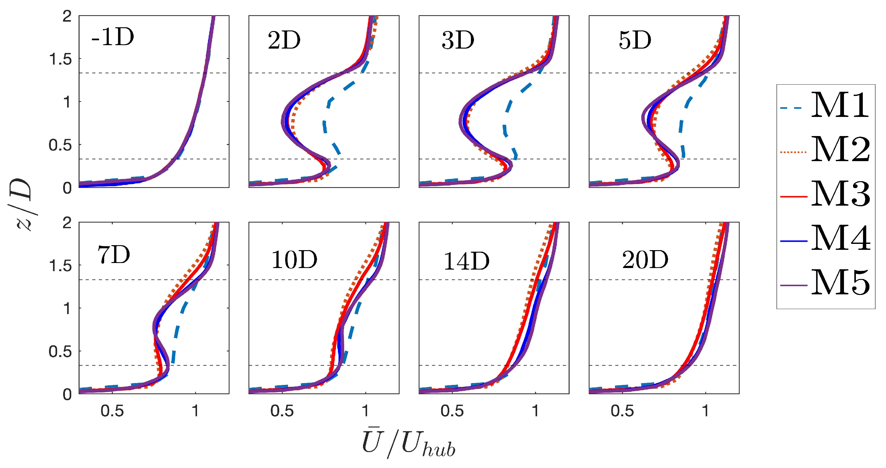
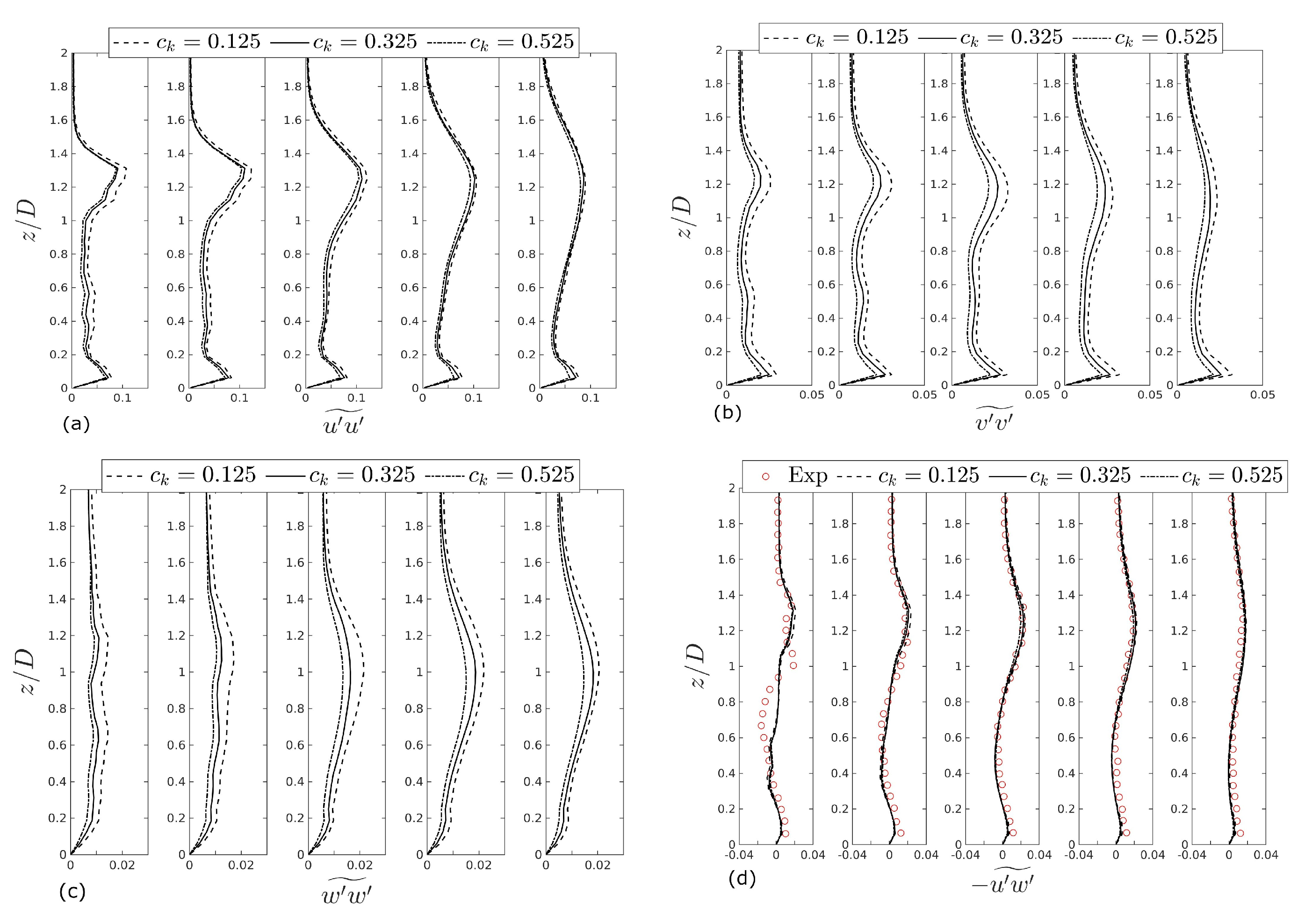
4.1. Mesh Sensitivity Analysis

To test the sensitivity of mesh resolution, we consider different cases ranging from very coarse to fine mesh resolutions. Table 1 presents the set-up of 7 test cases (M1–M5) for a single turbine and 2 test cases (WF1 and WF2) for an array of 30 wind turbines. This analysis considers an average grid spacing $\mathsf{\Delta }/D$ that varies in the range from 0.079 to 0.45.

Figure 2 shows the wake and vortex system created by the Gaussian actuator disk model. Compared to the wakes predicted by the actuator line model e.g., [29], these isosurface plots of vorticity $\left|\mathbf{\omega }\right|$ indicate that the Gaussian actuator disk model marginally resolves the tip vortices in the near wake, whereas the far wake vortices are distorted. The vortices captured with the present LES appear less resolved compared to what would have been captured with the actuator line model e.g., [29]. The figure illustrates isosurface plots of the vorticity magnitude $\left|\mathbf{\omega }\right|$ in the case of a wind farm. In these wind farm scenarios, a distorted vorticity field is observed after the first row of turbines. When wind turbines are deployed in large arrays of utility-scale turbines, their efficiency is influenced by the interaction between the vorticity-dominated wake and the atmospheric boundary layer e.g., [1]. We will discuss these effects in the next two sections.

Relatively few of the past CFD investigations considered the detailed dynamics of the atmospheric boundary layer containing turbine-like obstacles; see [5,51]. The current investigation provides some further insight into the local dynamics of wind turbine wakes. Figure 3 shows the vertical profiles of the streamwise velocity at eight locations for a single wind turbine. These velocity profiles represent five test cases, where five meshes are considered for G-ADM turbine model. For relatively coarse meshes, e.g., $48\times 9\times 16$ and $64\times 16\times 24$, the numbers of grid points ($N_{x_3}$) across the rotor disk in the vertical direction are $N_{x_3}=5$ and $N_{x_3}=8$, respectively. The numbers of grid points in the streamwise horizontal direction are $N_{x_2}=1$ and $N_{x_2}=3$, respectively. The velocity profiles predicted on these two coarse grids disagree in the near wake region; however, they predict the far wake profile (for $x/D>10$) relatively accurately. Increasing the number of grid points in the vertical direction to $N_{x_3}=12$ (M3) provides the wind profiles that are insensitive to a further grid refinement. In this case, the ratio of the horizontal grid spacing to the vertical grid spacing is 4:1.

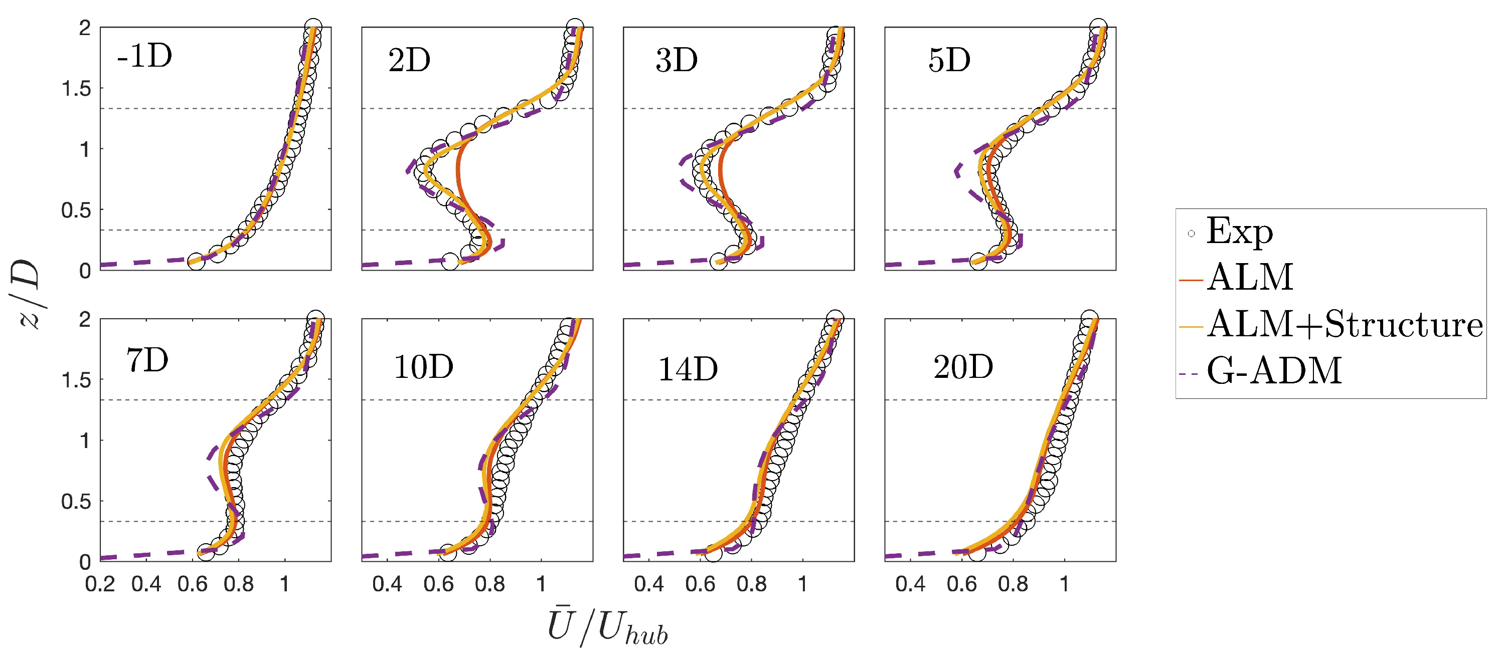
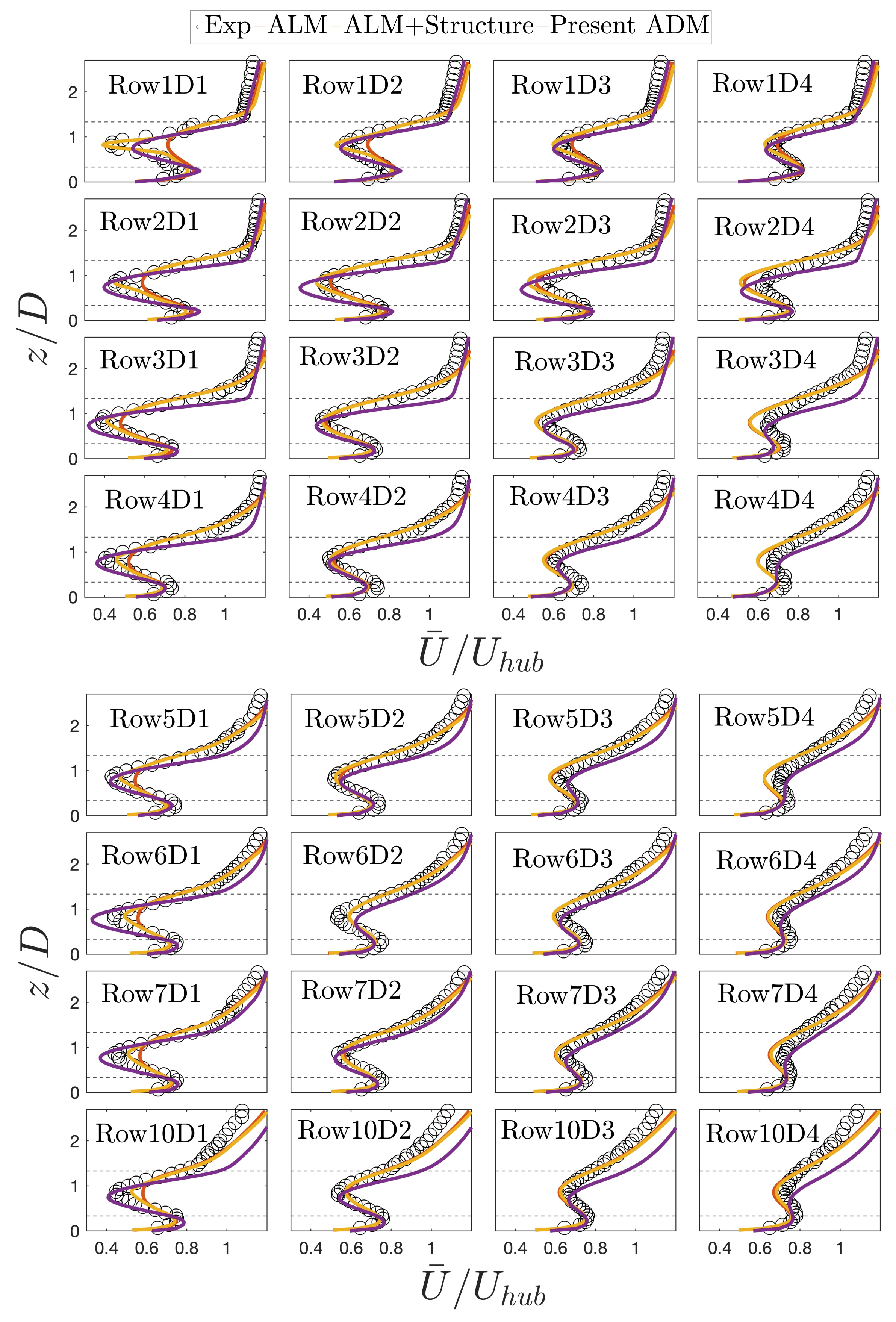
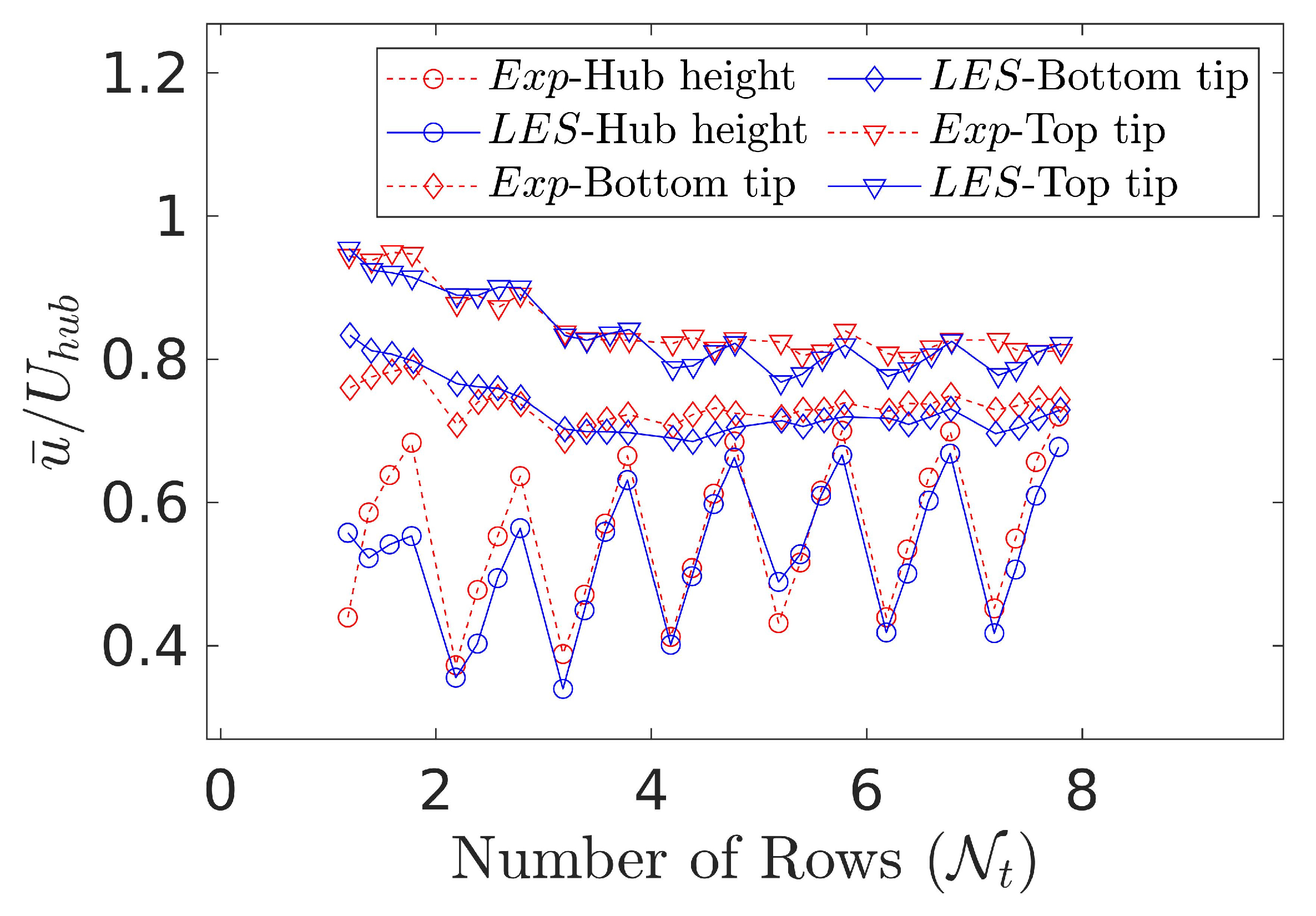
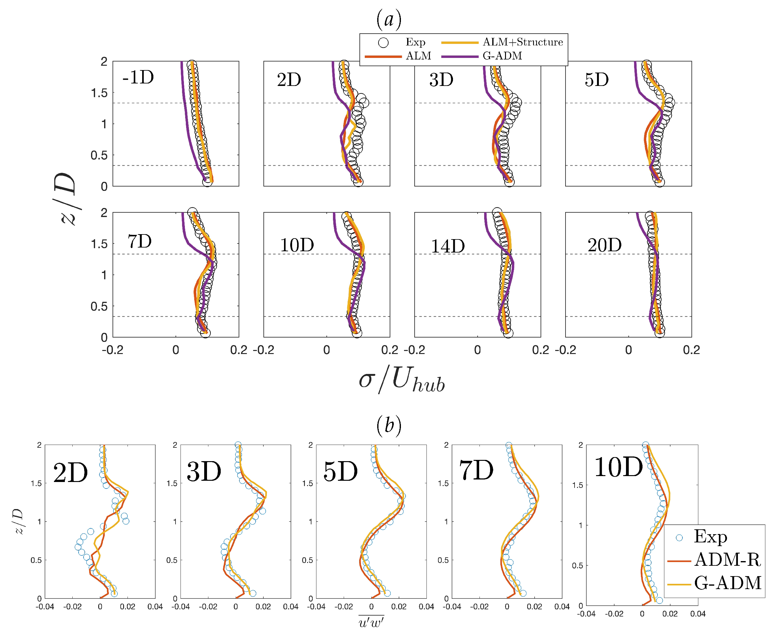
Comparison of LES Results Against Wind Tunnel Measurements

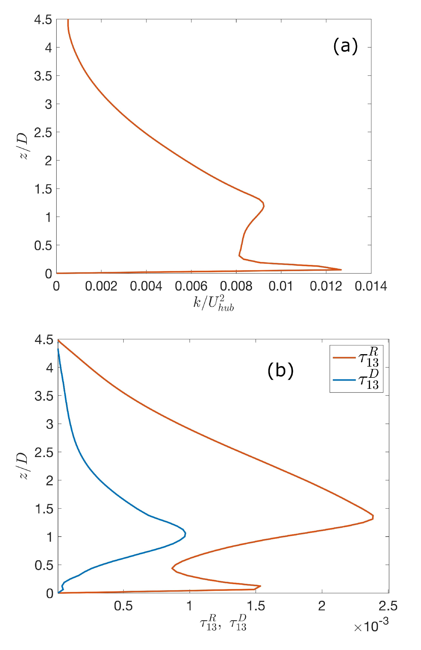
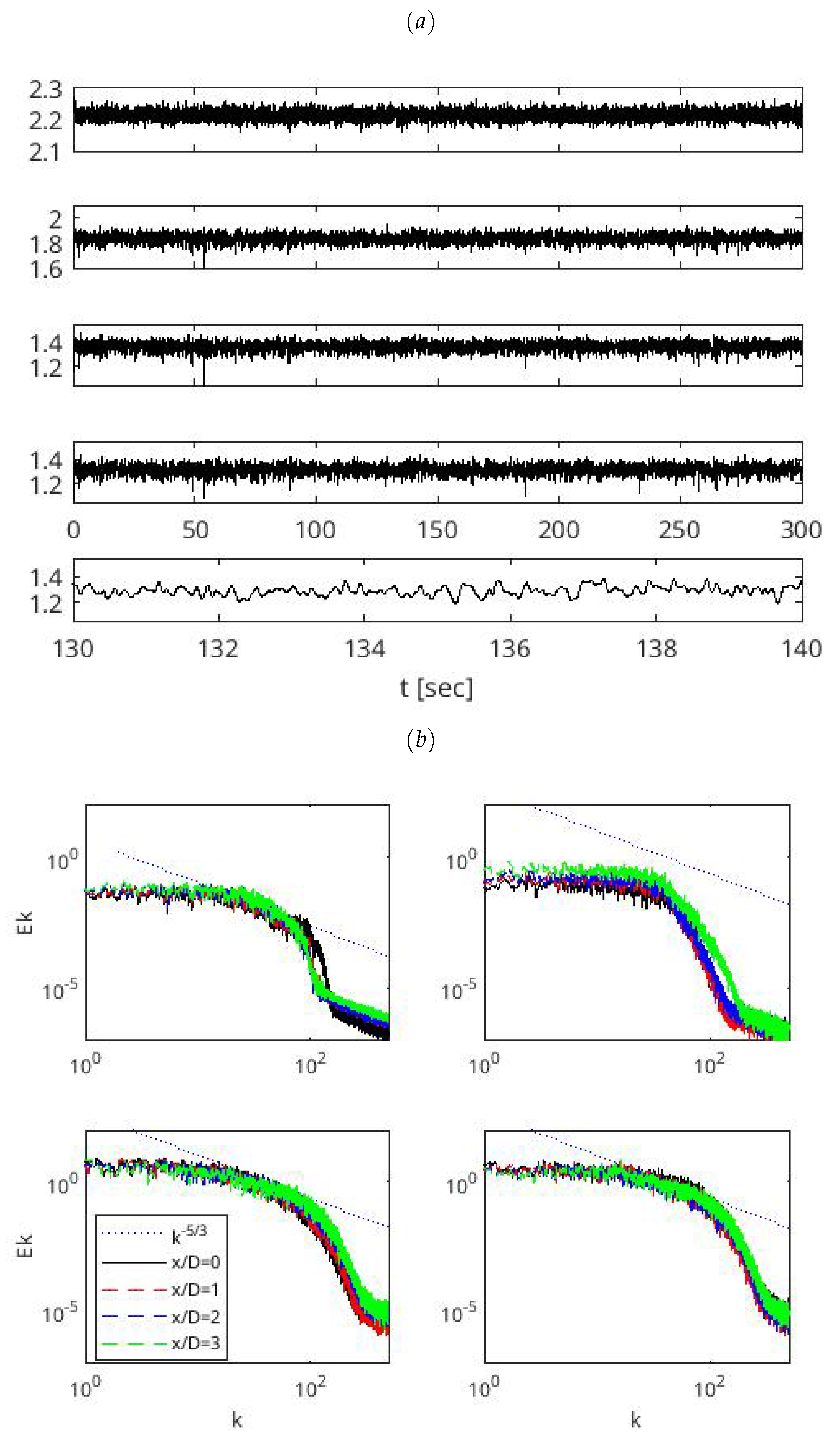
At the wake of an isolated wind turbine, Figure 4 compares the vertical profiles of the mean streamwise velocity against wind tunnel measurements [23]. Additionally, we considered the LES data provided by Stevens et al. [24] to test G-ADM against more expensive wind turbine models such as the actuator line and the actuator line plus structure. Here, “structure” refers to the tower and hub of the wind turbine. LES studies using the classical ADM were considered in several previous investigations [25,52,53,54,55,56]. Utilizing G-ADM for the wind turbine, the outcomes of our scale-adaptive LES agree well with the reference LES data from Stevens et al. [24]. In both the near-wake ($x/D<5$) and far-wake regions ($x/D\ge 5$), the velocity predictions with G-ADM appear very similar to those of experiments.

The scale-adaptive LES method accounts for the vortex interaction between the resolved and unresolved fields while simultaneously using the strain and the vorticity fields according to the subgrid-scale model Equation (8). As the wind farm becomes larger and larger, the turbulence mixing caused by such a vorticity field may significantly alter the flow structures by enhancing the vertical transport of momentum [1,4,57]. Vertical profiles of the mean streamwise velocity $\overline{u}\left(z\right)$ indicate the rate of dissipation per unit mass $ϵ\left(z\right)=-\widetilde{u^{\prime }{w}^{\prime }}𝜕\overline{u}/𝜕z$. Indicating the position of each row of the wind farm by $x/D=0$, Figure 5 shows the vertical distribution of velocity $\overline{u}\left(z\right)$ in the vertical mid-plane at four locations, $x/D=1,2,3,4$, in the wake behind each row. The velocity profiles predicted by the Gaussian actuator disk model have shown excellent agreement with the experimental results and corresponding LES data. When the Gaussian actuator disk model was used, the thrust coefficients for each turbine were locally evaluated at each actuator point. In current simulations, lift and drag coefficients were approximated and injected manually into the LES code.

Figure 6 illustrates the effects of the wind farm on the vertical profiles of the atmospheric boundary layer wind. For clarity, Figure 6a shows the wind profile at the inlet and Figure 6b compares the velocity profiles in the wakes of fourth, fifth, and sixth rows at the location of $x/D=2$. Figure 6c compares the velocity deficits (differences between the data of Figure 6a,b). Using a curve-fitting algorithm, it was found that the velocity deficit agrees very well with a Gaussian distribution. The results also indicate that the flow within the wind farm reaches an equilibrium state.

To illustrate the gradual decrease in the aerodynamic power available to each turbine, Figure 7 shows the mean streamwise velocity $\overline{u}\left(z\right)$ for three values of z: at the top tip, hub height, and bottom tip of wind turbines. The aerodynamic power of each turbine is proportional to the third power of the velocity. Thus, a comparison of the wind speeds predicted by the LES method with the wind tunnel measurements validates the trend of the energy predicted by our numerical wind farm. Figure 7 shows that streamwise velocities on corresponding locations agree with the experimental data. In addition to indicating the trend of decline of the aerodynamic power, the results depicted in Figure 7 also represent an equivalent trend shown in other field measurements such as the “Invenergy Vantage wind farm” in the state of Washington, USA (see Figure 5 of [55]).

4.2. Turbulence

In this section, we discuss a fundamental question regarding the conceptual foundation of the accuracy of LES and the consideration of LES in wind engineering application. Many aspects of atmospheric turbulence in the atmosphere–wind farm interactions are not adequately analyzed. Of particular interest is how turbulence mixing transports the kinetic energy from the “raw” wind energy resource (the free atmosphere) to heights where wind turbines operate (and other built terrain resides). A fundamental measure of the energy entrainment by turbulence is the fraction of the turbulence kinetic energy captured in the resolved Reynolds stress ${\tau }_{ij}^R$.

To clarify this point, it is necessary to write down the Reynolds decomposition of the resolved velocity ${\overline{u}}_i(\mathit{x},t)={\tilde{u}}_i+u_i^{\prime }(\mathit{x},t)$ and the Reynolds stress, ${\tau }_{ij}^R=\widetilde{u_i^{\prime }{u}_j^{\prime }}$. Here, ${\overline{u}}_i(\mathit{x},t)$ is the “resolved portion” of the actual velocity $u_i(\mathit{x},t)$ of the turbulent flow under consideration. We consider such a decomposition over a time interval consisting of several eddy turnover units so that a further increase in the averaging window does not alter ${\tilde{u}}_i\left(\mathit{x}\right)$. The resolved Reynolds stress measures the portion of the turbulence stress captured with LES. The ratio ${\tau }_{ii}/({\tau }_{ii}^R+{\tau }_{ii})$ estimates the effective resolution of LES. Needless to say, even though computer power has significantly increased, resolving $80\%$ of the energy is a computationally challenging task.

We compared the wind-tunnel measurements of ${\tau }_{ij}^R$ with the corresponding LES results and experimental data. Figure 8a shows the streamwise component of turbulence intensity $\sigma /U_{hub}$ (where $\sigma =\sqrt{{\tau }_{11}^R}$) in the wake of an isolated wind turbine at selected locations of $x/D=2$, $x/D=3$, $x/D=4$, $x/D=5$, $x/D=7$, $x/D=10$, and $x/D=14$. Figure 8b presents the vertical profiles of the resolved shear stress ${\tau }_{13}^R=-\widetilde{u^{\prime }{w}^{\prime }}$. The agreement between the experimental and LES profiles makes it clear that changes in the representation of either the turbine or the subgrid-scale turbulence slightly alter the prediction of the Reynolds stress. However, we observe that the shear stress retains a positive value at the top tip of the wind turbine, regardless of the change in schemes. Thus, the shear production of turbulence in that region entrains high momentum air parcels from aloft and transmits them to the blades; see also [1]. On the other hand, the shear stress is negative below the hub height. Thus, horizontal fluctuations correlate highly with adverse perturbations of vertical velocity near the bottom tip of turbines, $z/D=0.3$. In other words, the LES method captures the accurate unresolved dynamics subject to a sensitivity of schemes.

In Figure 8, one notices that the range of locations $2<x/D<7$ corresponds to a critical region, where a downwind turbine experiences the most of the loads of upwind turbines in an actual wind farm. In this region, the maximum enhancement of turbulence intensity seems to be at the top of the wind turbine (i.e., $z/D\approx 1.3$). This result is also consistent with other findings appearing in experimental investigations [24,53]. Numerical sensitivity of the results is clear from the similar trend of reaching the maximum value in each of the numerical models considered here. However, they differ considerably in capturing the vertical distribution of turbulence intensity due to associated assumptions of the corresponding model. LES results using the Gaussian actuator disk model show a good agreement with the wind tunnel data and corresponding LES data. These observations suggest that a surrogate technique (such as machine learning) might extract the coherent structures captured by LES.

Figure 9a,b show the spatially averaged vertical profiles of the turbulence kinetic energy $k=(1/2)\mathrm{Tr}\left({\tau }_{ij}^R\right)$, the Reynolds shear stress (${\tau }_{13}^R$), and the dispersive shear stress (${\tau }_{13}^D$). The results show that dispersive stresses account for a maximum of $40\%$ of the total stresses in the wind farm. This observation is aligned with the findings of Poggi et al. [58] and Calaf et al. [1].

According to Chamorro and Porte-Agel [50], turbulent flow in wind farms can have two distinct regions based on the downstream distance needed to reach equilibrium. Region-I ($z/D<1.34$) is slightly below the top tip of the wind turbine, which may directly influence the wind turbines’ performance. On the other hand, Region-II ($z/D>1.34$) is slightly above the wind turbine’s top tip. We collected the instantaneously resolved velocity ${\overline{u}}_1(\mathit{x},t)$ at $x/D=3$ in regions of the top tip and the bottom tip, respectively, for each wind turbine. Figure 10 shows the probability density function of normalized ${\overline{u}}_1(\mathit{x},t)$ in Region-I and Region-II. Figure 10a,b in the top row reveal that the flow in Region-I reaches equilibrium from the fourth row, suggesting that turbulence leads to a quick adjustment of the flow within the wind farm. Figure 10c,d in the bottom row illustrate the PDF of the streamwise velocity at the top tip (i.e., Region-II), showing a more gradual adjustment of the flow above the turbine tip height. However, an equilibrium state is reached far downstream (6th–7th row) in the wind farm. This observation indicates that various dynamical processes, such as mixing and vertical transport, occur in these two regions. This observation is also consistent with the experimental prediction of Chamorro and Porte-Agel [50].

The overall subgrid-scale dissipation rate of the vortex stretching-based LES can be related to the dissipation that would have occurred if the Smagorinsky model was used, which leads to $c_k=c_s^2\langle \sqrt{2{\mathcal{S}}_{ij}{\mathcal{S}}_{ij}}\rangle /\langle \sqrt{k_{\mathrm{sgs}}}/{\mathsf{\Delta }}_{\mathrm{sgs}}\rangle$. Using the analytical estimate for the Smagorinsky constant, $c_s=0.18$, we see that the dissipation time scale $\sqrt{2{\mathcal{S}}_{ij}{\mathcal{S}}_{ij}}$ of the Smagorinsky model is 10 times larger than that $\sqrt{k_{\mathrm{sgs}}}/{\mathsf{\Delta }}_{\mathrm{les}}$ of the vortex stretching-based model if $c_k=0.325$. Here, we briefly evaluate the sensitivity of parameter $c_k$ appearing in the subgrid-scale model, Equation (6), of the scale-adaptive LES method. Figure 11 shows the diagonal components of the resolved Reynolds stresses: (a) ${\tau }_{11}^R=-\widetilde{u^{\prime }{u}^{\prime }}$, (b) ${\tau }_{22}^R=-\widetilde{v^{\prime }{v}^{\prime }}$, (c) ${\tau }_{33}^R=-\widetilde{w^{\prime }{w}^{\prime }}$, and the shear stress (d) ${\tau }_{13}^R=-\widetilde{u^{\prime }{w}^{\prime }}$). For the shear stress in Figure 11d, we also showed the available experimental data. Stress profiles were compared for three values of the constant: $c_k=0.125,0.325,0.525$. The sensitivity of the vertical profiles of Reynolds stresses depicted in Figure 11 are linear but shallow (i.e., with a very small slope) with respect to a choice of $c_k$. This indicates potentially novel avenue of new research, e.g., future studies may consider vortex stretching in machine learning algorithms to estimate the target amount of subgrid-scale dissipation. Hossen et al. [22] evaluated the vortex stretching-based LES framework for isotropic turbulence. They also reported a value of $c_k=0.325$ from a posteriori statistical analysis of homogeneous isotropic turbulence.

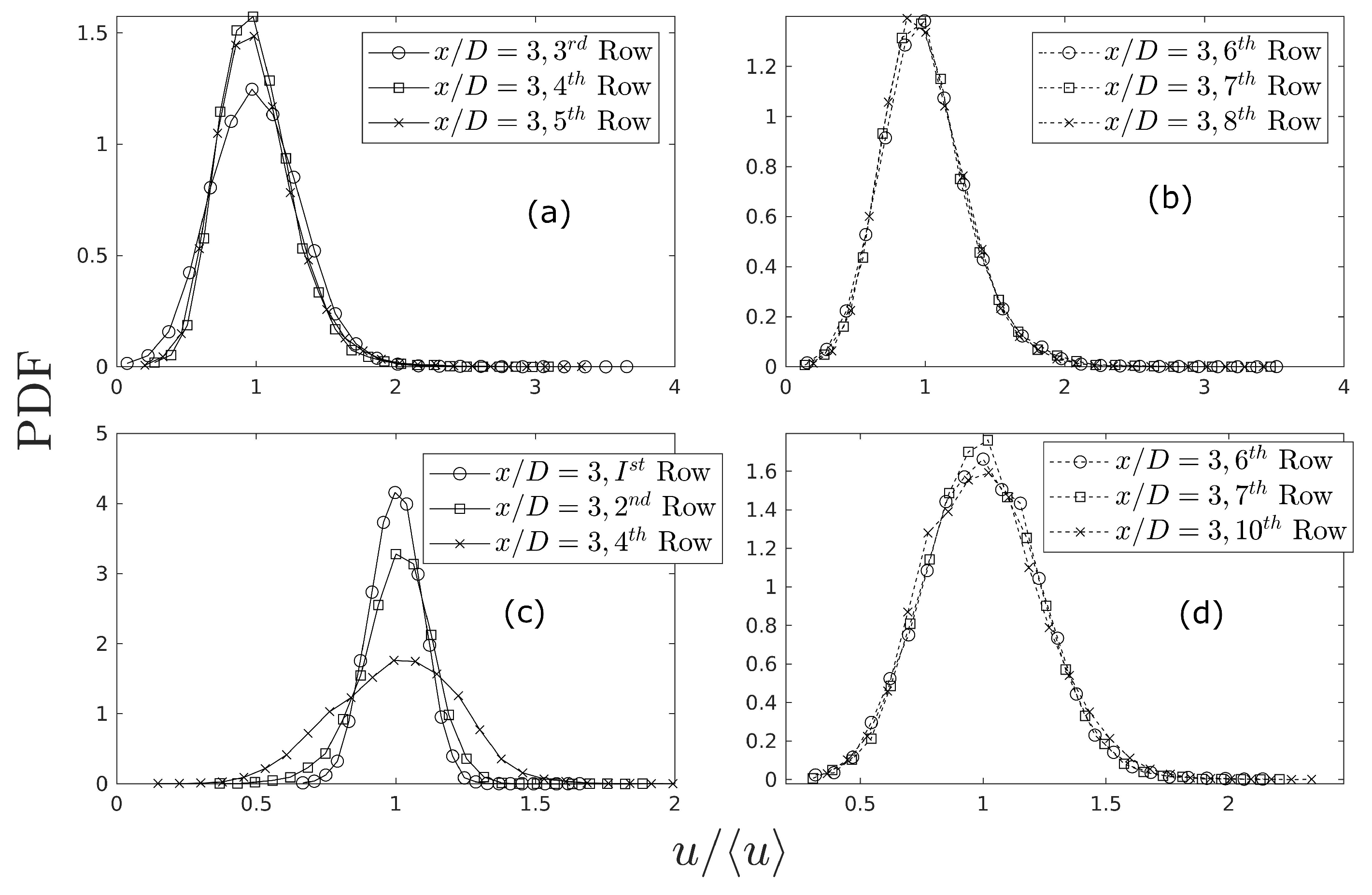
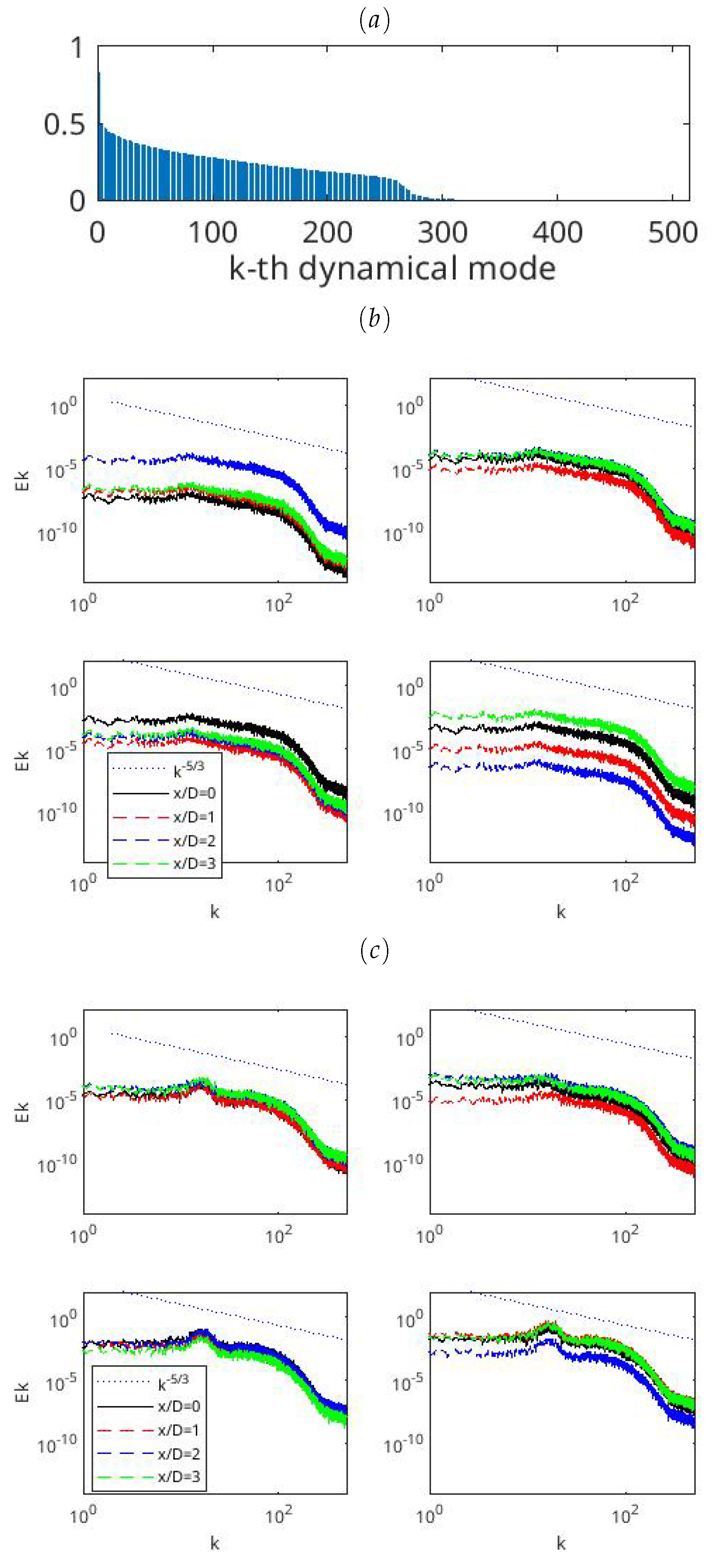
4.3. Time-Frequency Analysis of Wind Power Fluctuations in Wind Turbine Wakes

The Fourier transform of wind power fluctuations for individual turbines were reported to follow the power-law spectrum $k^{-5/3}$ in the wave number (k or in the corresponding frequency) domain [10,59]. This approach is inappropriate for non-stationary wind signals because shedding of coherent vorticity structures can produce amplitude and/or frequency modulations in the wind signals, e.g., at the center of wind turbine rotor. One method for capturing the envelope of the amplitude’s time variation is the Hilbert transform, where the instantaneous frequency represents the spectral characteristics. Alternatively, the wavelet transform is a technique that can directly characterize the time variation of all spectral components within a given frequency range, which instantaneously contributes to wind power fluctuations. Another dominant approach for the time-frequency analysis of turbulent flows is to either capture the spatial modes by the POD method or the dynamic modes by the DMD method.

Spectral Component Extraction by the POD Method

The POD method applies a modal decomposition of $u(\mathit{x},t)$ over an orthonormal basis ${\left\{{\varphi }_j\right\}}_{j=1}^r$,

$$u(\mathit{x},t)=\sum _{j=1}^r{c}_j\left(t\right){\varphi }_j\left(\mathit{x}\right).$$

(11)

Here, the orthonormality of the basis is such that $\langle {\varphi }_i,{\varphi }_j\rangle ={\delta }_{ij}$. Decomposition (11) is said to be complete if it converges to $u(\mathit{x},t)\in L^2\left(\mathsf{\Omega }\right)$ for all $(\mathit{x},t)\in \mathsf{\Omega }\times [0,T]$. Some texts refer to this decomposition as a generalized Fourier series if function $u(\mathit{x},t)$ satisfies periodic boundary conditions. The Bessel’s inequality and the Parseval’s equality, respectively,

$$\sum _{j=1}^{\infty }{c}_j^2\left|\right|{\varphi }_j{\left|\right|}^2\le {\left|\right|u\left|\right|}^2{\mathrm{and}\left|\right|u\left|\right|}^2=\sum _{j=1}^{\infty }{c}_j^2\left|\right|{\varphi }_j{\left|\right|}^2$$

(12)

guarantee that a finite number of coefficients $c_j=\langle u,{\varphi }_j\rangle /\left|\right|{\varphi }_j{\left|\right|}^2$ is sufficient for the best approximation of all $u(\mathit{x},t)$.

It is useful to introduce another orthonormal basis ${\left\{{\psi }_j\right\}}_{j=1}^{\infty }$ to characterize the time dynamics, which leads to $\langle c_i,c_j\rangle ={\sigma }_i^2$. Thus, Equation (11) takes the following form:

$$u(\mathit{x},t)=\sum _{j=1}^r\underset{c_j\left(t\right)}{\underbrace{{\psi }_j\left(t\right){\sigma }_j}}{\varphi }_j\left(\mathit{x}\right).$$

(13)

Unlike the wavelet- or the Fourier-based decompositions, the POD modes ${\varphi }_j$ lead to a data-driven spectral analysis, where the best-r POD modes capture the most energetic spectral components. Readers may follow Dai et al. [37] regarding the reconstruction of wind turbine wakes with POD and DMD methods. In the following analysis, we consider a set of n discrete-time velocity signals stored in matrix $\mathcal{U}\in {\mathbb{R}}^{n\times m}$. To implement the POD method, Equation (11), the singular value decomposition is applied, which provides an eigen decomposition of the (wind measurement) matrix $\mathcal{U}$ solving the following optimization problem:

$$\underset{\forall k,c_k\left(t\right)}{max}\left[{\displaystyle \frac{1}{n}}\sum _{d=1}^n{\langle c_k\left(t\right),u^{\prime }({\mathit{x}}_d,t)\rangle }^2\right]\mathrm{s}.\mathrm{t}.\langle c_i,c_j\rangle ={\sigma }_i^2{\delta }_{ij}.$$

The Fourier-based auto spectral density function (ASDF) $S_{uu}\left(f\right)$ captures the energy of a velocity signal $u({\mathit{x}}_d,t)$ as a function of frequency f and forms a Fourier transform pair with the autocorrelation of a velocity signal $u({\mathit{x}}_d,t)$ [60]. Parseval’s theorem states that

$$S_{uu}\left(f\right):={\int }_{-\infty }^{\infty }|u({\mathit{x}}_d,t){|}^{2}dt={\int }_{-\infty }^{\infty }{\left|\widehat{u}\left(f\right)\right|}^{2}df,\mathrm{where}\widehat{u}\left(f\right)={\int }_{-\infty }^{\infty }{e}^{-i2\pi ft}u({\mathit{x}}_d,t).$$

If most of the energy is contained in a few of the Fourier modes, ASDF captures the range of such frequencies. The Fourier method provides only a time-invariant amplitude and frequency for each spectral component, which is highly accurate for stationary signals.

To illustrate the POD method for time-frequency analysis of wind turbine wakes, we consider LES data in wakes of an array of wind turbines. First, we consider LES of the atmospheric boundary layer flow without considering any wind turbines and collect n discrete-time velocity signals $\mathcal{U}\in {\mathbb{R}}^{3n\times m}$. Since spectrum $S_{uu}\left(f\right)$ represents the energy density of both the coherent and the random components of the flow, this article considers the POD method to extract the spectrum of the energetic POD modes. In the atmospheric surface layer, the wind speed variability (and much of the land-surface exchange of fluxes) is characterized by ejection (of low-momentum eddies upward) and sweep (of high-momentum eddies downwards). Here, we consider the POD method to understand the low-dimensional structure underlying the sweep and ejection events.

The eigen decomposition allows to extract a low-dimensional structure of wind turbine wakes discarding POD modes associated with low-energy background. In Equation (11), the first coefficient $c_1\left(t\right)$, corresponding to the first POD mode ${\varphi }_1\left(\mathit{x}\right)$, when sampled at discrete times, indicates the direction along which the temporal fluctuations of wakes are most prominent. Ensuring that the projection of $q^{\prime }(\mathit{x},t)$ along $c_j\left(t\right)$ remains uncorrelated with that along $c_i\left(t\right)$ satisfies the orthogonality condition $\langle c_i\left(t\right),c_j\left(t\right)\rangle ={\sigma }_i^2{\delta }_{ij}$, where ${\sigma }_i^2$ reflects the variability (or energy) of the ith mode.

Figure 12 displays selected velocity signals and energy spectra on the vertical mid-plane of the domain. For simplicity, we let $X_d=0$ denote the first row of the $10\times 3$ array of turbines. The plot on the top of Figure 12a shows the streamwise component of the inflow velocity at $X_d=-17$. The plots other than that on the top of Figure 12a represent velocity at four turbines located at $X_d=0$ (Row 1), $X_d=5$ (Row 2), $X_d=10$ (Row 3), and $X_d=15$ (Row 4). For the plot at the bottom of Figure 12a, we zoomed in the time window to show the pattern of local fluctuations. The plots indicate episodes of turbulent bursts passing through the rotor region.

Figure 12b compares the energy spectra in the wakes of the first four turbines in the vertical mid-plane. For each row, we considered velocity signals at the turbine and three additional hub height locations in the wake behind the turbine. It may be simpler to denote each turbine by $x/D=0$ and three corresponding wakes by $x/D=1$, $x/D=2$, and $x/D=3$. The spectra on the left of the top row represent the wake between Row 1 and Row 2. Here, we scaled frequency $f=\omega /2\pi {\mathrm{s}}^{-1}$ with the time scale of $96D/U$ to obtain $k=96D\omega /\left(2\pi U\right)$, where $U=2.22$ m/s is the mean velocity at the hub height of the inlet boundary and $96D$ is the length of the domain. In the region between Row 2 and Row 3 (i.e., top right of Figure 12b), the energy is peaked at a wavenumber approximately between 15 and 45. In other words, large scale fluctuations of aerodynamic power occurred in the range of the length scale between $2D$ and $6D$. In the region between Row 3 and Row 5 (bottom row of Figure 12b), the energy containing length scales in the range of approximately between $0.5D$ and $14D$ exhibit a power law spectrum of $k^{-5/3}$. These spectra also indicate that the LES method resolves large eddies of the size at the rotor diameter or larger than that.

Figure 13a shows the principal components of the POD modes of the velocity fluctuations ${\mathcal{U}}^{\prime }$. The strength of principal components estimates the turbulence kinetic energy resolved by the LES method. From Figure 13a, we observe that about 300 POD modes captured approximately all of the resolved energy. If we consider the strongest r POD modes ${\left\{{\varphi }_k\left(\mathit{x}\right)\right\}}_{k=1}^r$ based on coefficients $\left\{c_k\right\}$, then the POD method extracts the low-dimensional flow features, where ${\mathcal{U}}_r=\overline{\mathcal{U}}+{\mathcal{U}}_r^{\prime }$ is a rank-r modal approximation to our velocity signals $\mathcal{U}$. Figure 13a indicates that the lowest rank represents the POD mode of the strongest energy. To illustrate the low-dimensional POD representation of wakes, we reproduced the spectra shown in Figure 12b ${\mathcal{U}}_1$ and ${\mathcal{U}}_4$.

The spectra of reconstructed velocity ${\mathcal{U}}_1$ account for the length scales that contribute to a majority of the energetic motion. Figure 13b shows the velocity spectra of ${\mathcal{U}}_1$ in the wake of four turbines, which represent the strongest POD mode, i.e., $r=1$. In comparison to the spectra shown in Figure 12b, the strongest POD mode (in Figure 13b) identifies the inertial range of eddies relatively clearly. In Figure 13c, we show the corresponding spectra considering the strongest four POD modes, i.e., the spectra of the reconstructed velocity ${\mathcal{U}}_4$ in the wake of the first four turbines. The peak of the energy of these stronger POD modes at length scales between $14D$ and $15D$ is attributed to the sweep events, i.e., the process of energy entrainment by vertical mixing (e.g., see [1]). However, more quantitative analysis would be useful to understand how vertical mixing may have contributed to these peaks in the spectra.

Now, we consider a surrogate power signals, $P({\mathit{x}}_d,t)\approx (1/2)\rho C_t\mathcal{A}{u}^3({\mathit{x}}_d,t)$. The ASDF of $P({\mathit{x}}_d,t)$ provides the effects of local wind speed variability on the spectral distribution of wind power at location ${\mathit{x}}_d$. Considering the Reynolds decomposition $u({\mathit{x}}_d,t)=\overline{u}+u^{\prime }({\mathit{x}}_d,t)$, we have the mean wind power ${\overline{P}}_d\approx (1/2)\rho C_t\mathcal{A}{\overline{u}}^3$ at ${\mathit{x}}_d$. Substituting the Reynolds decomposition of the velocity into the expression for the surrogate power signal $P({\mathit{x}}_d,t)$, we have the following cubic polynomial [13,59]:

$$P({\mathit{x}}_d,t)={\displaystyle \frac{1}{2}}\rho C_t\mathcal{A}\left[{\overline{u}}^3+3{\overline{u}}^2{u}^{\prime }+3\overline{u}{\left(u^{\prime }\right)}^2+{\left(u^{\prime }\right)}^3\right].$$

(14)

Neglecting the higher-order fluctuations, the following represents the linear relationship between power and velocity fluctuations,

$$P^{\prime }({\mathit{x}}_d,t)\approx {\displaystyle \frac{3}{2}}\rho C_t\mathcal{A}{\overline{u}}^2{u}^{\prime }\left(t\right).$$

(15)

In Equation (14), all of the higher order terms may be retained so that instead of Equation (15), we consider the following form of the wind power fluctuation:

$$P^{\prime }({\mathit{x}}_d,t)=P({\mathit{x}}_d,t)-{\overline{P}}_d.$$

(16)

Using the ASDF of the power fluctuations given by Equation (16), we can visualize the spectral distribution of wake interactions. Similar to the rank-r POD approximation of velocity, we considered the rank-r POD approximation of the power fluctuations $P_r^{\prime }({\mathit{x}}_d,t)$. The the ASDFs of the low-dimensional projection of power signals $P_1^{\prime }({\mathit{x}}_d,t)$ and $P_4^{\prime }({\mathit{x}}_d,t)$ are shown in Figure 14a,b. The spectra of fluctuating wind power (Figure 14) are similar to that of instantaneous winds. Interpretation of these plots follows that of the plots in Figure 13 (in the context of the present intention of vertical energy transport).

It is worth mentioning that POD is the dominant method for generating bases in reduced-order modeling of fluid flows. However, a major limitation of this approach is its empirical nature [61]. The basis functions produced by POD are tailored to represent the specific flow data used for their generation, but their accuracy may be lost when applied to conditions outside of the design space. Consequently, the reduced-order model may suffer a loss in accuracy when subjected to variations in flow parameters, such as Reynolds number, initial or boundary conditions, or external forcing.

5. Conclusions and Further Research Directions

For many years, vorticies have been used to model and simulate fluid flows. This article considers the vortex stretching mechanism as a scale-adaptive LES of wind farms. The concept draws from a well-established mathematical result in turbulence theory, which posits that the smoothness, regularity, and potential finite-time blow-up of Navier–Stokes solutions are linked to whether enstrophy production due to vortex stretching remains bounded over time and across all flow conditions. We leveraged this mathematical conjecture to model the energy flux cascade from large to small scales while incorporating the cumulative effects of land–atmosphere momentum exchanges on wind turbines.

To illustrate the scale-adaptive LES methodology for wind engineering applications, we considered two studies. In the first study, we compared the LES results of wind turbine wake profiles with wind tunnel measurements of the same. The results introduced new aspects of the dynamics underlying wind turbines and turbulence. In the second study, we considered the POD method to investigate the contribution of the most energetic large eddies in the wake recovery. The results indicated that the range of the strongest large eddies overlaps a relatively wider portion of the inertial range of turbulence. While turbines extracted the kinetic energy from all eddies, the spectra of the strongest POD modes hint at energy reaching in the vertical direction. This comment is consistent with the findings of Tian et al. [57] and Liu and Stevens [4]. We observed that a Gaussian kernel distributes the action of wind turbines across the actuator disk and the resulting actuator disk model captures the wind turbine wakes without needing the fully captured tip vorticies. The accuracy of such an LES prediction of wakes was confirmed by comparing the numerical results with the corresponding wind tunnel measurements. Further analysis of Reynolds stresses and dispersive stresses revealed that the proposed LES method performs equivalently to wind tunnel experiments for the test cases. Considering the probability density of instantaneously resolved velocity, we also observed that the LES method accurately predicts crucial points in the interaction of atmospheric boundary layer with wind farms.

A POD analysis of the available power from wind turbines and their wakes was presented. In particular, we considered velocity spectra to represent the turbulence transport of energy toward wake recovery. This approach allowed us to interpret the interaction between the wind turbines and the near-surface turbulence of the atmospheric boundary layer flow. The POD method also showed peak in the spectrum of wakes similar to the observed peaks in a wind farm.

We proposed for vortex stretching to be used not just to simulate wind farm atmospheric boundary layer, but also to analyze the flow structures in wind farms where multiple wakes interact with the atmospheric boundary layer. Johnson [20] and Hossen et al. [22] conducted similar analysis for isotropic flow leaving room for further analysis for turbulent flow over the built terrain. The approach considered in the present work to analytically filter the resolved flow also has the potential to directly enter into modeling subgrid-scale turbulence. We propose that wavelet-based filtering be directly applied to formulate scale-adaptive LES methodology. The work of the present study thus outlines new directions in fields of computational fluid dynamics and computational wind engineering.

References

1. Calaf, M.; Meneveau, C.; Meyers, J. Large eddy simulation study of fully developed wind-turbine array boundary layers. Phys. Fluids 2010, 22, 015110. [Google Scholar] [CrossRef]
2. Churchfield, M.J.; Lee, S.; Michalakes, J.; Moriarty, P.J. A numerical study of the effects of atmospheric and wake turbulence on wind turbine dynamics. J. Turbul. 2012, 13, N14. [Google Scholar] [CrossRef]
3. Doubrawa, P.; Quon, E.W.; Martinez-Tossas, L.A.; Shaler, K.; Debnath, M.; Hamilton, N.; Herges, T.G.; Maniaci, D.; Kelley, C.L.; Hsieh, A.S.; et al. Multimodel validation of single wakes in neutral and stratified atmospheric conditions. Wind Energy 2020, 23, 2027–2055. [Google Scholar] [CrossRef]
4. Liu, L.; Stevens, R.J. Effects of atmospheric stability on the performance of a wind turbine located behind a three-dimensional hill. Renew. Energy 2021, 175, 926–935. [Google Scholar] [CrossRef]
5. Stevens, R.J.; Meneveau, C. Flow structure and turbulence in wind farms. Annu. Rev. Fluid Mech. 2017, 49, 311–339. [Google Scholar] [CrossRef]
6. Asmuth, H.; Diaz, G.P.N.; Madsen, H.A.; Branlard, E.; Forsting, A.R.M.; Nilsson, K.; Jonkman, J.; Ivanell, S. Wind turbine response in waked inflow: A modelling benchmark against full-scale measurements. Renew. Energy 2022, 191, 868–887. [Google Scholar] [CrossRef]
7. Xie, S.; Archer, C.L. A numerical study of wind-turbine wakes for three atmospheric stability conditions. Bound. Layer Meteorol. 2017, 165, 87–112. [Google Scholar] [CrossRef]
8. Archer, C.L.; Vasel-Be-Hagh, A.; Yan, C.; Wu, S.; Pan, Y.; Brodie, J.F.; Maguire, A.E. Review and evaluation of wake loss models for wind energy applications. Appl. Energy 2018, 226, 1187–1207. [Google Scholar] [CrossRef]
9. Roy, S.B. Simulating impacts of wind farms on local hydrometeorology. J. Wind. Eng. Ind. Aerodyn. 2011, 99, 491–498. [Google Scholar]
10. Bossuyt, J.; Meneveau, C.; Meyers, J. Wind farm power fluctuations and spatial sampling of turbulent boundary layers. J. Fluid Mech. 2017, 823, 329–344. [Google Scholar] [CrossRef]
11. Wang, Q.; Luo, K.; Yuan, R.; Wang, S.; Fan, J.; Cen, K. A multiscale numerical framework coupled with control strategies for simulating a wind farm in complex terrain. Energy 2020, 203, 117913. [Google Scholar] [CrossRef]
12. Carbone, M.; Bragg, A.D. Is vortex stretching the main cause of the turbulent energy cascade? J. Fluid Mech. 2020, 883, R2. [Google Scholar] [CrossRef]
13. Alam, J. Interaction of vortex stretching with wind power fluctuations. Phys. Fluids 2022, 34, 075132. [Google Scholar] [CrossRef]
14. Batchelor, G.K. An Introduction to Fluid Dynamics; Cambridge University Press: Cambridge, UK, 2000. [Google Scholar]
15. Kundu, P.K.; Cohen, I.M.; Dowling, D.R.; Capecelatro, J. Fluid Mechanics; Elsevier: Amsterdam, The Netherlands, 2024. [Google Scholar]
16. Stevens, R.J. Dependence of optimal wind turbine spacing on wind farm length. Wind Energy 2016, 19, 651–663. [Google Scholar] [CrossRef]
17. Politis, E.S.; Prospathopoulos, J.; Cabezon, D.; Hansen, K.S.; Chaviaropoulos, P.; Barthelmie, R.J. Modeling wake effects in large wind farms in complex terrain: The problem, the methods and the issues. Wind Energy 2012, 15, 161–182. [Google Scholar] [CrossRef]
18. Abkar, M.; Porté-Agel, F. Influence of the Coriolis force on the structure and evolution of wind turbine wakes. Phys. Rev. Fluids 2016, 1, 063701. [Google Scholar] [CrossRef]
19. Van der Laan, M.P.; Sørensen, N.N. Why the Coriolis force turns a wind farm wake clockwise in the Northern Hemisphere. Wind. Energy Sci. 2017, 2, 285–294. [Google Scholar] [CrossRef]
20. Johnson, P.L. Energy Transfer from Large to Small Scales in Turbulence by Multiscale Nonlinear Strain and Vorticity Interactions. Phys. Rev. Lett. 2020, 124, 104501. [Google Scholar] [CrossRef]
21. Davidson, P.A. Turbulence: An Introduction for Scientists and Engineers; Oxford University Press: Oxford, UK, 2015. [Google Scholar]
22. Hossen, M.K.; Mulayath-Variyath, A.; Alam, J. Statistical Analysis of Dynamic Subgrid Modeling Approaches in Large Eddy Simulation. Aerospace 2021, 8, 375. [Google Scholar] [CrossRef]
23. Chamorro, L.P.; Porté-Agel, F. Effects of thermal stability and incoming boundary-layer flow characteristics on wind-turbine wakes: A wind-tunnel study. Bound. Layer Meteorol. 2010, 136, 515–533. [Google Scholar] [CrossRef]
24. Stevens, R.J.; Martínez-Tossas, L.A.; Meneveau, C. Comparison of wind farm large eddy simulations using actuator disk and actuator line models with wind tunnel experiments. Renew. Energy 2018, 116, 470–478. [Google Scholar] [CrossRef]
25. Porté-Agel, F.; Wu, Y.T.; Lu, H.; Conzemius, R.J. Large-eddy simulation of atmospheric boundary layer flow through wind turbines and wind farms. J. Wind. Eng. Ind. Aerodyn. 2011, 99, 154–168. [Google Scholar] [CrossRef]
26. Moser, R.D.; Haering, S.W.; Yalla, G.R. Statistical Properties of Subgrid-Scale Turbulence Models. Annu. Rev. Fluid Mech. 2021, 53, 255–286. [Google Scholar] [CrossRef]
27. Bose, S.T.; Park, G.I. Wall-modeled large-eddy simulation for complex turbulent flows. Annu. Rev. Fluid Mech. 2018, 50, 535–561. [Google Scholar] [CrossRef] [PubMed]
28. Mehta, D.; Van Zuijlen, A.; Koren, B.; Holierhoek, J.; Bijl, H. Large Eddy Simulation of wind farm aerodynamics: A review. J. Wind. Eng. Ind. Aerodyn. 2014, 133, 1–17. [Google Scholar] [CrossRef]
29. Sarlak, H.; Meneveau, C.; Sørensen, J.N. Role of subgrid-scale modeling in large eddy simulation of wind turbine wake interactions. Renew. Energy 2015, 77, 386–399. [Google Scholar] [CrossRef]
30. Smagorinsky, J. General circulation experiments with the primitive equations: I. The basic experiment. Mon. Weather Rev. 1963, 91, 99–164. [Google Scholar] [CrossRef]
31. Germano, M.; Piomelli, U.; Moin, P.; Cabot, W.H. A dynamic subgrid-scale eddy viscosity model. Phys. Fluids Fluid Dyn. 1991, 3, 1760–1765. [Google Scholar] [CrossRef]
32. Zang, Y.; Street, R.L.; Koseff, J.R. A dynamic mixed subgrid-scale model and its application to turbulent recirculating flows. Phys. Fluids A Fluid Dyn. 1993, 5, 3186–3196. [Google Scholar] [CrossRef]
33. Kelley, N.D.; Jonkman, B.J.; Scott, G.; Bialasiewicz, J.; Redmond, L.S. Impact of Coherent Turbulence on Wind Turbine Aeroelastic Response and Its Simulation; Technical Report; National Renewable Energy Lab (NREL): Golden, CO, USA, 2005. [Google Scholar]
34. Chamorro, L.; Hill, C.; Neary, V.; Gunawan, B.; Arndt, R.; Sotiropoulos, F. Effects of energetic coherent motions on the power and wake of an axial-flow turbine. Phys. Fluids 2015, 27, 055104. [Google Scholar] [CrossRef]
35. Taylor, G.I. Production and dissipation of vorticity in a turbulent fluid. Proc. R. Soc. Lond. Ser. A Math. Phys. Sci. 1938, 164, 15–23. [Google Scholar]
36. Alam, J.M.; Fitzpatrick, L.P. Large eddy simulation of flow through a periodic array of urban-like obstacles using a canopy stress method. Comput. Fluids 2018, 171, 65–78. [Google Scholar] [CrossRef]
37. Dai, X.; Xu, D.; Zhang, M.; Stevens, R.J. A three-dimensional dynamic mode decomposition analysis of wind farm flow aerodynamics. Renew. Energy 2022, 191, 608–624. [Google Scholar] [CrossRef]
38. Wyngaard, J.C. Toward numerical modeling in the “Terra Incognita”. J. Atmos. Sci. 2004, 61, 1816–1826. [Google Scholar] [CrossRef]
39. Deardorff, J.W. Numerical investigation of neutral and unstable planetary boundary layers. J. Atmos. Sci. 1972, 29, 91–115. [Google Scholar] [CrossRef]
40. Borue, V.; Orszag, S.A. Local energy flux and subgrid-scale statistics in three-dimensional turbulence. J. Fluid Mech. 1998, 366, 1–31. [Google Scholar] [CrossRef]
41. Singh, J.; Alam, J. Impact of atmospheric turbulence on wind farms sited over complex terrain. Phys. Fluids 2024, 36, 095170. [Google Scholar] [CrossRef]
42. Singh, J.; Alam, J. Dynamic modelling of near-surface turbulence in large eddy simulation of wind farms. arXiv 2022, arXiv:2205.00352. [Google Scholar]
43. Singh, J.; Alam, J.M. Large-Eddy Simulation of Utility-Scale Wind Farm Sited over Complex Terrain. Energies 2023, 16, 5941. [Google Scholar] [CrossRef]
44. Martínez-Tossas, L.A.; Churchfield, M.J.; Leonardi, S. Large eddy simulations of the flow past wind turbines: Actuator line and disk modeling. Wind Energy 2015, 18, 1047–1060. [Google Scholar] [CrossRef]
45. Wu, C.; Wang, Q.; Yuan, R.; Luo, K.; Fan, J. Large eddy simulation of the layout effects on wind farm performance coupling with wind turbine control strategies. J. Energy Resour. Technol. 2022, 144, 051304. [Google Scholar] [CrossRef]
46. Hossain, M.A.; Alam, J.M. Assessment of a symmetry-preserving JFNK method for atmospheric convection. Comput. Phys. Commun. 2021, 269, 108113. [Google Scholar] [CrossRef]
47. Johnson, P.L. On the role of vorticity stretching and strain self-amplification in the turbulence energy cascade. J. Fluid Mech. 2021, 922, A3. [Google Scholar] [CrossRef]
48. Sarlak, H.; Pierella, F.; Mikkelsen, R.; Sørensen, J.N. Comparison of two LES codes for wind turbine wake studies. IOP J. Phys. Conf. Ser. 2014, 524, 012145. [Google Scholar] [CrossRef]
49. Martinez-Tossas, L.A.; Churchfield, M.J.; Yilmaz, A.E.; Sarlak, H.; Johnson, P.L.; Sørensen, J.N.; Meyers, J.; Meneveau, C. Comparison of four large-eddy simulation research codes and effects of model coefficient and inflow turbulence in actuator-line-based wind turbine modeling. J. Renew. Sustain. Energy 2018, 10, 033301. [Google Scholar] [CrossRef]
50. Chamorro, L.P.; Porte-Agel, F. Turbulent flow inside and above a wind farm: A wind-tunnel study. Energies 2011, 4, 1916–1936. [Google Scholar] [CrossRef]
51. Réthoré, P.E.; van der Laan, P.; Troldborg, N.; Zahle, F.; Sørensen, N.N. Verification and validation of an actuator disc model. Wind Energy 2014, 17, 919–937. [Google Scholar] [CrossRef]
52. Jimenez, A.; Crespo, A.; Migoya, E.; García, J. Advances in large-eddy simulation of a wind turbine wake. IOP J. Phys. Conf. Ser. 2007, 75, 012041. [Google Scholar] [CrossRef]
53. Wu, Y.T.; Porté-Agel, F. Large-eddy simulation of wind-turbine wakes: Evaluation of turbine parametrisations. Bound. Layer Meteorol. 2011, 138, 345–366. [Google Scholar] [CrossRef]
54. Wu, Y.T.; Porté-Agel, F. Simulation of turbulent flow inside and above wind farms: Model validation and layout effects. Bound. Layer Meteorol. 2013, 146, 181–205. [Google Scholar] [CrossRef]
55. Yang, D.; Meneveau, C.; Shen, L. Dynamic modelling of sea-surface roughness for large-eddy simulation of wind over ocean wavefield. J. Fluid Mech. 2013, 726, 62–99. [Google Scholar] [CrossRef]
56. Yang, D.; Meneveau, C.; Shen, L. Large-eddy simulation of offshore wind farm. Phys. Fluids 2014, 26, 025101. [Google Scholar] [CrossRef]
57. Tian, W.; Ozbay, A.; Yuan, W.; Sarakar, P.; Hu, H.; Yuan, W. An experimental study on the performances of wind turbines over complex terrain. In Proceedings of the 51st AIAA Aerospace Sciences Meeting including the New Horizons Forum and Aerospace Exposition, Grapevine, TX, USA, 7–10 January 2013; pp. 7–10. [Google Scholar]
58. Poggi, D.; Katul, G.; Albertson, J. A note on the contribution of dispersive fluxes to momentum transfer within canopies. Bound. Layer Meteorol. 2004, 111, 615–621. [Google Scholar] [CrossRef]
59. Bandi, M.M. Spectrum of wind power fluctuations. Phys. Rev. Lett. 2017, 118, 028301. [Google Scholar] [CrossRef]
60. Pope, S.B. Turbulent Flows; IOP Publishing: Bristol, UK, 2001. [Google Scholar]
61. Hay, A.; Borggaard, J.T.; Pelletier, D. Local improvements to reduced-order models using sensitivity analysis of the proper orthogonal decomposition. J. Fluid Mech. 2009, 629, 41–72. [Google Scholar] [CrossRef]
Figure 1. (a) The computational domain L x × L y × L z = [ 5.4 × 0.9 × 0.45 ] m3 for LES of an isolated turbine. (b) The layout of an array of 10 × 3 wind turbines in the computational domain L x × L y × L z = [ 14.4 × 1.8 × 0.675 ] m3. Only the first four rows of the array 10 × 3 are shown for clarity. The streamwise and spanwise spacing between wind turbines are S x = 5 D and S y = 4 D , respectively.
Wind 04 00015 g001
Figure 2. Isosurface plots of the vorticity magnitude | ω | for 10 × 3 array of wind turbines.
Wind 04 00015 g002
Figure 3. Vertical profiles of mean streamwise velocity using the G-ADM simulated with five meshes (see Table 1 for the resolutions of cases M1–M5). The velocity was sampled on 8 lines in the vertical mid-plane of the domain. The locations of these lines are at x / D = 1 , x / D = 2 , x / D = 3 , x / D = 5 , x / D = 7 , x / D = 10 , x / D = 14 , and x / D = 20 , where x / D = 0 denotes the location of the turbine.
Wind 04 00015 g003
Figure 4. A comparison of vertical profiles of mean streamwise velocity among wind tunnel data [23], corresponding LES data (ALM and ALM + structure) of [24], and present LES results (M5) in the case of a standalone wind turbine.
Wind 04 00015 g004
Figure 5. A comparison of vertical profiles of mean streamwise velocity in the vertical mid-plane of the domain. The symbol ∘ refers to wind-tunnel measurements [23], solid orange and yellow lines represent ALM and ALM + structure, respectively, referencing LES data [24], whereas purple line represents the present LES results using G-ADM model (WF2). Each row of plots corresponds to the wake of a row of the wind farm, such as x / D = 1 , x / D = 2 , x / D = 3 , x / D = 4 .
Wind 04 00015 g005
Figure 6. (a) Incoming vertical profile of the stream-wise velocity normalized with its hub-height value; (b) vertical profiles of the streamwise velocity u ¯ ( z ) in the wake at x / D = 2 for the mid-column of the 10 × 3 array for Rows 5–6; and (c) vertical profiles of the streamwise velocity deficit, i.e., the difference of the data in (a) from that in (b).
Wind 04 00015 g006
Figure 7. A comparison of the mean streamwise velocity at top tip, hub-height, and bottom tip. The data correspond to velocity at four stream-wise locations: x / D = 1 , x / D = 2 , x / D = 3 , and x / D = 4 across the central column and relative to each of the first seven rows of the wind turbine array.
Wind 04 00015 g007
Figure 8. (a) Vertical profiles of the turbulence intensity ( σ / U h u b denoting σ = τ 11 R ) obtained by experiment [23], reference LES data [24], and G-ADM (case M5, see Table 1) of present LES. (b) Vertical profiles of the kinematic shear stress ( u w ˜ ) obtained by experiment [23], reference LES [53], and G-ADM (M5) of present LES.
Wind 04 00015 g008
Figure 9. Vertical profiles of horizontally averaged (a) kinetic energy (k) (b) Reynolds shear stress ( τ 13 R ) and dispersive shear stress ( τ 13 D ). The vertical profiles are normalized by the streamwise velocity, U h u b 2 .
Wind 04 00015 g009
Figure 10. The top panel shows the probability density function (PDF) of instantaneously resolved velocity u ¯ ( x , t ) in Region-I ( z / D < 1.34 ). In contrast, the bottom panel shows the PDF of Region-II ( z / D > 1.34 ) in a wind farm. Subfigure (a) shows Region-I for the 3rd, 4th, and 5th rows; subfigure (b) shows Region-I for the 6th, 7th, and 8th rows. Subfigure (c) shows Region-II for the 1st, 2nd, and 4th rows; subfigure (d) shows Region-II for the 6th, 7th, and 10th rows.
Wind 04 00015 g010
Figure 11. Sensitivity of model constant c k . The figure shows turbulence stresses for three different model coefficients c k in the case of scale-adaptive LES coupled with the wind turbine model G-ADM at various streamwise locations: x / D = 2 , x / D = 3 , x / D = 5 , x / D = 7 , and x / D = 10 . The subplots depict: (a) the streamwise component of Reynolds stress u u ˜ , (b) the spanwise component v v ˜ , (c) the vertical or surface-normal component w w ˜ , and (d) the shear stress u w ˜ .
Wind 04 00015 g011
Figure 12. (a) Streamwise Component of the instantaneous velocity u ( x d , t ) in the vertical mid-plane at four hub height locations x d . These locations are (from top to bottom): at the inlet, at the first row of the wind turbine array ( x / D = 0 ), at x / D = 1 , and at x / D = 2 . (b) Energy spectra in the wakes of the first four turbines in the vertical mid-plane, compared at four locations in the wake: x / D = 0 , x / D = 1 , x / D = 2 , and x / D = 3 . The reference k 5 / 3 slope is also shown.
Wind 04 00015 g012
Figure 13. Energy distribution of rank—r flow structures in the wake of first 4 turbines in the vertical mid-plane of the domain. (a) Distribution of POD coefficients. Spectra for r = 1 (b) and r = 4 (c). The dashed line represents k 5 / 3 , where k = 96 f D / ( 2 π U ) .
Wind 04 00015 g013
Figure 14. The spectrum of wind power fluctuations reconstructed with POD modes. (a) Spectrum reconstructed with the most dominant POD mode, and (b) spectrum reconstructed with the first four POD modes. The spectra correspond to the first four turbines ( x / D = 0 ) in the vertical mid-plane of the domain and their wakes at x / D = 1 , x / D = 2 , and x / D = 3 . The dashed line represents k 5 / 3 , where k = 96 f D / U .
Wind 04 00015 g014