Uncertainty in the Calibration Transfer of Solar Irradiance Scale: From Absolute Cavity Radiometers to Standard Pyrheliometers

Abstract

In this work, the method for calculation of uncertainty of pyrheliometers’ responsivity during their outdoor calibration process in the laboratory is exposed. It is applied first for calibration of standard pyrheliometers by comparison to cavity radiometers, and after for calibration of an end-user pyrheliometer against that standard pyrheliometer. The dissemination of the WRR irradiance scale is illustrated in practice and the increasing uncertainty in the traceability chain is quantified. The way of getting traceability to both WRR scale and to SI units in the current situation, where the shift between these radiometric scales is pending to be solved, is also explained. However, the impact of this gap between scales seems to be more important for calibrations of reference Class A pyrheliometers than in the final determination of DNI irradiance, because in this case, the cumulative uncertainty is large enough as to not significantly be affected for the difference. The way to take into account different correction terms in the measurement model function, and how to compute the corresponding uncertainty, is explained too. The influence of temperature of some pyrheliometers during calibration process and the potential impact on the DNI irradiance calculated with these instruments is exemplified.

1. Introduction

Solar radiation is probably the most influential magnitude on Earth’s climate system and on its energetic balance. It is measured and studied in fields of science such as astronomy and space physics, medicine, agriculture, architecture, or climatology and meteorology. It is, of course, the primary energy source for solar thermal and photovoltaic (PV) conversion systems, and fundamental biological and climatic processes on Earth would not be possible without the thermal and/or lighting supply from the Sun.

The scientific community, in the framework of the Intergovernmental Panel on Climate Change (IPCC), is carrying out a huge effort to understand the mechanisms governing Earth’s climate, and are demanding a higher accuracy from the experimental data and from the climatic models [1]. In this sense, the Global Climate Observing System (GCOS) [2] considers the Earth Radiation Budget (ERB) and the Surface Radiation Budget (SRB) as some of the Essential Climate Variables (ECV) to be observed. ERB is obtained from measurements in space of the Total Solar Irradiance (TSI) received from the Sun and of the total irradiance (long- and short-wave) from the Earth’s surface, while SRB also requires on-ground measurements of solar irradiance.

GCOS also pointed out the importance of a continuous recording of solar radiation and posed basic requisites for its measurement: 1 W·m⁻² in absolute accuracy and 0.3 W·m⁻² per decade in stability [3]. For reference, last-accepted values of the Sun’s irradiance at the mean Earth–Sun distance (1 AU), the so-called solar constant, are ~1361 W m⁻² [4,5,6], so that figure-of-merit means obtaining accuracies better than 0.075% (≈1/1361) in TSI measurements (around ~0.1% at ground-level for 1000 W·m⁻²). Requisites suggested two decades ago for space radiometers by NIST were even more demanding: spectral radiation reflected from terrestrial surface to be measured with an accuracy of 0.2%, spectral solar irradiance and TSI up to 0.01% [7,8].

On the other hand, monitoring systems for photovoltaic and thermal solar plants are progressively requiring better capabilities and higher reliability for devices measuring solar irradiance, as suggested in the IEC 61724-1 standard [9]. This is due to the important economic consequences that a correct evaluation of energy production and performance ratio in PV solar plants has.

Obviously, adequate instrumentation is necessary to meet these requirements. The modern history of solar radiometry includes plenty of technical developments, instruments, and metrology scales, revealing an impressive dedication for its correct assessment with increasing accuracy, and the key importance of these measurements along decades. Reviews on the evolution of instruments and scales in solar radiometry can be found elsewhere [10,11,12,13,14,15,16,17,18].

Currently, instruments at the highest metrological level for measuring solar irradiance are the so-called Absolute Cavity Radiometers (ACR), which work under the Principle of Electrical Substitution or Compensation [19,20]. First ACR versions were developed in the JPL-NASA at the end of the 1960s [21,22] and were conceived for space measurements of TSI and ERB. Adaptations of these ACRs were readily applied for the on-ground measurement of irradiance and, thanks to their great accuracy and better performance when compared to Angström and Abbot’s silver disk radiometers, give rise to the definition in 1976 by the WMO of a new scale in solar irradiance (being currently into effect): the World Radiometric Reference (WRR) scale [23]. WRR was defined as the mean value of 15 selected cavity radiometers which took part in the IV International Pyrheliometer Comparison (IPC-IV, 1975), the World Standard Group (WSG). Despite WRR is based on an ‘artifact’ or ‘prototype’ (as in the past with the unit of mass, the kilogram), it is recognized by consensus as the primary reference of solar irradiance, and every radiometer in WSG is considered as the practical realization (mise en practique) of the W m⁻² unit.

Thus, during subsequent IPCs (every 5 years), WRR solar irradiance scale is disseminated, by comparison to WSG, to other cavity radiometers and pyrheliometers from WMO regional and national radiometric centers, National Metrology Institutes (NMI), R&D institutions, BSRN stations, and commercial companies from all around the world. Then, in a hierarchical sequence of calibration steps, the scale is transferred to secondary standard pyrheliometers and pyranometers, to working standards and to field sensors.

On the other hand, solar irradiance, despite its longer trajectory, is fully integrated into SI and under the scope of the International Committee for Weights and Measures (CIPM) only since 2008, being one of the youngest magnitudes in the SI. The quantities related to solar radiation that can potentially be claimed by an NMI in their Calibration and Measurement Capabilities (CMC) [24] are: (a) responsivity, solar, power; (b) responsivity, solar, irradiance; and (c) responsivity, solar, spectral, irradiance.

Correspondence between WRR scale and SI radiometric laboratory scale (based on absolute cryogenic radiometers) have periodically been checked [25,26,27,28,29]. In this way, traceability to WRR automatically provides traceability to SI units. A deviation of 0.3% was usually applied for accounting for the difference between scales [28]. Nevertheless, the status of the WRR scale is currently under review by WMO and CIPM, because of some deviations found in the last comparisons [10,29,30]. The shift between scales is temporarily solved by the application of a correction or transfer factor. Recent intercomparisons and tests with new instruments are showing that compatibility between WRR-SI scales could be solved soon [29,31,32].

However, many of these developments, motivations, and problems within solar irradiance metrology are ignored or overlooked when users perform routine daily measurements of solar irradiance in solar thermal and PV plants, weather stations, and other applications. Probably, the responsivity (or sensitivity or calibration factor) of a solar sensor is the key parameter for many end users, the only relevant one for them in order to correctly estimate the solar irradiance. The metrology level or class of a sensor is probably less important, except for the relationship with its cost. Uncertainty is in turn a term not well understood and integrated in these daily measurements.

Additionally, much more attention is given to pyranometers than to pyrheliometers in the literature, probably because these are more easily calibrated, and the magnitudes of influence in their operation are less, or their effects are not as important as for pyranometers, although they exist [33,34,35,36], and because pyranometers, as global hemispherical sensors, are used as reference sensors for other devices needing to know global (in plane or horizontal) solar irradiance values (e.g., PV solar modules and solar cells).

However, it is important to keep in mind that reference pyranometers are calibrated by means of reference standard pyrheliometers, by comparison either to cavity radiometers themselves or to secondary reference pyrheliometers, which have in turn been calibrated against cavity radiometers. Therefore, calibration and uncertainty of pyrheliometers are of great importance in the transmission of traceability of WRR solar irradiance scale, despite few papers being devoted to this subject.

In particular, the current into-effect edition of ISO 9059:1990 [37] does not cover the computation of the uncertainty associated to the calibration of a pyrheliometer, and ASTM G213–17 guide [38] mainly refers to pyranometers, while pyrheliometers are briefly referred to. The same occurs with references found in the literature, where pyrheliometers are treated to a much lower extent than pyranometers, or where pyrheliometer uncertainty is analyzed in an incomplete way, and sometimes with focus on the uncertainty of the DNI irradiance [39,40,41,42,43,44]. It is important to mention that ISO standards in the field of solar energy are being currently under revision, so it is a good moment to show and propose realistic methods of calibration and computation of uncertainty that serve for the development of these standards. On the other hand, the huge increase of installed power of solar PV and thermal plants that is being experienced in many countries, with the corresponding increase on the number of solar sensors and monitoring systems, makes the diffusion of test and calculation methods used by laboratories for calibrating these instruments, as well as the magnitudes of influence and how the values of uncertainty included in the calibration certificates are obtained, of great interest for PV installers, engineers, and plant managers, and can support financiers and developers in the deployment of these solar energy projects.

In short, this work is focused on describing the dissemination of the WRR solar irradiance scale from cavity radiometers to standard pyrheliometers, and from these to end-use instruments of lower metrological level, and how much the uncertainty increases at each successive calibration stage. It is also addressed to calculate the real figures of uncertainty for practical cases.

The main contributions of this work are the explicit treatment of uncertainty computation in every transference step along the WRR scale, with the measurement model functions of use in each one, on the basis of the calibration procedures developed in our laboratory according to ISO standards. While calibration procedures applied between standard pyrheliometers are more commonly considered in the literature, this paper also includes first, high-level calibration phases using cavity radiometers. The ways to account for different magnitudes of influence and how to evaluate their impact in terms of uncertainty are also described, with a degree of detail that is missed in other works. Important notes about to which instrument or to which magnitude a given term has to be attributed are introduced and justified. Despite the main content of the work being based on simple equations, a more general approach for including dependences on additional variables in the measurement function, at the cost of managing more complex equations, is also described (see Appendix A), which is also an original input of this work. Temperature and zero-irradiance voltage offsets, as examples of the type of dependences that can be considered following this general procedure, are explicitly described. As another important contribution, traceability to both WRR scale and to SI units is integrated into the computation, comparing the differences in uncertainty obtained in every case. The impact of this gap between scales is quantitatively evaluated at the different transference levels, and the reasons why it has a larger impact for calibrations of reference Class A pyrheliometers with cavity radiometers than in the final determination of DNI irradiance are explained. Procedures for dealing with instruments having noticeable dependences on temperature, both for calibration and for irradiance evaluation, are also suggested.

2. Methods

In this section, procedures and theoretical formulas for computation of the uncertainty in the calibration of pyrheliometers, following the WRR traceability chain, are derived. First, the traceability in the solar irradiance scale is briefly exposed. Afterward, operational equations for pyrheliometers, of general application, are posed. The experimental procedures for calibration and transfer of the irradiance scale from ACR to reference standard pyrheliometers, and from these to secondary devices, are also described. These correspond to the implementation in the PVLab-CIEMAT of the guidelines contained into ISO standards. Next, detailed derivation of the uncertainty components for every calibration procedure, and how the different contributions can be computed, are explained.

2.1. Traceability on the Solar Irradiance Scale

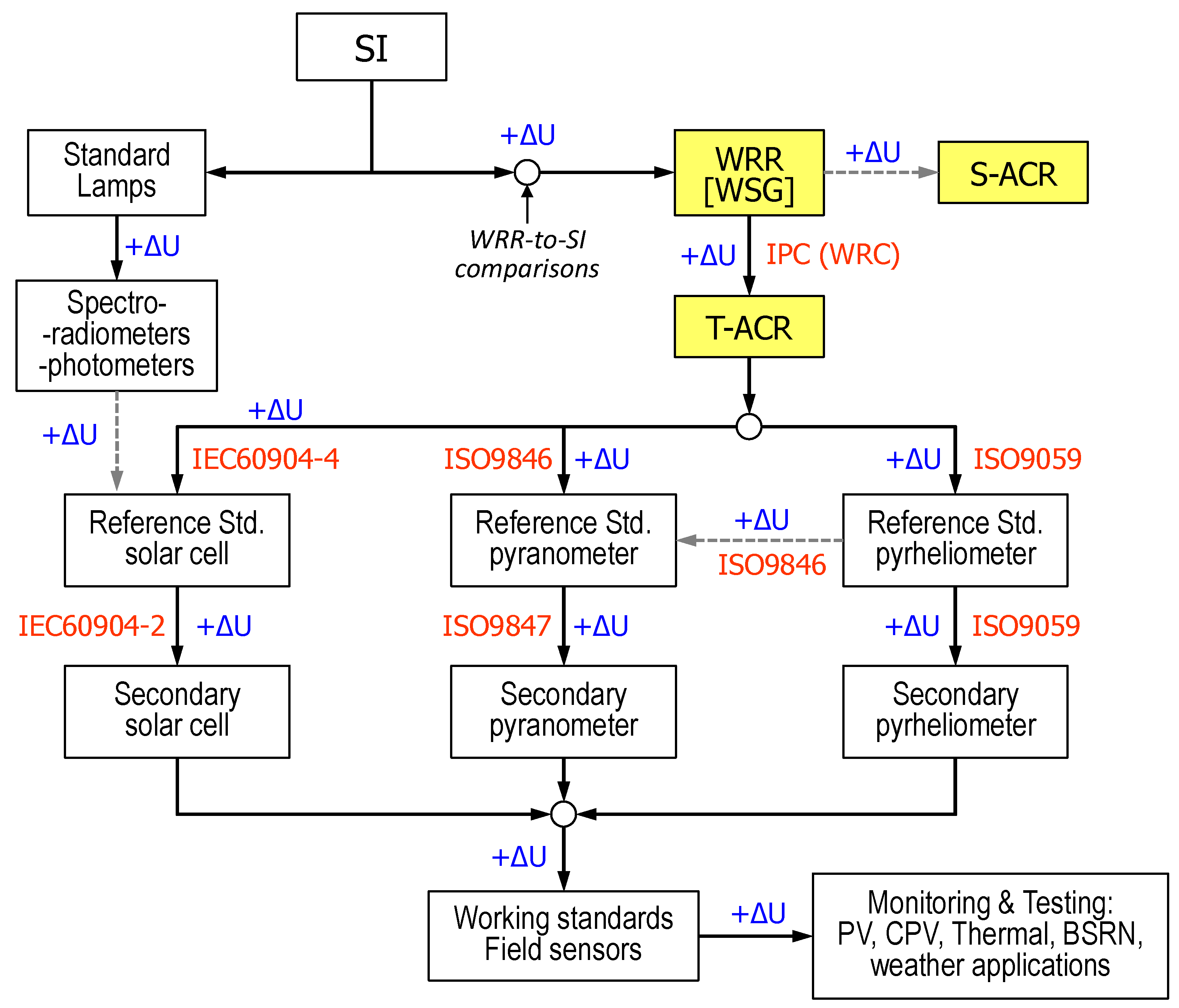
Figure 1 shows the scheme of hierarchical dissemination of WRR solar irradiance scale among instruments of different metrological level and the ISO standards of application on this field. In fact, WRR scale can be considered as a direct normal solar irradiance (DNI) scale that is extended or broadened to the measurement of global or hemispherical solar irradiance, and to other sensors operating under physical principles different from those of cavity radiometers. Core parts of these group of standards refer to traceability transfer by calibration between cavity radiometers and pyrheliometers (ISO 9059:1990 [37]), between cavity radiometers and pyranometers (ISO 9846:1993 [45]), and between cavity radiometers and PV solar cells (IEC 60904-4:2019 [46]). The diagram also considers the transfer between pyranometers (ISO 9847:1992 [47]), between pyrheliometers (the same ISO 9059:1990) and between PV solar cells (IEC 60904-2:2015 [48]). Moreover, these same standards allow the successive transfer and dissemination of the scale to working standards and field sensors. Finally, another fundamental standard is ISO 9060:2018 [49] which stablishes a classification for pyranometers and pyrheliometers according to their accuracy and metrological level, and estates the technical requirements for getting a given class for every sensor. PVLab-CIEMAT carry out calibrations of pyranometers, pyrheliometers, and solar cells in a systematic way by the implementation of internal procedures according to these standards.

There also exist standards developed by ASTM equivalent to these ISO ones. For example, to mention some of them, the ASTM E816-15 standard [50] is equivalent to ISO 9059, the ASTM E824-10 [51] and G207-11 [52] standards are harmonized to ISO 9847, and ASTM G167-00 [53] to ISO 9846.

Finally, it is important to include in this description the WMO CIMO guide [54], in which chapter 7 is devoted to instruments for measuring of solar radiation, their classification, and their methods of calibration.

2.2. Pyrheliometer Responsivity and Measurement Equations

In general, an ideal pyrheliometer is a solar radiation sensing instrument whose electrical output signal is linearly proportional to the incoming DNI irradiance within a narrow solid angle (around ~5°). This solid angle allows the pyrheliometer to receive solar radiation from the solar disk itself and also from the circumsolar or aureole region. There are different types of pyrheliometers available on the market, which can roughly be classified as:

• Passive-type pyrheliometers, e.g., with an analog voltage or current signal directly generated with a simple sensor (e.g., a thermopile, a photoelectric, or a pyroelectric sensor). Classic thermopile-based ones usually give output voltages of the order of [0 → 10] mV or [0 → 20] mV;
• Active-type pyrheliometers, with the addition of electric/electronic circuitry adapting the signal produced by those single sensors (e.g., outputs in the form of current loops, voltage amplified signals, temperature-drift compensation circuits, etc.). An example of nominal outputs from active-type devices can be, e.g., within [0 → 1] V, [0.1 → 1] V, [4 → 20] mA ranges for irradiances between 0 to 1600 W·m⁻².
• Smart or digital-type pyrheliometers are based on microprocessor circuits and embedded signal meters, which give a direct value of the irradiance (and other signals, such as temperature, raw voltages, etc.) through digital protocols (e.g., MODBUS, SPI, I²C). These digital instruments use internally stored constants (with reprogrammable values) for realizing this conversion.

In all these cases, the responsivity R of the pyrheliometer can be defined as the relationship between its electrical output signal and the solar DNI irradiance E producing such a signal:

$$R=\frac{V-V_0}{E}\hspace{1em}\mathrm{or}\hspace{1em}R=\frac{I-I_0}{E},$$

(1)

where V, I is the output signal of the pyrheliometer at a irradiance level E and V₀, I₀ is the output signal when irradiance is zero (called zero-irradiance signal). Thus, in SI, E is given in units of W·m⁻², and R is expressed in V·W⁻¹·m² or in A·W⁻¹·m². Sometimes, a calibration factor F (being F = 1/R) is used instead of the responsivity, as in ISO 9059:1990. In the case of digital pyrheliometers, the calibration factor would be, for example, the ratio of the measured irradiance by the pyrheliometer under test to the reference irradiance. However, even in these instruments, the responsivity could be calculated by using the raw output values from the sensor.

A couple of important details about Equation (1) have to be given:

• It does not make explicit any of the possible corrections, deviations, or dependences of responsivity, such as those due to zero-irradiance offsets (δV₀, δI₀), temperature (T), tilt angle (Z), spectral distribution (λ), etc. To keep the analysis simple in the main text, a more general method to include some of these additional corrections is considered in the Appendix A.
• V₀, I₀ values stand for the nominal zero-irradiance value of the pyrheliometers and not for the possible offsets δV₀, δI₀ of these zero-irradiance signals, which are considered as a correction or deviation parameter. Then, V₀, I₀ in Equation (1) are ideal, theoretical values, while δV₀, δI₀ are to be (experimentally, numerically) obtained. For example, I₀ = 4 mA for a current loop output pyrheliometer, and V₀ = 0 for a classic analog thermopile-type pyrheliometer.

Later, when the pyrheliometer is used for estimating DNI irradiance E in a particular application, its value is calculated as:

$$E=\frac{V-V_0}{R}\hspace{1em}\mathrm{or}\hspace{1em}E=\frac{I-I_0}{R},$$

(2)

This work is focused on the uncertainty of the calibration of pyrheliometer responsivity and not on the uncertainty of the DNI irradiance that is a posteriori calculated with the pyrheliometer through Equation (2), although the methodology here exposed can be extended for that purpose. Some details are discussed later in this regard.

It can be stated that the calibration of pyrheliometers is conceived in international standards on the basis of the application of Equation (1), even though the zero-irradiance signal could not explicitly be considered. When a (Class A) standard reference pyrheliometer is calibrated against a cavity radiometer, the value of DNI irradiance E is given by the cavity radiometer. This will be named Procedure A in this work. After, when a secondary or a field pyrheliometer is calibrated by comparison to a standard reference pyrheliometer (named Procedure B in this work), the value of E is obtained through the output values of the reference pyrheliometer and, thus, Equation (1) is modified as follows:

$$R_D=\frac{V_D-V_{D0}}{E}=\frac{V_D-V_{D0}}{V_R-V_{R0}}·R_R\hspace{1em}\mathrm{or}\hspace{1em}{R}_D=\frac{I_D-I_{D0}}{E}=\frac{I_D-I_{D0}}{V_R-V_{R0}}·R_R,$$

(3)

where V_D, V_D0 (I_D, I_D0) are the output signals of the pyrheliometer or device under test (DUT), V_R, V_R0 are the output signals of the reference (REF) pyrheliometer, and R_R is its calibrated responsivity.

In the particular case of a current loop output signal pyrheliometer, it can be measured directly (digital multimeter DMM used as an ammeter) through the voltage drop across the terminals of a shunt resistor of value R_SH (DMM used as a voltmeter), and therefore:

$$I_D-I_{D0}=\frac{1}{R_{SH}}·\left(V_D-V_{D0}\right)\hspace{1em}\to \hspace{1em}R=\frac{1}{R_{SH}}·\frac{V_D-V_{D0}}{V_R-V_{R0}}·R_R.$$

(4)

where V_D, V_D0 are the voltage signal measured in R_SH in a 4-wire connection scheme. The uncertainty for this case will be considered later.

In addition, for simplicity and to avoid duplicity of similar equations along the text, from now on, the symbols V, V₀ are going to be used interchangeably for output signals in terms of voltage or current.

2.3. Basic Methods for the Calibration of Pyrheliometers at PVLab-CIEMAT

Specific procedures for calibration of standard pyrheliometers in our laboratory are based on ISO 9059:1990 and ASTM E816-15 standards and as well as in some validation, rejection criteria, and analysis method carried out during IPCs [55,56].

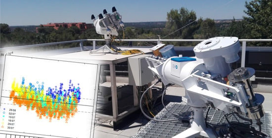
Both the primary reference ACR(s) and the standard pyrheliometer to be calibrated in Procedure A, or the standard reference REF pyrheliometer and the pyrheliometer under test DUT in Procedure B, are placed on a two-axis suntracking platform directly pointing towards the Sun disk. The readings of the output signal of the pyrheliometer(s) as well as some climatic variables (e.g., ambient and pyrheliometer temperatures, wind speed and direction, atmospheric pressure), are recorded in base intervals of 30 s by a data logging system and by a weather station at the calibration site.

In Procedure A, the solar irradiance provided by the primary radiometers is also synchronously registered by their control units (every 30 s in the case of an AHF, 90 s for a PMO6). During calibration or closed-phases of ACRs, data recorded from the pyrheliometer being calibrated are not used for responsivity calculation but for checking irradiance non-stability and tendency. When several ACRs (e.g., an AHF, passive-type and a PMO6, active-type) are combined, reference irradiance for coincident readings is the average of their individual estimations, but only if they differ in less than 0.5%. Otherwise, this irradiance value is rejected. In the case of non-coincident readings (that is, closed phase of AHF while PMO6 is measuring, or closed phase in PMO6 while AHF is measuring), or when only one ACR is being used for calibration, the irradiance given by the working ACR is taken as reference. Recording of experimental data is performed throughout the whole day, weather depending, and several days are used for a calibration (not necessarily consecutive).

In Procedure B, both REF and DUT pyrheliometers are measured synchronously because there are not intermittent open/closed phases. The instruments outputs are continuously recorded over several consecutive days, in an automated way, until enough valid data points are collected.

In both Procedure A and B, the final responsivity R is obtained as the average value:

$$R=\frac{1}{N}{\displaystyle \sum _{i=1}^{i=N}{R}_i},$$

(5)

of the individually calculated responsivities R_i from a set of N simultaneous measurements of irradiance E_i (by the ACR in Procedure A, of by the reference pyrheliometer in Procedure B) and the (DUT) pyrheliometer output signal V_i according to Equation (1) or Equation (3).

ISO 9059 and ASTM E816 standards suggest organizing or grouping the dataset in the form of series, by including experimental points recorded during periods of 10 to 20 min, and taking the responsivity as the average value of averages of different series. This approach makes sense for a statistical analysis of data points within a series, for example, to check for irradiance or signal stability, calculate standard deviation, etc. However, in the end, every one of the accepted, validated data points should contribute with the same statistical weight for the calculation of the responsivity. Therefore, in neither the PVLab Procedure A nor Procedure B, the measurements are divided in terms of series. All the data collected are analyzed and filtered (see below) in the same way, and all the points considered as valid have the same contribution to the computation of the final responsivity through Equation (5).

Additionally, in both Procedures A and B, the zero-irradiance offset δV₀ of pyrheliometers (output signal when irradiance is blocked, by covering their windows) is recorded during several hours at the beginning and/or end of the calibration campaign. This approach is discussed below. Cleaning of window surfaces of pyrheliometers is carried out on a daily basis during calibration campaign.

Acceptance criteria for validation of measured data are as follows:

• Abnormal values (negative values, NaN/blank lines, signal from shaded or overexposed sensor) are removed;
• Filtering due to weather conditions: irradiance E ≥ 700 W·m⁻²; Linke turbidity coefficient τ_L < 5.0; wind speed w_S < 3 m/s in any direction;
• Stability criteria: δE/δt ≤ ±1%/min for reference irradiance measured by ACRs, and of δV/δt ≤ ±1%/min for pyrheliometer output signal (equivalent to a variation of ≤0.5% in an interval of 30 s); individual points not in a contiguous stretch of six valid points are removed.

In both Procedures A and B, a minimum of 300 valid data points, for at least three different days, with no less than 10% of contribution of every day to the final dataset, are required. In addition, a distribution of [min 30%|max 70%] of data taken in the morning/in the afternoon are required in Procedure A, while a distribution of [min 40%|max 60%] of data are required for Procedure B.

2.4. General Approach for Computation of Uncertainty

The evaluation of uncertainty in the calibration of pyrheliometers here exposed follows the guidelines from the JCGM 100:2008 or GUM guide [57]. A few particular details are also common to the ASTM G213–17 standard. However, other methods for the computation of the uncertainty could also be suitable.

The objective is the calculation of the expanded uncertainty U(R_D), which is the value to be included in the calibration certificate together with the calculated responsivity R_D of the DUT pyrheliometer.

According to GUM, the combined standard uncertainty u_c(y) of any magnitude under evaluation y, calculated by a measurement function y = f (x₁, x₂, …, x_N) from the measured values x₁, x₂, …, x_N of some independent input variables, when they are no correlated to each other, is obtained as:

$$u_c^2(y)={\displaystyle \sum _{i=1}^n{\left[\frac{\partial f}{\partial x_i}\right]}^2{u}^2(x_i)},$$

(6)

where u(x_i) is the standard uncertainty of the input variable x_i and the partial derivatives are called sensitivity coefficients c_i.

Uncertainty u(x_i) contribution of each input variable can be evaluated either as A-type (statistical analysis of series of observations) or as B-type (means other than the statistical analysis of repeated observations, e.g., based on manufacturer’s specifications or data provided in calibration certificates). Additionally, depending on its nature, every uncertainty term u(x_i) is associated with a specific probability distribution (normal, rectangular, triangular, trapezoidal, etc.).

A-type uncertainty contributions u_A(x_i) are usually computed from a set of N experimental data points, treated as they were scattered according to a normal distribution. In the particular case of pyrheliometer calibration, uncertainty of the responsivity R obtained in Equation (5) is analyzed as an A-type contribution and then it is calculated as:

$$u_A^2\left(R\right)=\frac{{\sigma }^2\left(R\right)}{N}=\frac{1}{N\left(N-1\right)}{\displaystyle \sum }_{i=1}^{i=N}{\left(R_i-\mu \right)}^2,$$

(7)

where μ is the mean and σ(R) is the standard deviation of the individual responsivity R_i values taken as valid.

However, individual values of responsivity R_i are in turn determined with their own uncertainty u(R_i), each one calculated as a combined standard uncertainty in Equation (6). Addends in the quadratic sum Equation (6) will be evaluated as type-A or type-B depending on how they are originated, although most are B-type evaluations common to all the dataset. However, operating conditions (e.g., irradiance level, output signals, temperature, etc.) also affect the weight with which the uncertainty of each point contributes. The common practice in laboratories is using either the larger uncertainty of the dataset, or the value at some reference conditions (for example, in the case of pyrheliometers, this could be an irradiance of 1000 W·m⁻²). The alternative is to apply Monte Carlo methods of uncertainty evaluation [58]. In this work, the worst or most conservative case is considered (the larger relative uncertainty) and it can be demonstrated that this occurs for the lower output voltage (lower irradiance) in the range. The combined standard uncertainty of the responsivity of the pyrheliometer is, therefore, calculated by merging Equation (7) with that maximum value, and thus:

$$u^2\left(R\right)=u_A^2\left(R\right)+\max \left[u_c^2\left(R_i\right)\right],$$

(8)

Finally, this combined standard uncertainty u(R) is multiplied by a coverage factor k in order to obtain the final expanded uncertainty U(R) as:

$$U\left(R\right)=k·u\left(R\right).$$

(9)

based on the considered coverage probability. For k =2, and assuming a normal distribution function for R, the corresponding coverage probability is 95.45%. Any other coverage factor can be used (e.g., k = 1 for a probability of 68.27%), but the value of k applied (and the corresponding coverage factor) always has to be stated in the calibration certificate together with the value of the expanded uncertainty.

2.5. Uncertainty in the Calibration of Standard Pyrheliometers by Comparison to Cavity Radiometers (Procedure A)

Assuming there is no correlation between input variables, the combined standard uncertainty (6) of the responsivity according to the functional dependence of Equation (1), considering partial derivatives for the two input variables (E, V), would be:

$$\begin{array}{cc}{u}^2\left(R\right)\hfill & ={\left(\frac{\partial R}{\partial V}\right)}^2·u^2\left(V\right)+{\left(\frac{\partial R}{\partial E}\right)}^2·u^2\left(E\right)\hfill \\ & ={\left(\frac{1}{E}\right)}^2·u^2\left(V\right)+{\left(-\frac{V-V_0}{E^2}\right)}^2·u^2\left(E\right)\hfill \end{array}$$

(10)

It is more convenient to express Equation (10) in terms of relative uncertainty, by dividing all the terms in Equation (10) by R² in Equation (1):

$$\frac{u^2\left(R\right)}{R^2}=\frac{u^2\left(V\right)}{{(V-V_0)}^2}+\frac{u^2\left(E\right)}{E^2}$$

(11)

which gives the relative uncertainty of R in terms of those of V and E. Notice how the relative uncertainty depends on the measured values of output signal of the pyrheliometer being calibrated. Now, the contribution to uncertainty from every term in Equation (11) has to be evaluated.

2.5.1. Uncertainty Associated to Reference Irradiance

Irradiance is determined in Procedure A by the ACR measurement system considered as a whole instrument (including cavity sensing head, control electronics and measuring temperature, resistance, and voltage meters), according to its calibration. The calibration of the cavity system can be done well by characterization, that is, the calibration and/or evaluation of every magnitude of influence on its operating equation (its measurement merit function), or by direct comparison to the WSG (every 5 years during an IPC) or to one of the WSG members (usually, PMO2). In practice, the IPC comparison is the preferred option (the recommended practice by WMO) because of the huge complexity of the alternative calibration by characterization, beyond reach of most of the institutes owing and maintaining ACRs as their primary references.

As a result of this direct comparison during IPCs, every participating instrument receives a WRR transfer factor, F_WRR, a deviation or correction constant which should be applied by the ACR operator to reproduce the irradiance value that WSG would have given in the same location and operating conditions. This factor has associated a 1-σ standard deviation (expressed in ppm) and a number N of accepted values used for computing F_WRR, as published in the IPC reports [55,56].

Therefore, relative uncertainty associated to reference irradiance would be composed of these contributions:

$$\frac{u^2\left(E\right)}{E^2}=u^2\left(C_{SP}\right)+u^2\left(F_{WRR}\right)+u^2\left(\mathrm{WRR}\right)+u^2\left(\text{WRR-SI}\right)$$

(12)

which stand for the uncertainty u(C_SP) of the cavity radiometer specifications, that of the F_WRR factor u(F_WRR), the uncertainty u(WRR) of the WRR itself, and the uncertainty of the scale difference between WRR and SI units, u(WRR-SI). When the reference irradiance for calibration is obtained from the average value of irradiances measured by more than one cavity radiometer, every one adds its u(C_SP) and u(F_WRR) contributions to Equation (12) but u(WRR) and u(WRR-SI) have to be accounted for only once. Let us consider each term in Equation (12) separately.

First, it is accepted that WRR represents the physical units of total irradiance within 0.3% (with k = 3, a 99.73% certainty of the measured value) [28,54]. Then, the WRR uncertainty contribution in Equation (12) will be: u(WRR) = 0.3%/3 = 0.1%.

Second, uncertainty associated to F_WRR would be purely experimental, that is, A-type, and therefore, according to Equation (7), accounted for as: u²(F_WRR) = σ²/N.

Thus, in practice, it could be considered the quadratic sum: u² = u²(F_WRR) + u²(WRR), equivalent to the combined standard uncertainty obtained from a calibration certificate. In the case of using as reference a cavity radiometer that has not participated on an IPC yet, but has been traced and calibrated by comparison to another cavity radiometer, a correction factor F′ with an expanded uncertainty U(F′) and a coverage factor k should be given in its calibration certificate. In this case, the sum u²(F_WRR) + u²(WRR) in Equation (12) is substituted by u²(F′) = (U(F′)/k)².

After, the WRR-to-Si scale shift should be taken into account, but only if the results are to be referred to SI units, as expected by CIPM. When the calibrated responsivity of the pyrheliometer is only referred to WRR, as stated in the WMO technical regulations [54], this term is not required and u(WRR-SI) can be taken as zero in Equation (12). As commented, the discrepancy between scales is expected to be solved in the (near) future. However, in this transition period, while the scales are still to be aligned, both approaches would be compatible

Thus, when required, there are two possibilities for getting traceability of results to SI units via the WRR [46]:

• The user does not apply any correction factor for the scale difference and accepts a larger uncertainty of 0.3% (rectangular distribution), that is, u(WRR-SI) = 0.3%$/\sqrt{3}$;
• The user does apply the explicit correction factor F_SI for the scale difference of 0.336% (that is, by multiplying results by F_SI = 1/1.00336) and uses a smaller uncertainty contribution of 0.184% (with k = 2), that is: u(WRR-SI) = 0.092%.

The question is that nowadays all the laboratories involved in solar radiometry use WRR as reference, and applying the correction factor (0.336%) would introduce differences when results among different laboratories are compared. As before, the calibration certificate shall reflect whether the WRR-to-SI factor has been applied or not, and which is the reference used (WRR or SI). When the scales be aligned, probably no correction factor will be required and u(WRR-SI)~0.

Finally, like for any other measuring instrument, specifications of the cavity radiometer determining the accuracy of the irradiance measurements should be taken into account. In this sense, the ISO 9060:2018 standard included a new classification “Class AA”, pertinent to cavity radiometers, which is based on the same parameters as for standard pyrheliometers (e.g., zero-offset, tilt angle, non-linearity, non-stability, spectral effects, etc.) but with more restrictive limits. All these operational parameters are already taken into account in the specifications of standard pyranometers and pyrheliometers and for the evaluation of their uncertainty [39,41,43,59].

Therefore, this makes it necessary to consider these sources of uncertainty for the responsivity (or for the estimated irradiance) of cavity radiometers too. Although ISO 9060:2018 is not intended for calculation of uncertainty, the classification is indicative of how much deviation could be expected in a certain parameter or magnitude for an ACR. Moreover, it seems there is some lack of concretion in the standard because for most cavity radiometers a responsivity is not defined (e.g., a R_ACR given in V·W⁻¹·m²) but they have a correction factor such as F_WRR. However, it can be assumed that the irradiance provided by the radiometer could be affected in the same proportion as its responsivity.

Ideally, the manufacturer of a (new) ACR should provide the user with the performance characteristics of the instrument for these parameters to demonstrate conformance with the Class AA, in the same way as for standard pyrheliometers. However, in practice, most ACRs now in operation do not have to demonstrate conformance to that Class AA for being reference instruments, and do not have this set of specifications evaluated (in some cases, instruments are not currently on the market nor supported by their former, original manufacturers). Therefore, and in absence of these validation tests, it is convenient to de facto assume these Class AA ranges as the width of a confidence interval (rectangular distribution) for accounting for their possible impact into uncertainty. As will be seen later, in the end, these contributions are really small in the final uncertainty budget for a cavity radiometer.

Thus, accordingly, these relative contributions are grouped into the u(C_SP) uncertainty term as a quadratic sum:

$$u^2\left(C_{SP}\right)=u^2\left(\delta V_0\right)+u^2\left(ns\right)+u^2\left(nl\right)+u^2\left(\lambda \right)+u^2\left(T\right)+u^2\left(\theta \right)$$

(13)

where u(δV₀) refers to the uncertainty originated from the offset in the zero-irradiance signal, u(ns) is for non-stability of R_ACR (or equivalently, irradiance), u(nl) is for R_ACR non-linearity, u(λ) are due to spectral effects, u(Z) is the tilt response of R_ACR, u(T) is the temperature response, and u(ε) is due to additional processing errors.

2.5.2. Uncertainty Associated to the Measurement of Output Signal

Uncertainties of output signal u(V), originated by their measurement with a DMM, are calculated as:

$$u^2\left(V\right)=u^2\left(V_{SP}\right)+u^2\left(V_{CAL}\right)$$

(14)

including contributions from DMM calibration uncertainty u(V_CAL) and DMM specifications u(V_SP). The uncertainty associated to voltmeter specifications are instrument dependent, and can be composed, for example, of:

$$u^2\left(V_{SP}\right)=u^2\left(read\right)+u^2\left(T\right)+u^2\left(res\right)+u^2\left(conf\right)$$

(15)

accounting for possible contributions due to the reading or accuracy u(read), to a temperature coefficient u(T), to the resolution used u(res), and to other terms derived from the particular configuration u(conf) applied for measurement (e.g., integration time or NPLCs, use of analog or digital filters, input impedance, math null, noise influence, etc.). Alternative expressions can be developed for adapting u(V_SP) to different meters.

2.6. Uncertainty in the Calibration of Secondary Pyrheliometers against a Reference Standard Pyrheliometer (Procedure B)

In a similar way as for Procedure A, and assuming again there is no correlation between input variables, the combined standard uncertainty (6) of the responsivity calculated from Equation (3) would be:

$$\begin{array}{cc}{u}^2\left(R_D\right)\hfill & ={\left[\frac{\partial R_D}{\partial V_R}\right]}^2·u^2\left(V_R\right)+{\left[\frac{\partial R_D}{\partial V_D}\right]}^2·u^2\left(V_D\right)+{\left[\frac{\partial R_D}{\partial R_R}\right]}^2·u^2\left(R_R\right)\hfill \\ & ={\left[-\frac{V_D-V_{D0}}{{(V_R-V_{R0})}^2}{R}_R\right]}^2·u^2\left(V_R\right)+{\left[\frac{R_R}{V_R-V_{R0}}\right]}^2·u^2\left(V_D\right)+{\left[\frac{V_D-V_{D0}}{V_R-V_{R0}}\right]}^2·u^2\left(R_R\right)\hfill \end{array}$$

(16)

and dividing all the terms in Equation (16) by R² in Equation (3):

$$\frac{u^2\left(R_D\right)}{R_D^2}=\frac{u^2\left(V_D\right)}{{(V_D-V_{D0})}^2}+\frac{u^2\left(V_R\right)}{{(V_R-V_{R0})}^2}+\frac{u^2\left(R_R\right)}{R_R^2}$$

(17)

which gives the relative uncertainty of R in terms of those of V_R, V_D, and R_R. Now, the same term-by-term analysis as in the Equation (11) should be carried out, but first, two terms have contributions identical to those already calculated in Section 2.5.2. Observe that here uncertainty contributions from V measurements, u(V_D) and u(V_R), are also dependent on the output signals of both DUT and REF pyrheliometers.

Notice that the approach posed in Equations (16) and (17) is equivalent as considering Equation (1) as the measuring function, Equation (11) as its corresponding uncertainty, and the term u(E)/E, derived from Equation (2) for the reference pyrheliometer, as given by:

$$\frac{u^2\left(E\right)}{E^2}=\frac{u^2\left(V_R\right)}{{(V_R-V_{R0})}^2}+\frac{u^2\left(R_R\right)}{R_R^2}$$

(18)

The uncertainty of the DNI irradiance calculated by any pyrheliometer according to the simple expression Equation (2) is equivalent to Equation (18). Note also the parallelism between Equations (18) and (11).

With respect to the uncertainty u(R_R) associated to the responsivity of the reference pyrheliometer in Equation (17) or Equation (18), it would in turn be composed of:

$$u^2\left(R_R\right)=u^2\left(P_{SP}\right)+u^2\left(P_{CAL}\right)$$

(19)

taking into account contributions due to the calibration u(P_CAL) of the reference pyrheliometer and to instrument specifications u(P_SP). These instrument specifications or class-based contributions are also associated to its ISO 9060:2018 classification. Then, uncertainty u(P_SP) can be expressed, like in Equation (13), as:

$$u^2\left(P_{SP}\right)=u^2\left(\delta V_0\right)+u^2\left(ns\right)+u^2\left(nl\right)+u^2\left(\lambda \right)+u^2\left(T\right)+u^2\left(Z\right)+u^2\left(\epsilon \right)$$

(20)

where, similarly, uncertainty contributions arise from offset in the zero-irradiance signal u(δV₀), non-stability of R_R u(ns), R_R non-linearity u(nl), spectral effects u(λ), tilt response of R_R u(Z), temperature response u(T), and additional processing errors u(ε).

However, the difference is that, in the case of standard pyrheliometers (Class A, for example), specifications are usually given in the instructions’ manual by the manufacturer, because this is the common practice since the issue of the former ISO 9060:1990 edition. If any of the specifications is not explicitly given in the manual, it could either be (experimentally, numerically, by simulation) evaluated by the user or it could be accounted for by using the ISO 9060:2018 bounds for that parameter in the corresponding class stated by the manufacturer for that instrument. Notice that some of the contributions in Equation (19) could be null or zero, depending on the particular setup and the characteristics of the reference pyrheliometer. For example, u(ε) = 0 for a passive-type pyrheliometer with no electronics embedded.

Alternatively, correction terms for every one of the magnitudes of influence included in Equation (19) can be introduced into Equation (1) for a finer evaluation of irradiance E by the reference pyrheliometer. There are, therefore, two options:

• A particular correction is explicitly used for evaluating E; then, Equations (1), (17) and (18) are accordingly modified, and the uncertainty of the correction is computed independently in Equations (17) and (18), out from Equation (20), on the basis of the method used; or
• That correction is not applied for estimating E; then, the corresponding uncertainty that this magnitude introduces in the estimation of E by the reference pyrheliometer is taken into account as in Equation (20).

Appendix A provides a general approach to consider further correction terms, and how the responsivity and DNI irradiance and their uncertainties could be calculated.

On the other hand, u(P_CAL) is easy to be computed because it is based on the calibration certificate of the reference pyrheliometer (obtained internally through Procedure A, given by an external calibration laboratory). Again, provided the calibrated responsivity is given in a certificate with its standard expanded uncertainty U(R_R) and a certain coverage factor k, we get: u(P_CAL) = U(R_R)/k.

Finally, for pyrheliometers with 4–20 mA current loop output signals which are measured through a shunt resistor R_SH, it can be demonstrated that the relative uncertainty corresponding to Equation (4) would be:

$$\frac{u^2\left(R_D\right)}{R_D^2}=\frac{u^2\left(R_{SH}\right)}{R_{SH}^2}+\frac{u^2\left(V_D\right)}{{(V_D-V_{D0})}^2}+\frac{u^2\left(V_R\right)}{{(V_R-V_{R0})}^2}+\frac{u^2\left(R_R\right)}{R_R^2}$$

(21)

instead of Equation (17). Then, the addition of the new term u(R_SH)/R_SH would in turn consist of a term U(R_SH)/k from its calibration and a term corresponding to its specifications.

3. Results

The methodology explained in Section 2 is applied now to the calibration of a Class A reference standard pyrheliometer by comparison to a cavity radiometer (Procedure A) and of a Class A pyrheliometer by comparison to that Class A reference standard pyrheliometer (Procedure B). Thus, the Class A pyrheliometer calibrated with Procedure A serves after as the reference instrument in Procedure B. The ISO 9059:1990 standard allows calibrating pyrheliometers by comparison to reference pyrheliometers of the same or higher class.

In both cases, the experimental values of the responsivity for each device, once the process of analysis and filtering is completed, are shown. Then, the calculation of the uncertainty terms is explained, with the results summarized in the form of tables. The final result is shown in graphs where the different approaches (due to the duality of reference scales and the ways to account their respective uncertainties) are compared.

In addition, the reader should be aware that results here shown are particular of PVLab-CIEMAT instruments, sensors and meters, while equations in Section 2 are of general application.

3.1. Procedure A: Calibration of a Class A Standard Pyrheliometer against a Cavity Radiometer

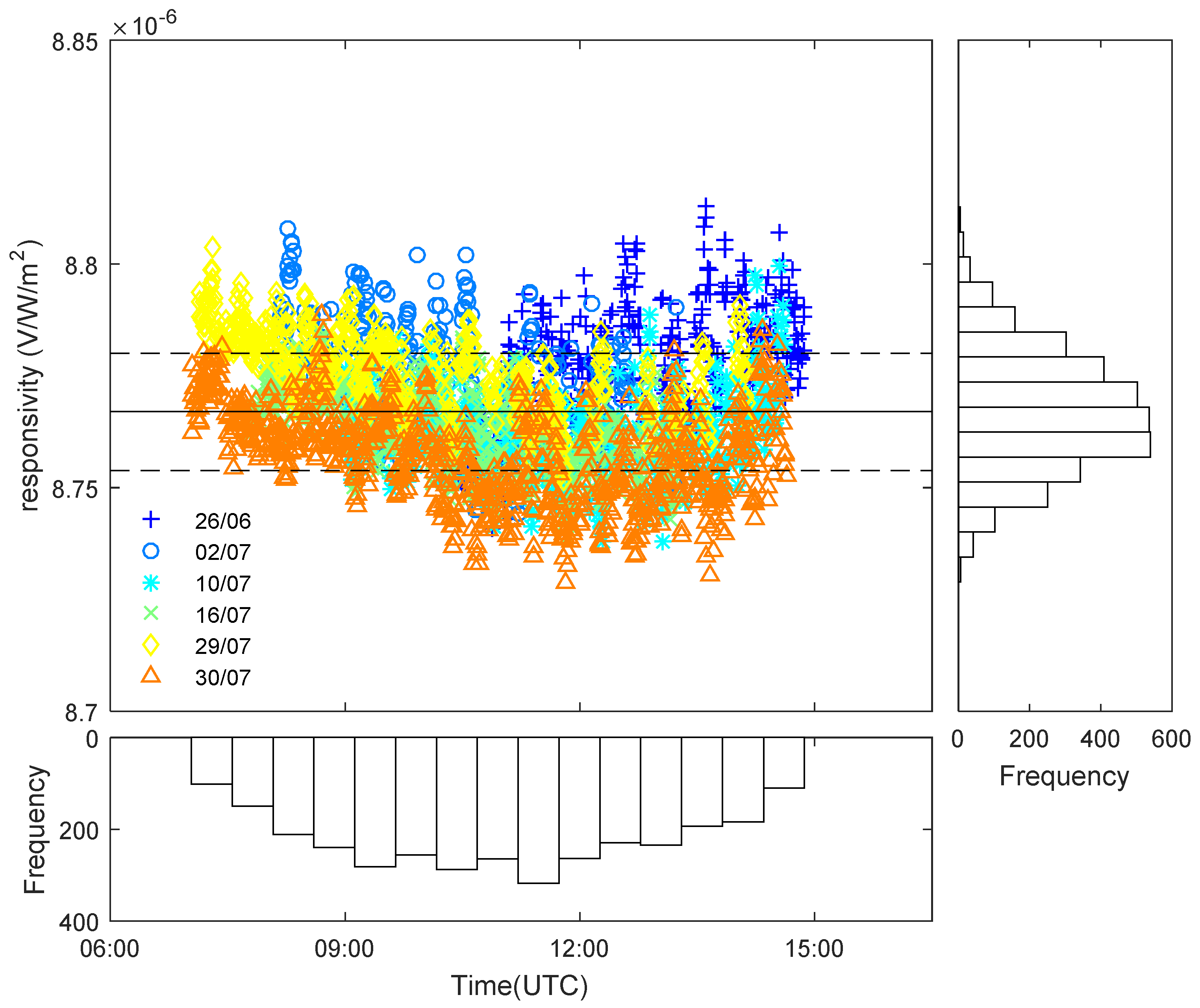
Figure 2 shows the responsivity of a Class A reference standard pyrheliometer obtained by comparison outdoors to our cavity radiometer model Eppley AHF SN 28,486 according to Procedure A, which conforms to ISO 9059:1990 standard. The Class A instrument is a passive type, thermopile-based, nominal V₀ = 0 mV signal at zero-irradiance conditions, and an internal 10 kΩ thermistor as temperature sensor. Readings have not been corrected in temperature. When the calibrations results are referred to WRR, as usual, the responsivity obtained is: R = (8.767 ± 0.020) μV·W⁻¹·m² (k = 2).

How has this U uncertainty figure been obtained?

Table 1. Classification of Class AA pyrheliometers (ISO 9060) and estimated contribution to u(C_SP) due to ACR specifications in Equation (13).

Term	Parameter	Specification	Stat. Distrib.	Relat. Contrib.	Net Contrib.
u(δV0)	Zero offset: response to ΔTAMB = 5 K·h−1	±0.1 W·m−2	Rectangular	143 × 10−6$/\sqrt{3}$	82 × 10−6
u(ns)	Non-stability (variation per year)	±0.01%	Rectangular	$0.01\%/\sqrt{3}$	58 × 10−6
u(nl)	Non-linearity	±0.01%	Rectangular	$0.01\%/\sqrt{3}$	58 × 10−6
u(λ)	DNI spectral error	±0.01%	Rectangular	$0.01\%/\sqrt{3}$	58 × 10−6
u(T)	Temperature response	±0.01%	Rectangular	$0.01\%/\sqrt{3}$	58 × 10−6
u(Z)	Tilt response	±0.01%	Rectangular	$0.01\%/\sqrt{3}$	58 × 10−6
u(ε)	Additional signal processing errors	±0.1 W·m−2	—	—	—
	Total relative u(CSP)				153 × 10−6

,

Table 2. Estimated relative uncertainty u_B(E)/E of the reference irradiance from Equation (12).

Term	Parameter	Contribution	Net Contr. (WRR)	Net Contr. (SI)
u(CSP)	ACR/Class AA specifications	(see Table 1)	153 × 10−6
u(FWRR)	WRR factor, IPC-XII (2015)	$\sigma /\sqrt{N}$	38 × 10−6
u(WRR)	Uncertainty of WRR (U = 0.3%, k = 3)	0.3%/3	1000 × 10−6
u(WRR-SI)	Uncertainty of WRR-to-SI shift	$0.3\%/\sqrt{3}$	—	1732 × 10−6
	Total u(E)/E		1012 × 10−6	2006 × 10−6

,

Table 3. Contributions to uncertainty from voltmeter specifications according to Equation (15).

Term	Parameter, Value	Statis. Distr.	Net Contribution
u(read)	Reading or accuracy: rng = 100 mV	Rectangular	405 × 10−6
u(T)	T coefficient for T outside 23 ± 5 °C: T = 23 °C, rng = 100 mV	Rectangular	—
u(res)	Resolution: 6½ digits, LSD = 10−7 V	Rectangular	5 × 10−6
u(conf)	Additional configuration-derived errors	Rectangular	—
	Total u(VSP)/(V–V0)		405 × 10−6

,

Table 4. Contributions to uncertainty in voltage measurements according to Equation (14).

Term	Parameter	Value	Contribution	Net Contribution
u(VSP)	Voltmeter specifications		(see Table 3)	405 × 10−6
u(VCAL)	Calibration uncertainty U (k = 2)	U = 6.4 × 10−7 V	(U/k)/(V–V0)	52 × 10−6
	Total u(V)/(V–V0)			409 × 10−6

and

Table 5. Final computation of net expanded uncertainty in the calibration of Class A pyrheliometer according to Procedure A.

Relative Uncertainty Term	Expression	Equation	Contrib. (WRR)	Contrib. (SI)
V measurements of DUT	$u\left(V\right)/\left(V-V_0\right)$	(14)	409 × 10−6
Reference irradiance	$u\left(E\right)/E$	(12)	1012 × 10−6	2006 × 10−6
Relative combined uncertainty	$u_c\left(R\right)/R$	(11)	1092 × 10−6	2047 × 10−6
Relative type-A uncertainty	$u_A\left(R\right)/R$	(7)	<300 × 10−6
Relative combined uncertainty	$u\left(R\right)/R$	(8)	1132 × 10−6	2069 × 10−6
Relative expanded uncertainty (k = 2)	$U\left(R\right)/R=k·u\left(R\right)/R$	(9)	2264 × 10−6 (0.23%)	4139 × 10−6 (0.41%)

collect all the steps for the application of the method of Section 2.5, in particular, Equations (11)–(15).

In Table 1, estimated contributions from different sources to u(C_SP) in the irradiance measured by an ACR, according to Equation (13), are computed. Limits of the classification for Class AA pyrheliometers in ISO 9060:2018 have been used for this. Relative contribution of δV₀ is referred to 700 W·m⁻², the lower irradiance allowed during calibrations, because the largest uncertainty is obtained for the lowest irradiance. Contributions are expressed in terms of ×10⁻⁶ instead of ppm, following the recommendation of the ILAC P14:09 [60].

In Table 2, Equation (12) is evaluated. F_WRR factor of Eppley AHF 28,486 cavity radiometer obtained in the last IPC-XII (2015) is used for this calibration (F_WRR = 0.997318, N = 280, 1σ = 0.000629). Two relative uncertainty values of u(E)/E, one for R only referred to WRR, the other including the WRR-SI larger uncertainty, have been calculated for comparison. The third option, correcting R to SI and using U = 0.184% (k = 2), gives a relative uncertainty u(E)/E = 1368 × 10⁻⁶. This has not been included in Table 2 for clarity.

Table 3 and Table 4 show the calculation of Equations (15) and (14), respectively. A reading of V ≈ 6.14 mV is approximately given at 700 W·m⁻² for this pyrheliometer with R = 8.767 μV·W⁻¹·m², and V₀ = 0 mV. Remember relative u(V)/(V–V₀) is dependent on V–V₀ values. Contributions in Equation (15) are associated to the specifications of the Agilent 34970 A datalogger used as recording instrument: u(read) = (0.005% × V + 0.004% × range)$/\sqrt{3}$ V; resolution term with a Last Significant Digit (LSD) value is u(res) = (LSD/2)$/\sqrt{3}$ V; temperature coefficient is u(T) = (0.0005% × V + 0.0005% × range)$/\sqrt{3}$ °C⁻¹ but only for T outside the range 23 ± 5 °C; and the rest of DMM parameters are set as to not introduce additional uncertainty penalties (e.g., integration time NPLC = 10). Calibration certificate of the data-logger gives an uncertainty of U = 6.4 × 10⁻⁷ V (k = 2) for readings of ±10 mV.

The combined standard and expanded uncertainties, with all these contributions taken into account, are collected in Table 5. Again, two uncertainty figures have been presented, with R referred to WRR and with WRR-SI uncertainty. The other possibility, correcting R to SI by applying the factor F_SI, gives u(R)/R = 1459 × 10⁻⁶ and U(R)/R = 2918 × 10⁻⁶. Thus, the final value referred to SI would be R = (8.735 ± 0.026) μV·W⁻¹·m² (k = 2).

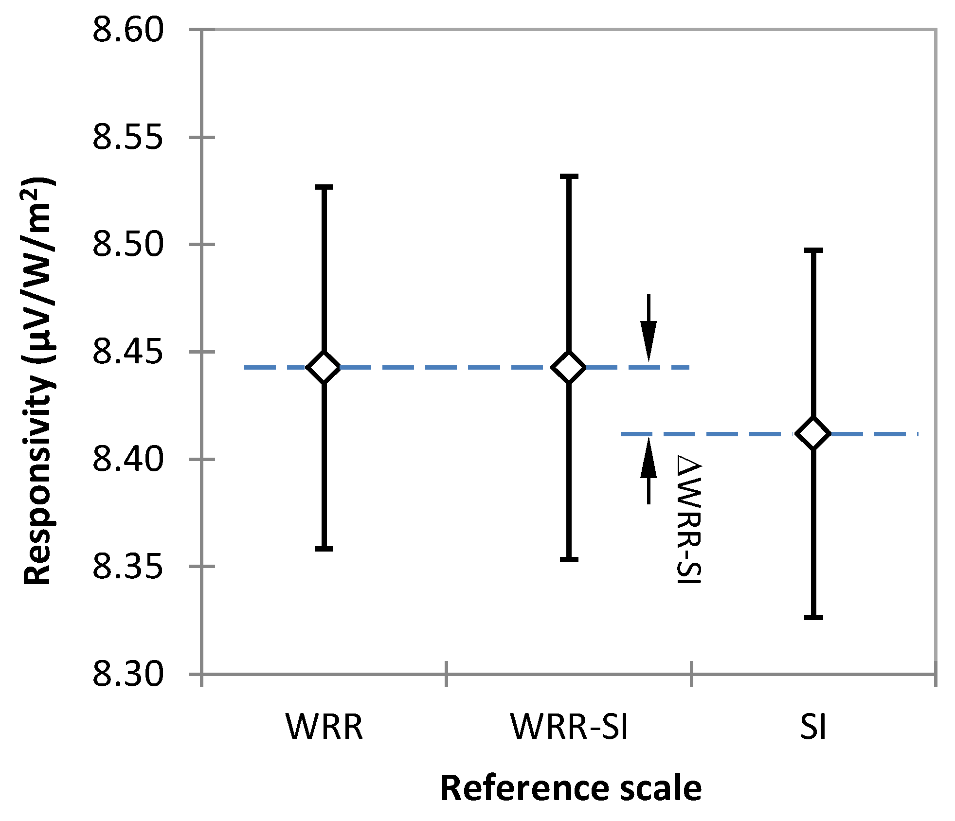
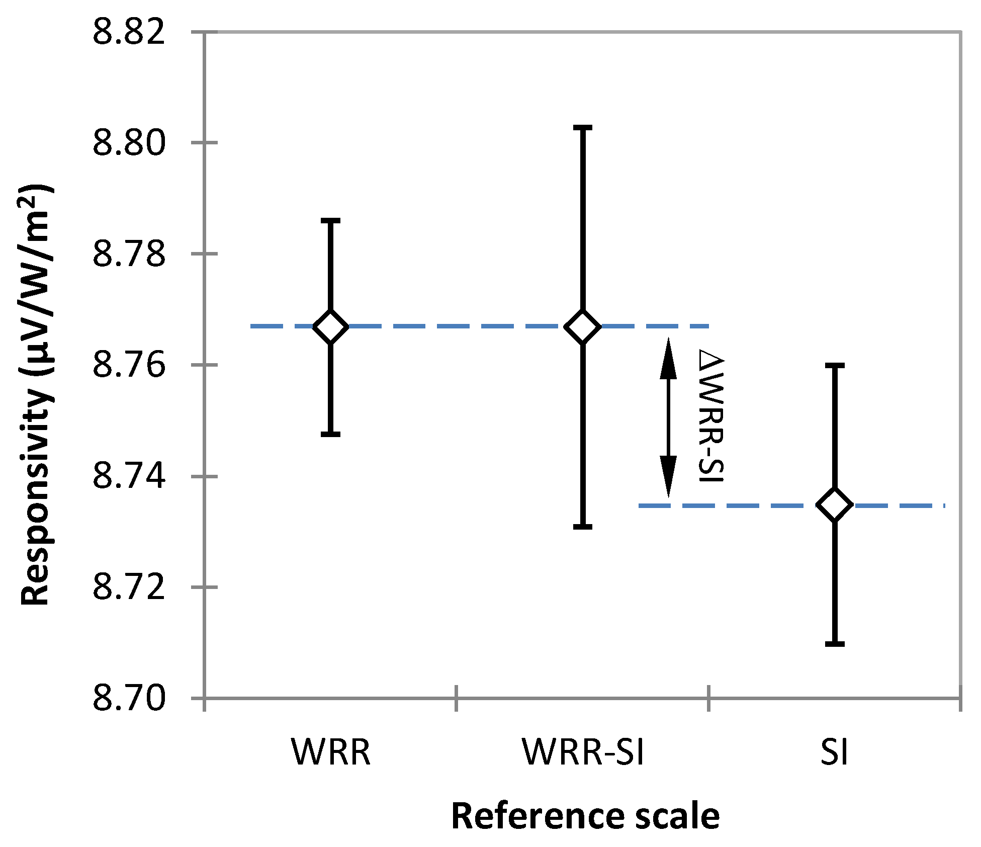
Figure 3 plots the values of the responsivities and uncertainties that are obtained with the three approaches described above.

As seen in Figure 3, current shift between WRR and SI scales gives as result a difference in responsivity and uncertainty values that can create confusion and that makes the alignment between scales recommendable (and necessary) in the short term.

It is also important to evaluate the relative weights that the different terms have in the net combined uncertainty. In this case, reference irradiance u(E)/E represents ~80% of the uncertainty budget when the results are referred to WRR, while it represents ~94% if they include the uncertainty of the WRR-SI shift. In fact, ~70% of the 2069 × 10⁻⁶ uncertainty is due to the WRR-SI shift uncertainty. Moreover, the uncertainty associated to the Class AA specifications represents less than 2% for WRR and less than 0.6% for WRR-SI figures.

3.2. Procedure B: Calibration of a Class A Standar Pyrheliometer by Comparison to a Class A Reference Pyrheliometer

The Class A reference pyrheliometer calibrated as described in Section 3.1 has been used for calibrating another Class A secondary pyrheliometer following Procedure B. This second Class A instrument is also a passive type, thermopile-based, nominal V₀ = 0 mV signal at zero-irradiance, but without an internal temperature sensor. Figure 4 plots the results obtained in the calibration of the DUT pyrheliometer. The responsivity obtained in this case, referred to WRR, was: R = (8.443 ± 0.085) μV·W⁻¹·m² (k = 2).

The procedure for calculating the uncertainty is similar to the case of Procedure A, but now it is based on Equations (17)–(20) of Section 2.6 and Equations (14) and (15) of Section 2.5. The results of all these calculations are compiled in

Table 6. Classification of Class A pyrheliometers (ISO 9060) and estimated contribution to u(P_SP) due to device specifications in Equation (20).

Term	Parameter	Specification	Statis. Distrib.	Relative Contr.	Net Contr.
u(δV0)	Complete zero offset	±2 W·m−2	Rectangular	2857 × 10−6$/\sqrt{3}$	1650 × 10−6
u(ns)	Non-stability (ΔR/year)	±0.5%	Rectangular	$0.5\%/\sqrt{3}$	2887 × 10−6
u(nl)	Non-linearity of R	±0.2%	Rectangular	$0.2\%/\sqrt{3}$	1155 × 10−6
u(λ)	Clear sky DNI spectral error	±0.2%	Rectangular	$0.2\%/\sqrt{3}$	1155 × 10−6
u(T)	Temperature response of R	±0.5%	Rectangular	$0.5\%/\sqrt{3}$	2887 × 10−6
u(Z)	Tilt response of R	±0.2%	Rectangular	$0.2\%/\sqrt{3}$	1155 × 10−6
u(ε)	Additional processing errors	±1 W·m−2	—	—	—
	Total relative u(PSP)				4836 × 10−6

,

Table 7. Estimated relative uncertainty u_B(R_R)/R_R of the reference pyrheliometer from Equation (19).

Term	Parameter	Value	Contribution	Net Contrib.
u(PSP)	Instrument specifications	(see Table 6)		4836 × 10−6
u(PCAL)	Calibration uncertainty U (k = 2) RR = 8.767 μV·W−1·m2	(see Table 5)	(U/k)/RR	1132 × 10−6 2069 × 10−6
	Total u(RR)/RR		(WRR) (SI)	4967 × 10−6 5260 × 10−6

,

Table 8. Contributions to uncertainty from voltmeter specifications according to Equation (15). See text for further details.

Term	Parameter, Value	Statis. Distr.	DUT	REF
u(read)	Reading or accuracy: rng = 100 mV	Rectangular	421 × 10−6	405 × 10−6
u(T)	T coefficient for T outside 23 ± 5 °C: T = 23 °C, rng = 100 mV	Rectangular	—	—
u(res)	Resolution: 6½ digits, LSB = 10−7 V	Rectangular	5 × 10−6	5 × 10−6
u(conf)	Additional configuration-derived errors	Rectangular	—	—
	Total u(VSP)/(VX–VX0)		421 × 10−6	405 × 10−6

,

Table 9. Contributions to uncertainty in voltage measurements according to Equation (14).

Term	Parameter	Value	Contribution	DUT	REF
u(VSP)	Voltmeter specifications		(see Table 8)	421 × 10−6	405 × 10−6
u(VCAL)	Calibration uncertainty U (k = 2)	U = 6.4 × 10−7 V	(U/k)/(VX–VX0)	55 × 10−6	53 × 10−6
	Total u(VX)/(VX–VX0)			424 × 10−6	409 × 10−6

and

Table 10. Final computation of net expanded uncertainty with different contributions referring to WRR and SI.

Relative Uncertainty Term	Expression	Equation	Contrib. (WRR)	Contrib. (SI)
V measurements of DUT	$u\left(V_D\right)/\left(V_D-V_{D0}\right)$	(14)	424 × 10−6
V measurements of REF	$u\left(V_R\right)/\left(V_R-V_{R0}\right)$	(14)	409 × 10−6
REF specifications and calibration	$u\left(R_R\right)/R_R$	(19)	4967 × 10−6	5260 × 10−6
Relative combined uncertainty	$u_c\left(R_D\right)/R_D$	(17)	5002 × 10−6	5293 × 10−6
Relative type-A uncertainty	$u_A\left(R_D\right)/R_D$	(7)	<500 × 10−6
Relative combined uncertainty	$u\left(R_D\right)/R_D$	(8)	5026 × 10−6	5317 × 10−6
Relative expanded uncertainty (k = 2)	$U\left(R_D\right)=k·u\left(R_D\right)$	(9)	10,053 × 10−6 (1.01%)	10,633 × 10−6 (1.06%)

. Now, the description of some steps and Tables is easier because in some cases the computation process is near identical as for Procedure A (Section 3.1).

Contributions due to the specifications of the reference pyrheliometer, according to Equation (20), have been listed in Table 6. In this case, specifications for Class A pyrheliometers in ISO 9060:2018 have been used. Observe that specifications given by the manufacturer in the instructions’ manual of pyrheliometer should be used instead of Class A specification in Table 6. Today, many pyrheliometers on the market can significantly exceed the requirements of Class A in several of these classification parameters. Therefore, values in Table 6 should be understood as the maximum a Class A pyrheliometer could contribute for every parameter for computation of u(P_SP). Again, absolute contributions are converted into relative ones by using 700 W·m⁻², the lower irradiance allowed for data points in the calibration Procedure B.

In Table 7, responsivity and uncertainty values obtained by the reference pyrheliometer calibrated in Section 3.1 (Table 5) have been used for calculating u(R_R)/R_R. Here, the two ways to account uncertainty (only WRR and WRR-SI) have also been presented, as in Table 5. The corresponding figure when correcting R to SI is u(R_R)/R_R = 5051 × 10⁻⁶.

Table 8 and Table 9 are quite similar to Table 3 and Table 4 in Section 3.2. Now, readings of V_D ≈ 5.9 mV and V_R ≈ 6.14 mV (approximate values at 700 W·m⁻² of a DUT with R_D = 8.443 μV·W⁻¹·m² and REF R_D = 8.767 μV·W⁻¹·m²) and zero-irradiance V_D0 = 0, V_R0 = 0 values have been used. Computation of u(V_SP)/(V_X–V_X0) in Table 8 follows the same idea as in Table 3, but in separate amounts for DUT and REF devices. The same value from calibration certificate as in Table 4 has been used in Table 9.

The final computation of the combined and expanded uncertainties is covered in Table 10. Following the same criteria, uncertainties with R referred to WRR and with WRR-SI uncertainty are given. Correcting R to SI with the factor F_SI produces u(R_D)/R_D = 5086 × 10⁻⁶ and U(R_D)/R_D = 10220 × 10⁻⁶ (1.02%). Moreover, the final value corrected to SI would be: R = (8.412 ± 0.086) μV·W⁻¹·m² (k = 2).

As before, the values of the responsivities and uncertainties obtained with the three approaches (WRR, WRR-SI and SI) are represented in Figure 5. The proportion among the uncertainty bars (k = 2) in the three cases is now very similar, while they were appreciably different in Figure 3. Moreover, the relative size of these uncertainty bars with respect to F_SI (being the same factor as in Figure 3) is now larger. This is a clear effect of how uncertainty is being increased in the transfer of WRR scale in each calibration.

The main reason for this difference is the greater contribution of the instrument specifications u(P_SP)/R_R in u(R_R)/R_R (Equation (19), Table 6 and Table 7). Now, the specifications of the reference pyrheliometer (4836 × 10⁻⁶) have a weight of about ~93% in the total uncertainty budget in the case of R is referred to WRR, of about ~83% when including the WRR-SI shift uncertainty, and about ~90% when the correction to SI is applied. In comparison, calibration uncertainty u(P_CAL)/R_R represents only around ~5% in the first case, ~15% in the second one, and around ~8% when the correction to SI is applied.

On the other hand, notice how the uncertainty assigned to A-type uncertainty is low in both Table 5 and Table 10. In these calibrations of Class A instruments, the influence of external magnitudes of influence (despite their uncertainty) is in general small, even more if the REF and DUT pyrheliometers are of the same brand and model, and this results in obtaining relatively uniform sets of responsivity data points. Moreover, as, once filtered, the number of valid points is usually large (N > 1000) and the statistical standard deviation σ is small (σ/R < 0.5%), the relative weight of A-type uncertainty (7) in the total uncertainty budget is negligible.

3.3. Influence of the Temperature of Operation

In many cases, instruments of use in monitoring systems or weather stations are not Class A pyrheliometers and the influence of working conditions (as some parameters reflected in Table 1 and Table 6) is larger, and these can affect the calibration results and later the quality of the DNI irradiance measured. One example of such an influence, that is relatively easy to record and analyze, is the operating (ambient or instrument) temperature.

Recording the operating temperature T of all DUT pyrheliometers (whatever their class), simultaneously with their output signals, has been adopted in PVLab-CIEMAT as a common practice in routine calibrations (both in Procedures A and B). The measurement of temperature makes it easier to analyze potential deviations on the calibration results, and to estimate the dependence of responsivity on T. Curiously, while ISO 9847:1990 considers the possibility of correcting responsivity values to a reference temperature T₀ (not specified in the standard) for pyranometers, ISO 9059:1992 does not include this option for pyrheliometers.

The dependence of responsivity on T was expressed in ISO 9847:1990 by means of a linear model and a relative thermal coefficient α_R in the form:

$$R\left(T_0\right)=\frac{R\left(T\right)}{1+{\alpha }_R·\left(T-T_0\right)}$$

(22)

where α_R is given in °C⁻¹ or K⁻¹ (coherently with T). Other expressions, by using a second- or third-degree polynomial on T are also referred in the literature [61]. According to our experience, and for the usual range of temperatures in our facilities during the year, responsivity of pyrheliometers follows a similar mathematical model as Equation (22) and it can also be used for correcting their responsivities as well as to calculate the relative thermal coefficient. Although choosing a reference temperature T₀ of universal application is difficult, ISO 9060:2018 indirectly refers to T₀ = 20 °C when setting the classification criteria for temperature response of both pyranometers and pyrheliometers. For this reason, and for being a common working temperature in our facilities, T₀ = 20 °C is taken as set point in PVLab for these calculations.

For pyrheliometers not having an internal T sensor (usually a 10 kΩ thermistor or a Pt100 whose terminals are accessible through the cable/connector), an external Pt1000 is externally adhered to the body of the pyrheliometer in such a form that solar irradiance does not impinge directly on the T sensor. While temperature measured by the internal sensor can be much more realistic (it is close to the irradiance sensing element), it is difficult to know its calibration parameters (range, deviation, uncertainty, etc.). On the contrary, external sensor can be carefully calibrated, but the temperature is that of the body of the pyrheliometer, which can be different from the one of the irradiance sensor.

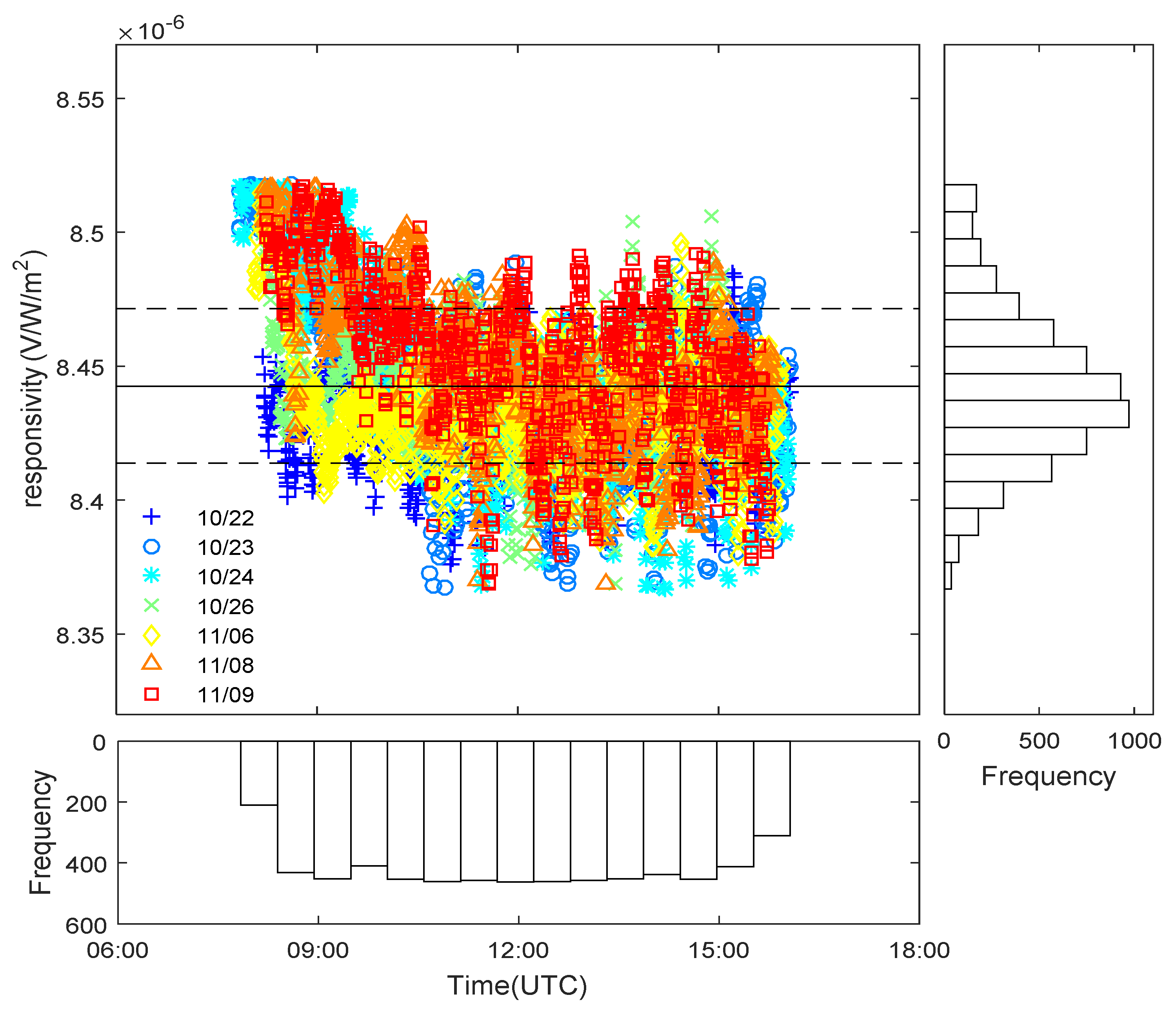
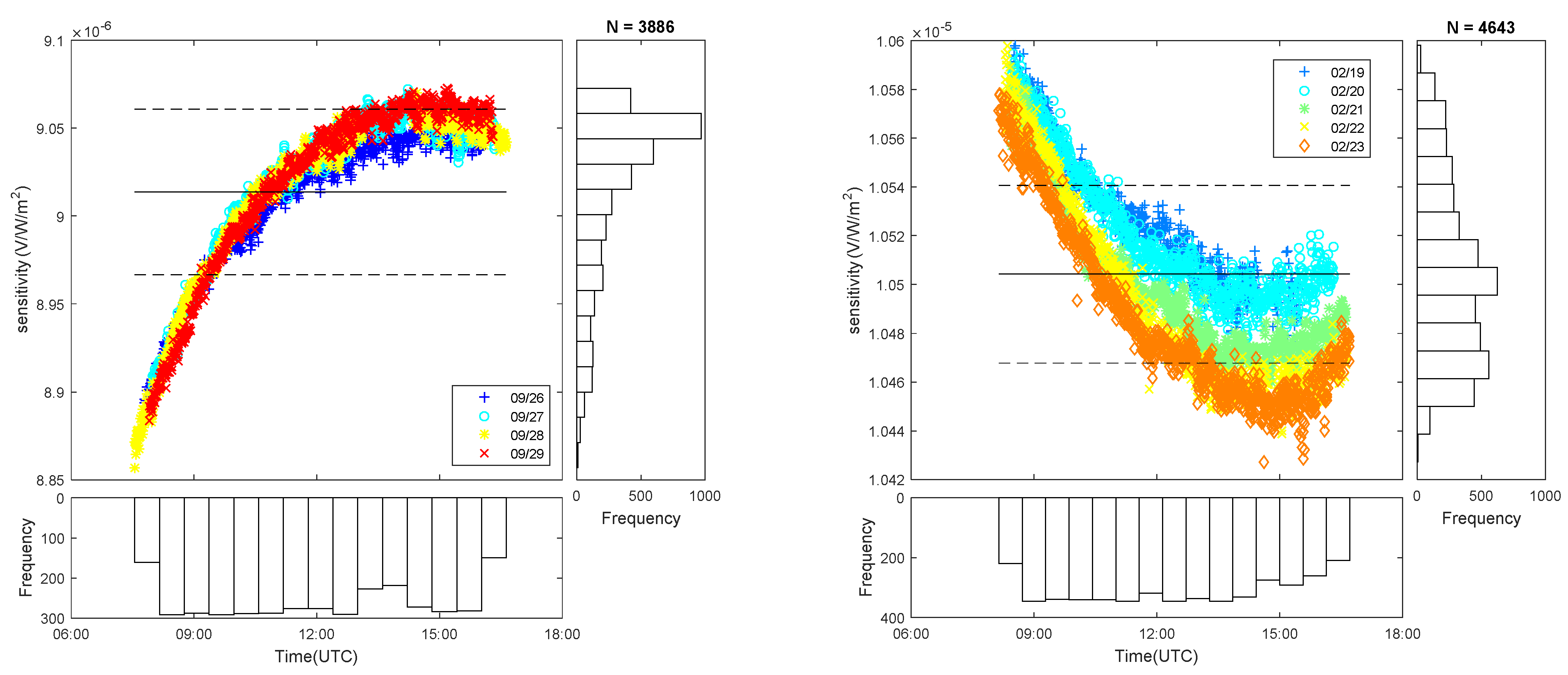
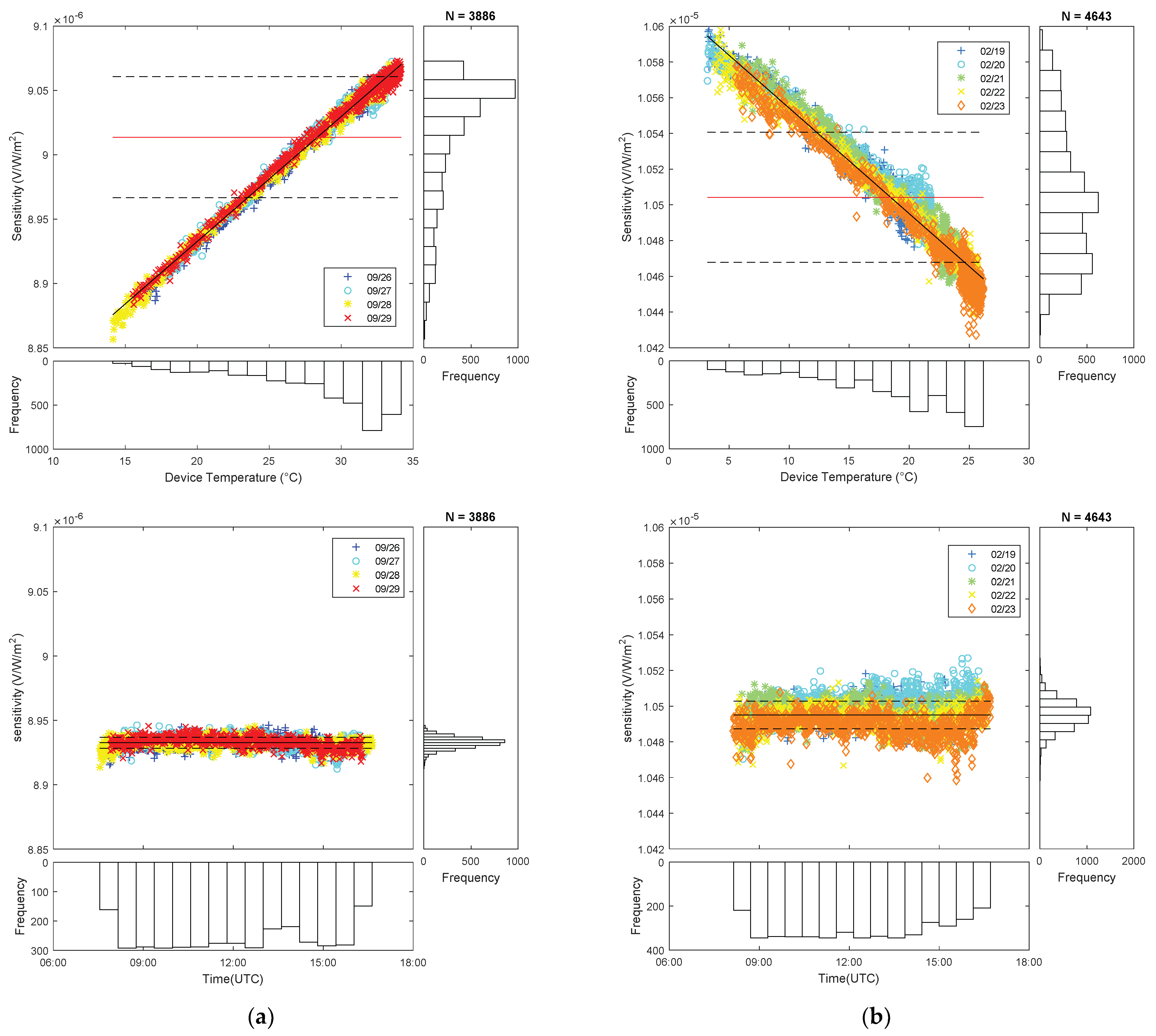
Figure 6 shows an example of the responsivity obtained during the calibration of two different Class B pyrheliometers, once data are analyzed and filtered (low irradiance, abnormal values, unstable periods, etc.). This is not a general behavior—these are particular cases selected for illustrating the problems in the calculation of responsivity and the possibilities of this correction method on temperature. Importantly, pyrheliometer (a) was calibrated in September with operating temperatures between 15 °C to near 35 °C, while pyrheliometer (b) was calibrated in February with temperatures between 5 °C to 25 °C. It can be seen how the responsivity varies during the day, and for different days, for both instruments but in opposite directions.

Due to the natural evolution of ambient temperature during the day, these behaviors lead to think on a temperature dependence of responsivity. The second row of graphs in Figure 6 confirms this relationship R(T) and shows how an approximate thermal coefficient α_R can be calculated from the slope of a least squares fit to a straight line. Afterwards, responsivity has been corrected to T₀ = 20 °C by using Equation (22) and the α_R coefficient obtained in the previous step. Results are shown in the last row of Figure 6. It can be seen how, for these cases, more homogeneous and stable responsivity values are obtained, and with reduced standard deviations σ. Numerical results, with the responsivities obtained at reference temperature and the differences to initial values, are summarized in

Table 11. Comparison between results for the pyrheliometers, whose responsivity is affected by a strong temperature dependence, taken as a case study. Values of R(T₀) are for T₀ = 20 °C.

Parameter	Pyrheliometer (a)	Pyrheliometer (b)
Valid data (N)	3886	4643
Average T along calibration campaign	27.85 °C	18.44 °C
R without T correction, R(T) (μV·W−1·m2) [standard deviation]	9.0137 [σ = 0.0471]	10.504 [σ = 0.0364]
R with T correction, R(T0) (μV·W−1·m2) [standard deviation]	8.9326 [σ = 0.0042]	10.495 [σ = 0.0077]
Approximate αR (°C−1)	+1.09 × 10−3	−5.63 × 10−4
Approximate temperature response according to ISO 9060:2018 (between −10° to +40 °C)	5.44%	2.81%

.

The main unknowns here are which responsivity value shall be stated in the calibration certificate and at which reference conditions. As this is not regulated in standards, the average responsivity as calculated by Equation (5) in the above Procedure B is stated in the certificate, according to ISO 9059, without any T correction, and the client is informed about these findings. However, developing a correction procedure for these cases, or at least a reference temperature of common use, to be suggested in the standards, would be interesting, even if used only as an informative or recommended practice. This would also help for comparisons among responsivities obtained in different weather conditions, in different years, or by different laboratories. It would also be convenient suggesting to manufacturers to always include a temperature sensor in their radiometers for these purposes.

4. Discussion

Although some comments have already been introduced in Section 2 and Section 3, specific points deserve additional comments.

First, uncertainties obtained in this work are consistent although slightly lower than values reported in the literature (with k = 2) for calibration of pyrheliometers (Procedure B): 1.4% [43], 1.8% [44], 1.9–2.7% [38,41], 2–3% [42], and slightly lower than values obtained in calibration by reference laboratories (Procedure A): 0.25–0.39% [62]. It is possible that a higher contribution of A-type component, or additional terms missed in our analysis, could explain these differences.

On the other hand, it seems recommendable that the gap between WRR and SI radiometry scales be corrected or aligned soon, in order to avoid the differences found between the responsivities and uncertainties as in this work. However, the shift is more relevant for calibration of higher-class instruments than in lower stages of the WRR traceability chain, because the uncertainty in successive WRR transfers increases to a point in which the WRR-SI gap becomes imperceptible. When the DNI irradiance is later determined by the DUT pyrheliometer, the WRR-SI discrepancy will probably have an even lower impact because the DUT specifications are combined with its calibration uncertainty for obtaining that of solar irradiance. Moreover, in the end, in terms of uncertainty, there will not be a difference between using WRR or SI as reference.

Uncertainties given in calibration certificates cannot be modified by the end users to account for additional uncertainty terms or in order to remove them. If the calibration laboratory did not include these quantities, the u(WRR-SI) cannot be added by the user to the certified uncertainty, nor can the calibrated responsivity be multiplied by the F_SI factor, to refer the radiometric data to SI, for example. If desired, end users should request to the laboratory to refer the results to SI in order to correctly integrate uncertainty and correction factor in their results.

Additionally, it is also important to identify where a correction term (and its uncertainty) has to be accounted for. If, for example, a correction on temperature affects to the values of irradiance determined by the reference instrument, it probably has to be incorporated into the evaluation of u(E)/E, Equation (18). If the correction on temperature affects to the computation of responsivity of the DUT, it is to be included in u(R)/R, Equations (11) and (17). Appendix A gives some additional details about this.

In this sense, care has to be taken with the use of correction terms for calibration of responsivity. There is no point in introducing a correction in the laboratory if the end user does not have the means to apply the same correction himself. For example, offset δV₀ can be measured and used for obtaining a more accurate value of pyrheliometer responsivity; however, if the user is not going to measure the offset for correcting readings of irradiance, this could lead to errors larger than made if not calibrated with offset correction. The same occurs with temperature corrections.

However, temperature corrections can be easier to integrate in routine measurements by the user and can be of importance for sensors as those taken as an example in Section 3.3. An immediate consequence of these large temperature coefficients is that the estimation of solar irradiance later performed with these sensors in their power plants and/or monitoring systems will be affected by the same effect. For example, if the pyrheliometer (a) of Table 11 and Figure 6, with α_R > 0, is later working in winter at ~5–10 °C, the corresponding responsivity would be around ~2% lower than that of the calibration certificate. On the contrary, when working in summer at ~35 °C, the responsivity would be around ~1% higher. In these conditions, the pyrheliometer would be under and overestimating solar DNI irradiance in the same proportion. Depending on the requisites of the monitoring system, or of the particular application, this deviation could have a larger or smaller impact. The magnitude of the error would be a function of the thermal coefficient, of the range of temperatures during the calibration period, and of the ΔT with respect to the working temperatures in the installation site. Of course, responsivity and uncertainty would only be valid for the same environmental conditions as those experienced during calibration, but this is tough to be applied in practice for a final user. To minimize the error, in the case that no corrections on T can be made, it would be better to recalibrate the instrument on a period in which ambient temperature in the laboratory facilities were as close as possible to the average temperature during insolation time in the application/installation site during the year.

5. Conclusions

In this work, the method for the calculation of the uncertainty of pyrheliometers’ responsivity during their calibration process in our laboratory has been exposed in detail. The method has been applied both for calibration of standard pyrheliometers by comparison to cavity radiometers and for calibration of an end-user pyrheliometer by comparison to that standard pyrheliometer. In this way, the dissemination of the WRR irradiance scale has been illustrated in practice and the increasing uncertainty in each transfer step along traceability chain has been quantified. As was seen, this depends mainly on the class or metrological specifications of the instrument used to transfer the WRR scale or to measure DNI irradiance.

The problem of getting traceability to WRR scale and to SI units in the current situation, where the shift between scales is pending to be solved, has also been explained. The conclusion is that the gap seems to be more important for calibrations of Class A pyrheliometers against cavities than in the final determination of DNI irradiance, because in this case, the cumulative uncertainty is large enough as to not significantly be affected.

The way to take into account different correction terms in the measurement model function and how to compute the corresponding uncertainty has been indicated too. The influence of the temperature of some pyrheliometers during the calibration process and the potential impact on the DNI irradiance calculated with these instruments has been exemplified. However, the inclusion of correction terms has to be applied carefully, not only from the point of view of the mathematical correctness, but also for the errors that can arise if they are applied in the laboratory for calibration but not used by the instrument operator in the final application.

In summary, this work is intended to help to a better comparison among calibration methods and results in different laboratories, and to the diffusion of these methods (and how responsivity and uncertainty are obtained) for developers, installers, engineers, and managers of PV and thermal solar plants and other applications. The implementation and interchange of documented methods of calibration and uncertainty evaluation among laboratories, research centers, and private companies involved in solar instrumentation will also help in improving uniformity of measurements of solar irradiance in different parts of the world.