Availability of Hydropressor Systems: Redundancy and Multiple Failure Modes

Abstract

Hydropressor systems are of paramount importance in keeping water supplies running properly. A typical such device consists of two (or more) identical electropumps operating alternately, so as to avoid downtime as much as possible. We consider a dual pump configuration to identify the ideal usage proportion of each pump (from 0%-100%, meaning interchange only upon failure, to 50%-50%, where each pump works half the time) in order to improve availability, accounting solely for corrective maintenance. We also address the possibility of improving the availability of a single pump under the hazard of failure in three different ways (with their own occurrence frequencies), while also accounting for preventive maintenance. Both settings are tackled through Monte Carlo simulation and the models are implemented with the Python 3.12 programming language. The results indicate that significant improvements to standard industry practices can be made.

1. Introduction

The availability of hydropressor systems, which are decisive to sustain pressure levels around adequate figures and keep water supplies fully functional, is vital to the normal functioning of a building. A common configuration consists of a pair of electropumps (see Figure 1), working alternately to lessen the risk of system downtime (when both pumps fail), and we are interested in finding the best policies to reach high availability rates in this kind of system— not only as a goal in itself, but also as a stepping stone towards a general approach to systems with three or more pumps.

The aforementioned dual systems are usually made up of two identical pumps and rely on a split usage proportion for each pump, which in industrial environments is usually set to be 0%-100% or 50%-50%. In the former scenario, one pump is continuously operating while the other one “stands by” until a failure happens, then kicks in; in the latter, both pumps withstand approximately equal wear, making it plausible that a “simultaneous” failure (that is, system downtime) can happen. So, right from the start, common sense suggests that the 50%-50% regime can surely be improved upon.

The first challenge consisted precisely in investigating if there is an advantage in considering other usage proportions, besides the two standard ones, so as to improve the availability of the system. Only corrective maintenance (meaning repairs after a pump fails) was considered for this aim. The approach pursued relied on a Monte Carlo simulation [1]. A first step consisted of generating random data from common statistical distributions generally used in these frameworks: failure data was generated with Weibull distributions, maintenance data with Normal distributions [2]. The impact on availability considering different mean repair times, for the same failure distribution, was assessed—including the case in which the failure distribution may depend on the usage proportion. The influence on availability of failure distributions with different shape parameters, for the same mean repair time, was also addressed.

The second challenge revolved around improving the availability of a single pump, but admitting three possible failure modes (think of three components such that a malfunction in any component breaks the pump down), each with its own incidence (occurrence probability). This time, in addition to corrective maintenance, preventive maintenance was also considered. The approach rested once more on a Monte Carlo simulation, based on failure and maintenance data generated as before. The main objective was to fiddle with preventive maintenance strategies, according to some criterion based on a quantifiable risk of premature corrective maintenance, in order to improve availability. First, a maximalist strategy was attempted, consisting of essentially carrying out preventive interventions as soon as justified, thus establishing a sort of upper bound on preventive maintenance and on the achievable reduction in corrective maintenance. Then, a more refined policy was introduced to bring down the weight of preventive maintenance in the overall picture: to simultaneously carry out preventive interventions that fell within a prescribed timespan, taking advantage of either preventive or corrective events.

The next two sections offer a more detailed description of the concepts and procedures involved in both challenges. A summary of the main features and findings, along with some conclusions, is made in the last section.

Concerning the existing literature on this subject, we highlight some publications. In [3], preventive maintenance policies are studied for systems with several components, possibly failing due to aging or to fatal shocks coming from external sources. An optimal age-based and block-preventive maintenance model is proposed by considering the costs of preventive maintenance, corrective maintenance, and minimal repairs. Results rely on the concept of survival signature. This paper may help to accurately establish the differences in the cost of preventive and corrective maintenance, which is a pertinent issue for the approach followed in Section 3.

In [4], an analysis is made of a repairable system allowing different degrees of repair (that is, of corrective maintenance), which go from minimal up to a complete repair. The aging property of the system is expressed through some kind of monotonicity in the underlying Markov process, with respect to the reversed hazard rate ordering. This approach relates to the second challenge that was tackled in Section 3, but we did not consider relations between the possible failure modes, which were considered independent.

In [5], a summary on perspectives and methods concerning age replacement models can be found.

Another approach, in [6], considers several states of a system—good (state 0), degraded (states $1,2,\dots ,n-1$), and failed (state n). Renewal theory is used to obtain the hazard rate of the system, under the assumption that the transition rate from one state to the next is equal at any state. In our simulations no intermediate states were considered.

More up-to-date developments have seen successful applications of state-based Markov models [7,8,9,10] and condition-based maintenance (CBM) [11,12,13]. However, these approaches do not lend themselves appropriately to the discussed framework. Markov models assume that future states depend only on the current state, whereas in the present work, this is usually not the case (time is continuous) since the devices involved either in Section 2 or Section 3 typically exhibit different wear patterns; another difference resides in the fact that simultaneous failures are allowed. On the other hand, CBM requires monitoring of a system, which is a feature that industries in this field avoid to prevent resource spending—because the underlying equipment is usually reliable over its lifespan.

We would also like to emphasize that this work stands as the upgrade to a peer-reviewed paper of the preprint report (not peer reviewed) in [14]. In this paper we base our conclusions on a set of tests significantly larger than the one used in the report, and the results of Section 3 include a wider list of experiences, namely through a larger set of parameters.

We also mention two references [15,16] on vibrodiagnosis, which is a technique that enables the monitoring of bearing conditions in both pumps and electric drive motors. Due to the occurrence of vibrations on bearings, monitoring the condition of bearing wear can start the process of planning prevention and later correction. This method provides a realistic monitoring of the pump’s condition during operation, and though the original framework that triggered this research was on a more basic environment, such as public buildings, on an industrial framework, this technique is naturally more appropriate and might serve as a future direction for further developments associated with this work.

2. Improving Availability of a Dual Pump System

In this section, we will begin by showing that the unavailability of a system, with two pumps, becomes smaller if the usage proportions are switched after one pump has been repaired. In the cases where the proportion is not even, we will see that it is much more efficient to assign the smaller proportion to a repaired pump in order to prevent simultaneous failures of both pumps.

In this framework only corrective maintenance was considered, so that by availability, it is specifically meant the so-called inherent availability of the system [17]:

$$A_I={\displaystyle \frac{MTBF}{MTBF+MTTR}}={\displaystyle \frac{\mathit{uptime}}{\mathit{total}\mathit{time}}}$$

since

$$MTBF=\mathit{mean}\mathit{time}\mathit{between}\mathit{failures}={\displaystyle \frac{\mathit{uptime}}{\mathit{number}\mathit{of}\mathit{system}\mathit{failures}}}$$

and

$$MTTR=\mathit{mean}\mathit{time}\mathit{to}\mathit{repair}={\displaystyle \frac{\mathit{downtime}}{\mathit{number}\mathit{of}\mathit{system}\mathit{failures}}}.$$

A system failure takes place solely when both pumps fail, thus bringing the system down (the situation where downtime arises); the system will then have to be shut down and undergo corrective maintenance—a situation we term a “hard” failure. It is assumed that the system can also experience “soft” failures, which happen when only one pump breaks down. The effect of a “soft” failure is felt through an increased wear of the pump left bearing all of the workload while the failing one is being fixed. Whenever some intervention has to be performed, either due to a “soft” or a “hard” fault, a “perfect maintenance” strategy is assumed, meaning that after repair, for all intents and purposes, pumps that have been serviced are regarded as new. It should be mentioned that all of the failure data used in the report was generated via Weibull distributions, which are the standard statistical distributions employed for such purposes [2,18]. Particularly, in the current section, every simulation that was run followed the same recipe: a sample of 100,000 times to failure was considered for each pump, and then one hundred Monte Carlo trials were performed, whose results were then averaged.

As stated above, a system with two pumps becomes unavailable if both pumps are being repaired simultaneously. In Figure 2 we present some data concerning simulations on a system sharing two identical pumps, with a mean time to failure (that is, an expected lifespan) of 3000 activations; by activation, it is meant a request to the system to provide pressure to some installation, which will be fulfilled by one of the pumps. The reason for measuring a pump’s lifespan in activations, rather than actual time, is owed to the switching procedure already mentioned at the beginning of this section. In fact, if typical time units (seconds, hours, days, etc.) were employed, then after any “soft” failure, this would entail a change in the Weibull distribution’s parameters (that is, a whole new Weibull distribution) for each pump, thus raising unnecessary technical difficulties. The simple “trick” of measuring lifespan in activations allows the use of a single Weibull distribution (equal) for each pump. Besides, since every activation corresponds roughly to the same amount of operating time, it is certainly more natural to gauge a pump’s lifespan in activations, because it is that quantity which has a direct impact on how it will degrade over time—not necessarily the elapsed time since it began operating, as for a percentage of that time it will be just “standing by” doing no work whatsoever. Anyhow, activations can always be converted to clock time, assuming an average number of them per day (a reasonable premise), since the history of usage proportions for each pump is known at any given moment. For instance, if 100 activations per day were to be assumed, the aforesaid 3000 activations lifespan would translate into 30 days. That being said, from now on, when speaking about genuine time, no concrete unit will be insisted upon and the more abstract designation of time units will be adopted instead.

We now come back to the assertion made at the beginning of the section about the advantage of switching usage proportions after repairs. To better convey this idea, consider a simple example where both the time to failure and the time to repair are constant. Consider for instance a 30%-70% regime and a repair time equivalent to 5% of the total usage time (that is, while the more-used pump spends 7%, the other one only spends 3%). With both pumps starting at 100%, the more-used one will be switched when the other one still has 43% left; then, while being repaired, the less-used pump will lose 5%, reaching 38%. In the next iteration it will be the less-used pump that fails first, when the more-used one still has a remaining 11%. After 23 switches we will have the pump with the least usage at 44% of its lifespan and the other one at 100%; this means that, in the next iteration, the former will have 1% left when the latter stops working, thus implying that the system will fail in the following iteration. If the switch of usage proportions is applied after each repair, the pump left carrying the workload (that is, the one which has not been exhausted) will always become the most-used one and, therefore, it will have to be replaced while the other pump had not yet reached 60% of its lifespan; hence, there would never be the need for a simultaneous repair. In this theoretical scenario, switching usage proportions makes the system 100% available, thus being the ideal solution.

Let us now analyze the non-deterministic framework. To generate the data, a Weibull distribution with a location parameter $loc=30$, shape parameter $k=3.5$, and scale parameter $\lambda =40$ was employed. The random times to repair were generated through a Normal distribution with mean $\mu =10$ time units and standard deviation $\sigma =2$ time units (the behavior is consistent across Weibull and Normal distributions defined with other parameters). It is worth mentioning that the Weibull’s scale parameter is the 63.2 percentile of the distribution; so, for the case at hand, this means that $63.2\%$ of the times between failures will be smaller than $70=30+40$ time units. Concerning the choice of the shape parameter, the value $k=3.5$ (which is between $2.6$ and $3.7$) was picked to ensure a nearly symmetric distribution [18].

Just to give a more thorough idea of the generated values, we considered a sample of 100,000 entries, with a mean equal to $66.02$, a range of values from 31 to 113, having 96 entries above 100 (high durability) and 66 entries below 35 (low durability). Figure 3 shows a histogram for the given sample, and the corresponding availability results can be observed in Figure 2.

By analyzing Figure 2 it can be seen that, for example, working with a usage proportion of $0.25$, meaning that one of the pumps works three times as much as the other, if this (25%-75%) regime is kept in each pump, the availability of the system is about $93.8\%$; however, if the proportions are switched, the availability increases to $99.9\%$! This gain becomes less evident for proportions close to $0.5$, because in these cases the interchange between proportions amounts to keeping them almost unchanged.

A reasoning that helps to justify these results is that, by adopting the switching scheme, when a pump is repaired, it assumes the smaller usage proportion. Theoretically, since the other pump has already been working for some time, it is more degraded; therefore, by assuming the larger proportion, it will most likely undergo repair much sooner. This obviously diminishes the possibility of both pumps needing repair at the same time.

Figure 2 also clearly shows that for the considered distribution, with the switching scenario (which will henceforth be assumed), the smaller usage proportion yields a larger system availability. We will confirm this in the two following subsections.

2.1. Influence of Mean Repair Time

In order to evaluate how different mean repair times affect availability, several random samples of mean repair times were created through Normal distributions with mean values ranging from $\mu =10$ to $\mu =50$ time units (and standard deviation $\sigma =2$ time units); the failure data was always generated with the same Weibull distribution ($k=3.5$ and $\lambda =40$, giving a mean value of 65 time units). Although these particular values may not be representative of actual ones on the ground, they do reflect the general trend in availability behavior (the results were qualitatively consistent for a range of distinct parameters). The results can be seen in Figure 4 and several conclusions may be drawn.

First and foremost, availability is always highest for the 0%-100% regime, one of the industry standards (commonly known as the “standby pump”/“duty pump” mode). This routine choice is backed by the results; nevertheless, it is a known fact that many devices enduring long periods of inactivity can frequently fail on startup. This is precisely the main issue with such an option, as it frequently gives rise to downtime after a failure of the “duty pump”, which is then immediately followed by a failure of the “standby pump”. On the opposite end, the 50%-50% regime is the worst one essentially every time, hence giving credence to the (common sense) assertion made in Section 1 about the likelihood of better regimes being possible.

Another self-evident aspect is that the difference in availability for usage proportions ranging from 0 to $0.1$ is negligible (or nearly so). This fact is crucial in view of the above discussion, for it seems to suggest that the main problem can be circumvented by “marginally” deviating from the 0%-100% standard. It may so happen that a marginal usage proportion of a device, in many situations (the one at hand included), is all that is needed to basically eradicate the possibility of a failure on startup, since a considerably long period without working might imply that a failure on the pump is more likely.

The minimal acceptable threshold, however, will surely differ across distinct devices. Even among identical devices it will most likely differ, perhaps even largely on some occasions, as the conditions (temperature, humidity, etc.) under which identical equipment operates may be quite different from installation to installation. Still, and despite availability hitting the high nineties for the $[0,0.1]$ range of proportions, an availability value of say, 99%, may not necessarily be acceptable! Occasionally, a system being unavailable 1% of the time may represent an unacceptable risk (think of hydropressor systems supporting fire hydrants).

Another noteworthy (though not surprising) aspect relates to the duration of interventions: lengthy repairs impact downtime more noticeably, and when the mean time to repair begins approaching the mean time to failure, there is a sharp decline in availability under any operation regime. This latter situation is admittedly an extreme case, which probably does not often occur in industrial settings. Nevertheless, it may still be useful to portray anomalous situations of extended delays owed to some uncontrollable external factors (e.g., disruptions in supply chains).

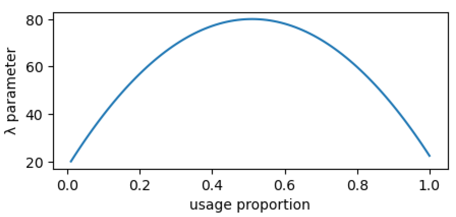
Another possible approach that already accounts for larger failure rates after longer periods of inactivity is to consider an MTBF dependent on the usage proportion. If a variable scale parameter $\lambda$ is chosen as in Figure 5 (with values ranging from 20 up to 80, depending on the usage proportion), the impact on availability would be as depicted in Figure 6, where some availability curves are shown for mean repair times between 10 and 50 (increments of 5).

It is clear that outermost usage proportions yield smaller availabilities. The best results are attained between $0.1$ and $0.2$, showing that too extreme a proportion is clearly a worst option.

2.2. Influence of Time to Failure Distribution

A complementary scenario to that of the prior subsection will now be appraised. To examine the influence on availability of failure distributions defined with different shape parameters, for the same mean repair time, the graphs that make up Figure 7 were drawn. Five random samples of failure data were obtained using Weibull distributions with shape parameters ranging from $k=1.5$ to $k=3.5$ ($0.5$ increments) and scale parameter $\lambda =40$. Random repair times were always generated by a Normal distribution with mean $\mu =10$ time units and standard deviation $\sigma =2$ time units, but the dynamics shown in Figure 7 are consistent across different mean repair times.

Again, the optimal operation regime was the 0%-100% standard; the same considerations already made in the previous subsection apply. Also, once more, the range of usage proportions from 0 to $0.1$ yielded just about the same availability—thus reinforcing the point made earlier about deviation from the 0%-100% regime.

Other noticeable aspects are related to the shape parameter of the failure distributions. For shape parameters closer to 1, there is a faster loss of availability over the entire range of usage proportions. For operation regimes close to $50\%$-$50\%$, the availability seems to be independent of the shape parameter.

3. Improving Availability of a Single Pump

In this section we will be looking into a sole pump of a hydropressor system (a “unary” system, so to speak), but now contemplating three possible failure modes—each with its own probability of occurring. Furthermore, this time around, preventive maintenance will also be included in the picture.

Usually, scheduled preventive interventions can be carried out with a smaller impact on overall downtime. As a matter of fact, the main cause for delays in repairs has to do with unexpected failures, which typically require the assembly of a maintenance crew (that may not be readily available), spare parts (that may not be in stock), to name just a couple. Once the unpredictability factor is removed from the scene, maintenance is conducted much more efficiently. Moreover, preventive maintenance can often be performed during periods where the equipment is mostly idle, thus lessening the impact of downtime even further. Under such assumptions, inherent availability is still a more than fair barometer of availability. Please note that this is quite unusual when considering preventive maintenance, for the notion of inherent availability expresses an intrinsic property of a device (the reason why just corrective maintenance is accounted for in its definition). It is only acceptable in this case in view of the particular circumstances at play.

Whereas in the prior section no discrimination among the types of failures was made, there will now be three possible ways for a breakdown to occur—not all equally frequent. One may think of this in more concrete terms by imagining three different (critical) components, say $C_i$ with $i\in \{1,2,3\}$, whose malfunction disables the pump; on top of that, it is known that upon a pump failure, there is a 50% probability of originating from $C_1$, a 30% chance from $C_2$, and 20% from $C_3$. There is also an underlying assumption in the discussion that a certain “risk level” has been accepted, meaning that an a priori probability p of corrective maintenance taking place (before it was supposed to) was agreed upon with the customer. For instance, $p=0.2$ means that the client is willing to countenance the possibility that, two times out of ten, corrective maintenance may be required ahead of time.

The issue to investigate is tied to the systematic preventive maintenance plan, which should be pursued to improve the pump’s availability. The results in the present section were obtained through the same principles described in the previous one. Random lifespans for the three components were sampled from Weibull distributions with the same shape parameter, $k=3.5$, and proportional scale parameters ${\lambda }_1=40$, ${\lambda }_2=40·{\displaystyle \frac{5}{3}}$, and ${\lambda }_3=40·{\displaystyle \frac{5}{2}}$ to reflect, respectively, the $50\%$, $30\%$, and $20\%$ chances of each type of failure occurring; for simplicity, and with minor loss of generality, the corrective maintenance repair times were taken to be constant, hence making the improvement in availability exactly equivalent to the improvement in average time between failures. A timespan of 100,000 time units was considered for each Monte Carlo trial, and a total of 100 trials were executed. As a first experience, a scenario of “total neglect” was attempted where no preventive maintenance was undertaken; in this case, we obtained an upper bound on the number of corrective interventions around 11,100, corresponding roughly to a mean time between failures of 18 time units.

3.1. Adding Preventive Maintenance

We began by taking a “greedy” approach to preventive maintenance, which basically amounted to carrying it out at every justifiable turn (so, a “total diligence” scenario). To put it more precisely: the strategy consists of performing a preventive intervention whenever $t_i^{\left(p\right)}$ time units have elapsed without a type i failure coming about – $t_i^{\left(p\right)}$ designates the probability p quantile of the $i\mathit{th}$ failure distribution.

This strategy is an extreme case aimed solely at establishing what sort of figures one gets with a maximal preventive maintenance policy (upon which we will then want to improve). The results are summarized in

Table 1. “Total neglect” vs. “total diligence” scenarios.

WITHOUT PREVENTIVE MAINTENANCE
Corrective interventions	11,100
Mean time between failures ($MTBF$)	18
WITH PREVENTIVE MAINTENANCE
Risk probability (p)	0.05	0.1	0.2
Preventive interventions	20,600	17,500	12,800
Corrective interventions	1100	2000	3300
Mean time between failures ($MTBF$)	170	97	60
Maximal attainable reduction (%)	49%	43%	31%

, for three different “risk levels” $p\in \{0.05,0.1,0.2\}$, where (unsurprisingly) the higher the risk one is ready to take, the less preventive maintenance weighs on the whole; values from the “total neglect” framework are included for comparison.

As can be seen, corrective maintenance is drastically reduced (by as much as 90%, in the case $p=0.05$), correlating with a glaring increase in the mean time between failures, but at the price of a huge percentage in maintenance now being preventive in nature (as high as 95%, in the case $p=0.05$). This is, of course, to be expected; the introduction of preventive maintenance curtails corrective maintenance, but increases the overall number of interventions. Obviously, a judgment on the trade-off should be subordinated to the relation between corrective and preventive maintenance costs. For instance, if $p=0.2$, for the reduction in corrective maintenance to pay off, the ratio of preventive maintenance cost to corrective maintenance cost should be lower than ${\displaystyle \frac{11,100-3300}{12,800}}\approx 0.61$; that is, roughly, a preventive intervention should cost less than 61% of a corrective one (and fairly so if solid financial gains are to be made).

To close the discussion, and with regard to the last row of values in Table 1, we note that an upper limit exists on how many interventions can be “spared” by a more polished preventive maintenance strategy. That is precisely what those percentages are signaling. Take the case $p=0.1$, for example; certainly, there can be no more than a

$${\displaystyle \frac{\mathrm{19,500}-\mathrm{11,100}}{\mathrm{19,500}}}\times 100\%\approx 43\%$$

reduction in overall maintenance, since the least number of interventions is achieved with the “total neglect” scenario. The last row of values then constitutes the best possible outcome in maintenance reduction, by means of preventive strategies, for each “risk level”.

We now make a brief comparison between the four scenarios, assuming the difference in cost between corrective and preventive interventions is known. Suppose the cost of a corrective intervention is equal to 3 and the cost of a preventive intervention is 1; then, by performing solely corrective interventions, the total cost would be 33,000, while with the parameters $p=0.05$, $p=0.1$, and $p=0.2$ it would become 23,900, 23,500, and 22,700, respectively, thus making $p=0.2$ the best option. If the cost ratio is 4 to 1 (or for even more unbalanced scenarios), the best option would be to consider $p=0.05$ with a total cost of 25,000. This points clearly in the direction of prioritizing preventive interventions, whenever their cost is significantly lower than that of corrective ones.

If material costs are taken into consideration, and since there is a quantifiable amount of average operating time wasted on a pump that was removed in a preventive intervention, we can compute the costs associated with these anticipatory interventions. In the case of very expensive materials being used, it may be better to accept greater risk (by increasing the value of p).

3.2. Refining Preventive Maintenance

In this subsection we improve upon the prior “greedy” approach to maintenance by lowering the number of preventive interventions on the basis of two cumulative strategies.

Since preventive maintenance will always make up a large share of general maintenance, it is desirable to try and find ways to mitigate its financial impact. For precisely this reason, one obvious course of action is to combine multiple preventive interventions (for the different components) into one single maintenance event. To make it clearer, say that two scheduled preventive interventions will have to be conducted in a short time frame. From both the financial and operational points of view, it could make perfect sense to perform them simultaneously by anticipating the later one (postponing the earlier one is surely unwise, since it increases the odds of a failure taking place in the meantime), thus doing away with one preventive maintenance instance altogether.

The previous example motivates the procedures that are described next, which depend on a prescribed time length T (to be set appropriately by a company). To clarify the first refinement made to the “greedy” strategy, let us suppose that we are on the verge of carrying out a preventive intervention. Then, we check if other ones are scheduled less than T time units away and, if so, all of these instances coalesce into a sole maintenance event. Naturally, a second refinement was then tried: to seize also corrective interventions for anticipating preventive ones—note that it is not feasible to do otherwise because, obviously, corrective interventions are (by nature) unexpected and cannot be scheduled.

Observe that, because $C_1$ fails more often than $C_2$, which in turn fails more frequently than $C_3$, for all $p\in ]0,1[$ one has

$$t_1^{\left(p\right)}<t_2^{\left(p\right)}<t_3^{\left(p\right)},$$

so that $t_1^{\left(p\right)}$ is a sort of minimal “threshold”, in the following sense: no preventive interventions related to the same component are scheduled less than $t_1^{\left(p\right)}$ time units apart. This fact imposes a natural constraint on the choice of the time length T, namely $T<t_1^{\left(p\right)}$, because multiple preventive interventions on the same component should not be allowed within the same timespan. As a consequence, there is a restriction on the number of interventions that can be combined: at most three, either all preventive in nature, or a corrective one and two preventive ones. The latter case includes the extreme situation of a failure in some component occurring just shy of scheduled preventive maintenance on all three components, the four events happening within T time units. Of course, under these circumstances, since a corrective intervention has to be performed, one of the preventive interventions just became redundant and will not be carried through.

The results on total maintenance reduction summarized in

Table 2. Reduction in maintenance with refined preventive maintenance strategies.

	Risk Probability (p)
Time Length (T)	0.05	0.1	0.2
1	5.4% ($+0.4\%$)	4.5% ($+0.6\%$)	2.9% ($+0.8\%$)
2	11% ($+0.5\%$)	8% ($+1\%$)	5% ($+1.5\%$)
3	14.7% ($+1.1\%$)	12.9 % ($+1.7\%$)	8% ($+2\%$)
4	18.5% ($+1.4\%$)	15.9% ($+2.2\%$)	10.6% ($+3.1\%$)
5	21% ($+1.5\%$)	18% ($+2.5\%$)	12% ($+3.8\%$)
6	22.3% ($+1.8\%$)	20% ($+3.3\%$)	14.4% ($+4.5\%$)
8	25.4% ($+2.5\%$)	22.6% ($+4.1\%$)	17.6% ($+5.8\%$)
10	—	24% ($+5\%$)	20% ($+7.5\%$)

are taken with respect to the “total diligence” framework of the previous subsection (you may want to recall Table 1). The percentages in parentheses are cumulative with the ones to their left and account for the additional gain made by also grabbing corrective maintenance instances to undertake preventive interventions.

To better grasp the results in Table 2, take (for example) the case $T=5$ and $p=0.2$. The table entry “12% ($+3.8\%$)” means that, regarding the same “risk level” in the “total diligence” scenario of the prior subsection, a 12% reduction in the overall number of interventions (16,100 for the case in question, according to Table 1) is accomplished by “fusing” preventive interventions, and an additional 3.8% by combining corrective interventions with preventive ones (yielding a total 15.8% reduction).

The computation of the percentage concerning the “meld” of preventive interventions is based on counting the number of occurrences in a timespan of T time units; yet, in the case of an intervention that could be “merged” with both a prior and an ensuing one, they would all have to be separated by less than T time units. This implies that, in order to use the reasoning that was followed to not double count the same “meld”, the value of $2T$ should be less than $t_1^{\left(p\right)}$. This is the reason behind the blank entry in Table 2: the case $T=10$ and $p=0.05$ was not simulated as it violates the above-stated constraint, because $t_1^{\left(0.05\right)}\approx 17$.

On a final note, observe also that by using larger time windows one gets more pronounced reductions in maintenance.

4. Conclusions

Although the parameters, with which the statistical distributions involved in the analysis were set, may not closely mirror actual observable values (notably the mean time to failure, or the mean time to repair), this does not detract from the general conclusions to which the results seem to point, as more accurate parameters would not yield a qualitatively different behavior.

Two scenarios were assessed: different mean times to repair were tested while the mean time to failure was kept fixed, and vice versa. In both scenarios a couple of salient features emerged:

• The numerically optimal solution was always the 0%-100% industry standard, the so-called “standby pump”/“duty pump” mode. However, in practice, there is a fair risk of system downtime due to long inactivity periods of the “standby pump” which, when needed upon failure of the “duty pump”, may well not start.
• For usage proportions (in one of the pumps) up to 10%, the differences in availability were negligible.

The latter suggests that if a minimal usage proportion can be set in that range, making the least used pump unlikely to fail on startup, the risk of system downtime can be virtually eliminated, with no apparent downside, if one “slightly” deviates from the 0%-100% configuration. It is worth noting that such a proportion will certainly vary with location, even for identical equipment, since the conditions (average temperature, humidity, etc.) under which they operate are bound to differ from place to place. This fact is usually not reflected in benchmark tests performed by manufacturers—which take place in nearly ideal operating conditions.

A distinctive hallmark of the approach, contrary to standard practice in industry, consists of allowing switches in the usage proportions of each pump after repairs. Numerical evidence that we provide shows that this simple procedure, in and of itself, already improves the system’s availability in a meaningful way.

The second challenge (Section 3) addressed the question of improving the availability of a single pump, admitting three failure modes that occur with different probabilities, and now adding also preventive maintenance to the mix. To better align with industry practices, where customers willingly accept some “risk level” (typically related to corrective maintenance (the most expensive one)), the analysis rests on the assumption that a maximal probability p of a corrective intervention to crop up is given from the outset. The associated time thresholds, $t_i^{\left(p\right)}$ with $i\in \{1,2,3\}$, below which the $i\mathit{th}$ failure type is expected to occur with $100p\%$ certainty, are given by the probability p quantiles of each failure distribution.

In a first approach to preventive maintenance, where the strategy amounted simply to performing a preventive intervention whenever a period of $t_i^{\left(p\right)}$ time units elapsed without a failure type i having occurred, a considerable reduction in corrective maintenance was already observed. This fact, needless to say, came at the expense of preventive maintenance weighing heavily on the whole (more so for lower values of p, predictably). Nevertheless, even with such a “crude” strategy, the trade-off might be desirable when the ratio of preventive maintenance costs to corrective maintenance costs is sufficiently favorable (and it can be)—potentially translating into noteworthy financial savings.

A refinement to the previous strategy was then made by “merging” preventive interventions which fell within a prescribed timespan (of T time units). Specifically, upon any preventive intervention related with a type i failure, say at some instant $t_i$, one seizes the occasion to check if more preventive interventions (linked to failure types $j\ne i$) are on the near horizon, that is, if instants $t_j>t_i$ exist such that $t_j-t_i<T$ (the value $t_k$ is a multiple of $t_k^{\left(p\right)}$); if so, those interventions are carried out simultaneously with the one currently underway. This course of action proved to have a non-negligible to somewhat considerable impact on the reduction of preventive interventions, more so for higher values of T and p. Although less pronounced, further reductions proved possible by likewise seizing instances of corrective maintenance as an opportunity to conduct preventive maintenance.