
Energy Efficient Access Point Placement for Distributed Massive MIMO
by
 , , , and
Yi-Hang Zhu
1,* ,
,
Gilles Callebaut
1,
Hatice Çalık
2,
Liesbet Van der Perre
1 and
François Rottenberg
1 1
ESAT-WaveCore, Ghent Technology Campus, KU Leuven, 9000 Ghent, Belgium
2
CODeS, Computer Science, Ghent Technology Campus, KU Leuven, 9000 Ghent, Belgium
*
Author to whom correspondence should be addressed.
Network 2022, 2(2), 288-310; https://doi.org/10.3390/network2020019
Submission received: 9 March 2022
/
Revised: 26 April 2022
/
Accepted: 5 May 2022
/
Published: 11 May 2022
Abstract
:Distributed massive multiple-input multiple-output (D-mMIMO) is one of the key candidate technologies for future wireless networks. A D-mMIMO system has multiple, geographically distributed, access points (APs) jointly serving its users. First of all, this paper reports on where to position these APs to minimize the overall transmit power in actual deployments. As a second contribution, we show that it is essential to take into account both the radiation pattern of the antenna array and the environment information when optimizing AP placement. Neglecting the radiation pattern and environment information, as generally assumed in the literature, can lead to a power penalty in the order of 15 and 20 , respectively. These results have been obtained by formulating the AP placement optimization problem as a combinatorial optimization problem, which can be solved with different approaches where different channel models are applied. The proposed graph-based channel model drastically lowers the computational time with respect to using an ray-tracing simulator (RTS) for channel evaluation. The performance of the graph-based approach is validated via the RTS, showing that it achieves 5 power saving on average compared with a Euclidean distance-based approach, which is the most commonly used approach in the literature.
1. Introduction
Distributed massive multiple-input multiple-output (D-mMIMO) is a technology that incorporates both the massive multiple-input multiple-output (MIMO) [1] and distributed antenna system [2] concepts. Due to the great potential regarding capacity and energy efficiency, D-mMIMO has been considered a promising technology for the future generations of wireless networks [3,4]. A D-mMIMO system deploys multiple access points (APs) that are connected to a central processing unit. By transforming the network from one central AP with a very large array to multiple APs at different locations, the average distance between the users to the nearest AP can be drastically reduced. Consequently, significant transmit power savings can be achieved. The channels of the users to the access infrastructure highly depend on the APs’ locations. Therefore, having a good AP placement is essential for exploiting the potential of the D-mMIMO system [5]. This paper aims to reduce the transmit power of the downlink by optimizing the AP placement. As an additional benefit, given the reciprocity in the setup, the optimized AP placement will reduce transmit power of the uplink as well.
When optimizing the AP placement, the environment information is an important parameter. It provides insight on two key aspects:
- (1)
- It includes information about the possible locations for deploying the APs.
- (2)
- It includes information regarding the objects, e.g., buildings, impacting the channel gain (the average signal power received at a given user when considering unit transmit power and including a potential antenna gain).
Regarding the first aspect, in practical scenarios, e.g., urban areas, APs are conveniently deployed on the walls along the streets or at the roofs’ edges. It is unlikely that APs are deployed, for example, in the middle of a street. The importance of the environment in this perspective may be less evident when the coverage region is large, e.g., 1 km by 1 km. In that case, modifying the generated AP placement by several meters to make the deployment feasible will have little impact on the system’s performance. However, in future wireless networks, the distance between APs and their users is going to shrink drastically due to the increasing AP density [6]. In this case, the system’s performance becomes very sensitive to the AP placement. Therefore, taking into account the environment information regarding any feasible locations for APs deployment is important. Nevertheless, most existing work is based on assumptions neglecting environment information [5,7,8,9,10,11,12,13,14,15,16,17,18,19,20,21,22,23,24,25,26,27,28]. In [7,10,11], the authors considered a distributed antenna system in a cell where all the transmitters and receivers are placed on a line. Another commonly used assumption is the circular topology [8,9,12,15,17,19,20]. It considers that the APs are placed evenly on a circle. This assumption was initially introduced to make the analysis of the optimization problem tractable [8]. It simplifies the problem to finding an optimal radius for the circle. A few earlier studies, e.g., [14,15,24,27], model the problem in a continuous way. They developed different gradient-based heuristic algorithms. Some other researchers applied Lloyd’s algorithm or k-means clustering-based approaches [11,18,21,25,28]. To the best of our knowledge, only [29,30] take into account the environment information. The focus of these studies, however, is on indoor and underground applications, respectively. This paper focuses on outdoor deployments and takes into account environment information about possible locations for deploying the APs.
Additionally, environment information regarding the possible AP locations is an essential prerequisite when considering the radiation pattern of the arrays. In the literature, the radiation pattern of the arrays in the APs is often ignored or assumed to be isotropic, which is not realistic: even the radiation pattern of antenna arrays with dipole elements is typically very directional in practice [31]. We have observed in our earlier work [5] that the radiation pattern has a significant impact on the optimal AP placement. To incorporate the radiation pattern, we need to take into account the broadside direction of the arrays at different locations, which critically depends on the environment of the AP locations. When deploying an AP on a wall, the AP can be installed in a less visible way [32] and catch less wind, for aesthetics and deployment simplicity. The broadside direction of the array will be perpendicular to the wall and towards the street. In this paper, we consider different antenna types for the array and we deploy the APs on the walls of buildings.
For the second aspect, the obstacles in the environment, e.g., buildings, have a significant impact on the channels. The channel models applied in the current literature for optimizing the AP placement take a limited amount of environment information into account [8,9,10,11,12,13,14,15,16,17,18,19,20,21,22,23,24,25,26,27,28]. Specifically, large-scale fading is usually modeled based on certain statistical distributions and the Euclidean distance between user locations and APs. Those models work well for the traditional cellular systems where the coverage region is large. In that case, the propagation distance between a base station and a user location is large and can be well approximated by a statistical distribution parametrized by the Euclidean distance. However, as coverage regions become small, the discrepancy between the propagation distance and Euclidean distance becomes significant, and empirical propagation conditions are highly location-specific. Therefore, those statistical models are no longer appropriate.
As suggested by [33], a propagation model which is based on real-world geographic information is indispensable for realistic optimization of the AP placement. In [33], the authors model the propagation environment using a ray-tracing simulator (RTS) together with an iterative procedure for the AP placement optimization. An RTS considers multipath radio propagation as rays, taking into account different radio propagation mechanisms, namely reflection, scattering, and diffraction [34]. Therefore, an RTS is able to accurately simulate the channel gain considering the impact from the environment. However, using an RTS for channel evaluation is computationally intensive [34], especially if this has to be done for many potential AP locations and mobile users that may be anywhere in the coverage zone. Therefore, it is not scalable to apply an RTS for the AP placement optimization. The impact of buildings on the channel gain is also considered by [35,36] where different pathloss exponent values for different scenarios together with the Euclidean distance are utilized. However, estimating the pathloss exponent values for a large number of scenarios is a cumbersome task. In this paper, we introduce a graph-based approach to effectively capture environment information. Given that planning the AP placement is a strategic level decision, elements in the environment that move or change within short time intervals, e.g., cars, are not considered.
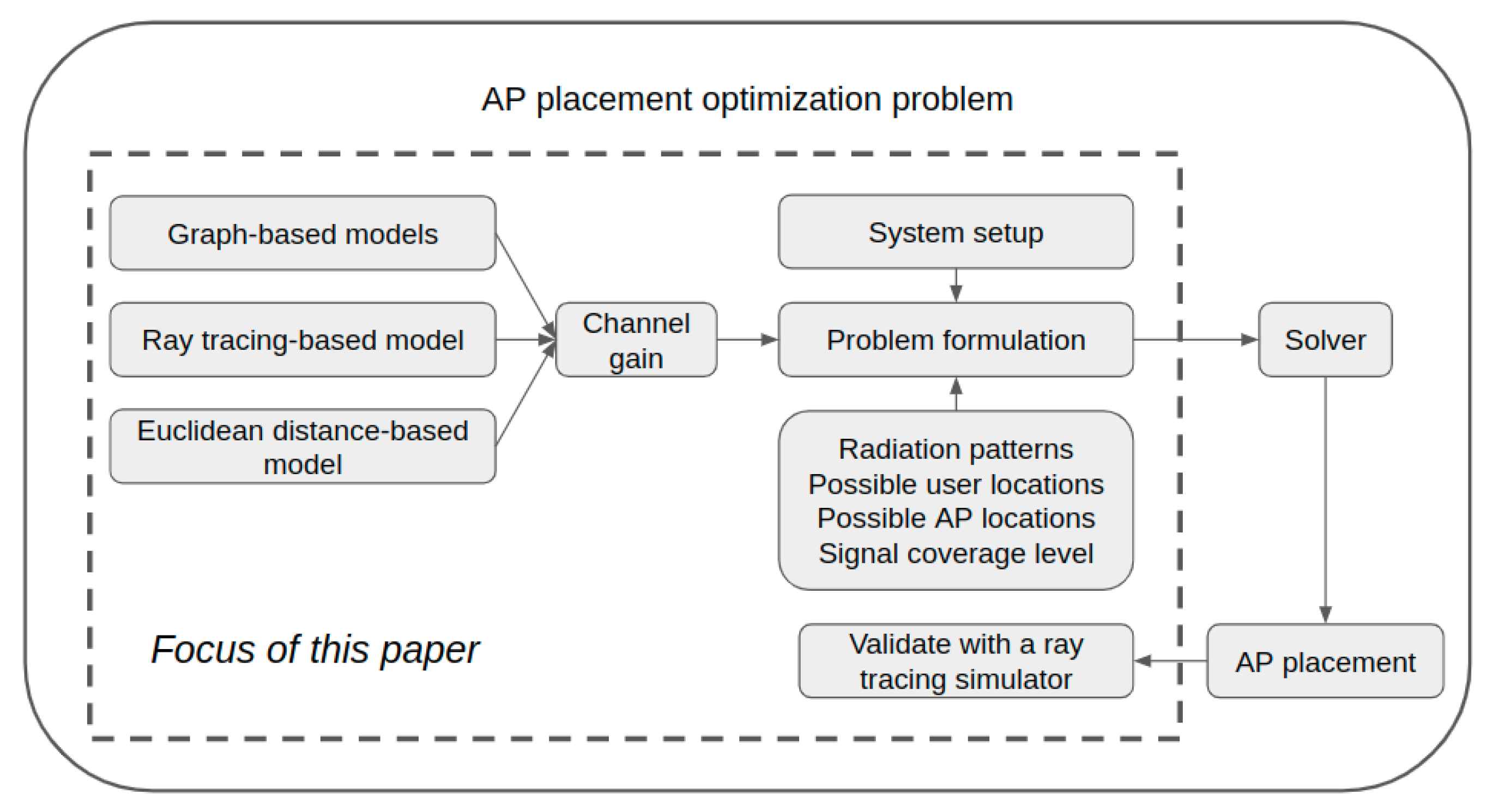
As illustrated in Figure 1, this study focuses on the modeling part of the AP placement optimization problem.
The contributions of this paper are as follows:
- We propose a graph-based approach for modeling the physical propagation. The approach effectively captures the obstacles in the environment and radiation pattern of the arrays, taking into account the possible broadside direction of the arrays at different potential AP locations.
- Based on an RTS, provided by Huawei Technologies (Gothenburg, Sweden), we perform a numerical validation of the graph-based approach and the channel models that have been introduced in the literature, considering different signal coverage levels and antenna types. We demonstrate that it is essential to take into account the radiation pattern of the arrays and environment information regarding the possible user locations, AP locations, and radio wave propagation.
The rest of the paper is structured as follows. Section 2 details the considered D-mMIMO system and formally describes the problem. Section 3 presents different ways to model the channel gain, including our proposed graph-based approach as well as others mentioned in the literature. Section 4 discusses the simulation results and Section 5 concludes the paper.
Notation: An upper case letter in the default math font, e.g., V, represents a constant. An upper case letter in mathcal font, e.g., , is a set. Indices are denoted only using subscripts in lower case, e.g., l in . Vectors are denoted by lower case letters in bold, e.g., . The complex conjugate is denoted as . The 2-norm of a vector is denoted as . The integer part of a value is denoted by . The total number of elements in a set, e.g., , is denoted as . The imaginary unit, , is represented by , and statistical expectation is denoted by .
2. System Model and Problem Formulation
Figure 2 illustrates an example of an area that needs to be covered by the D-mMIMO system to be deployed.
2.1. System Setup
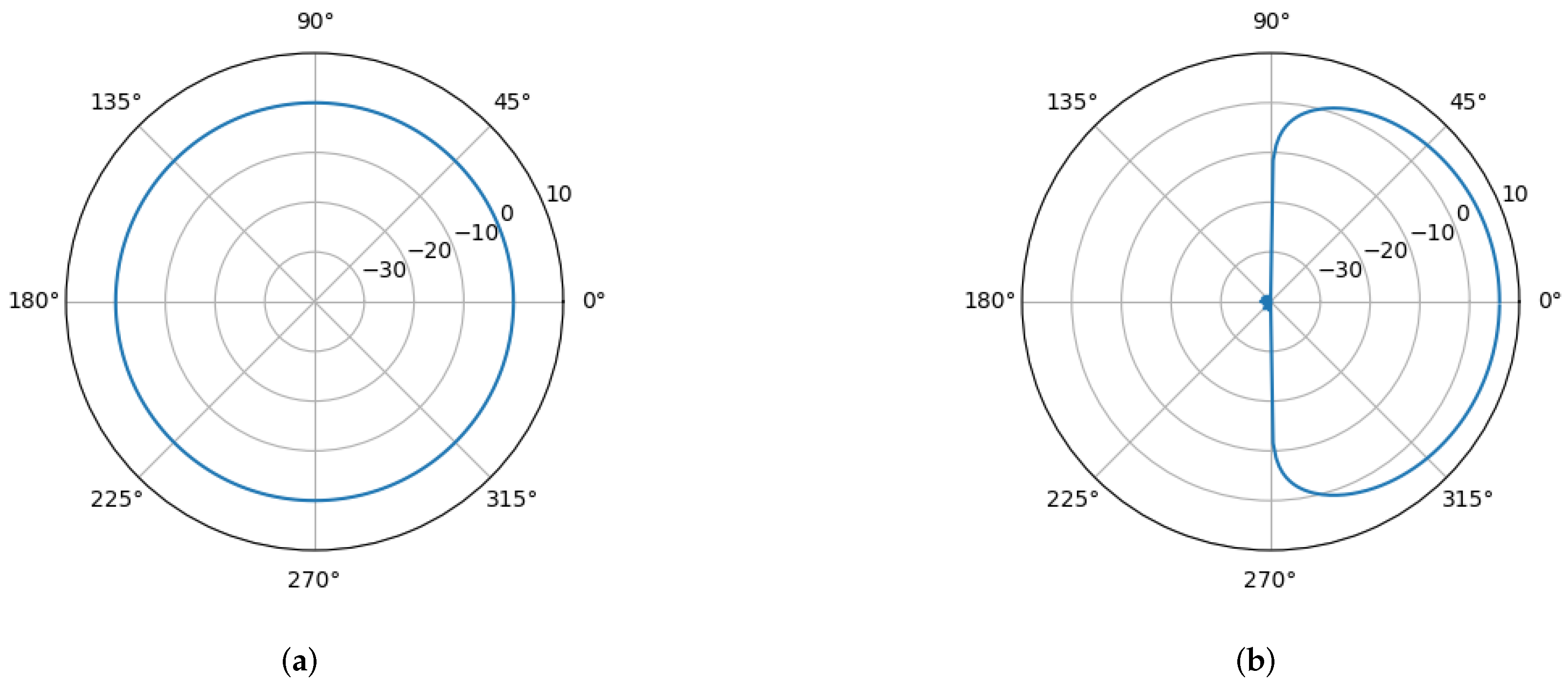
The number of APs in the D-mMIMO system is equal to T. These APs are used to jointly serve each user in the coverage region. Each AP has a half wavelength-spaced antenna array, hosting M elements. Two types of antenna elements are considered: patch antennas and isotropic antennas. The radiation patterns for the two types of elements are illustrated in Figure 3.
2.2. Potential User Locations
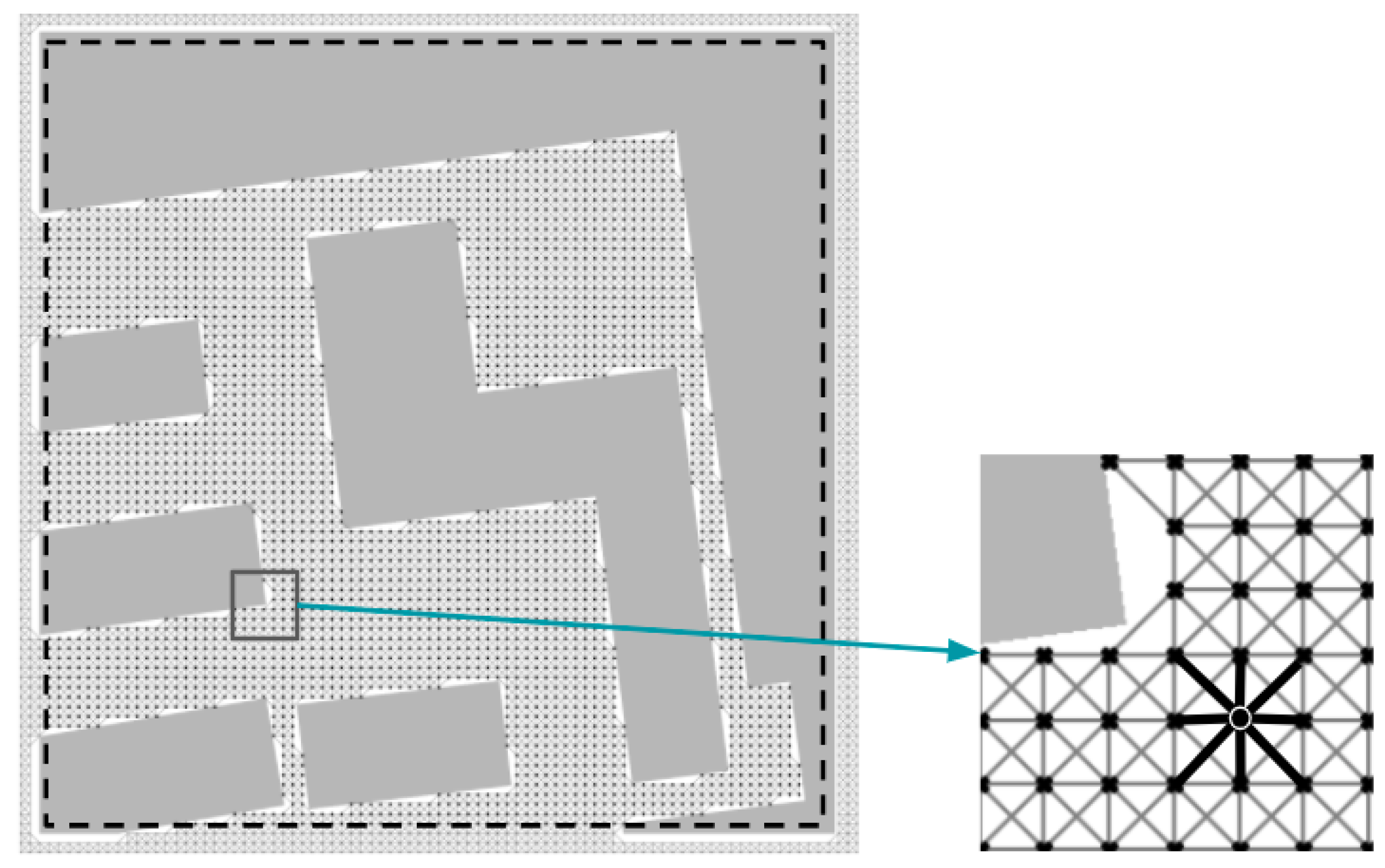
Each user is equipped with a single isotropic antenna. The black dots in Figure 2 illustrate the users’ possible outdoor locations. These locations are initially generated in a way that they are one meter apart from each other and uniformly cover the region. The points that are encapsulated by buildings are then excluded from the set of all considered user locations in the region, which is denoted as .
2.3. Potential AP Locations
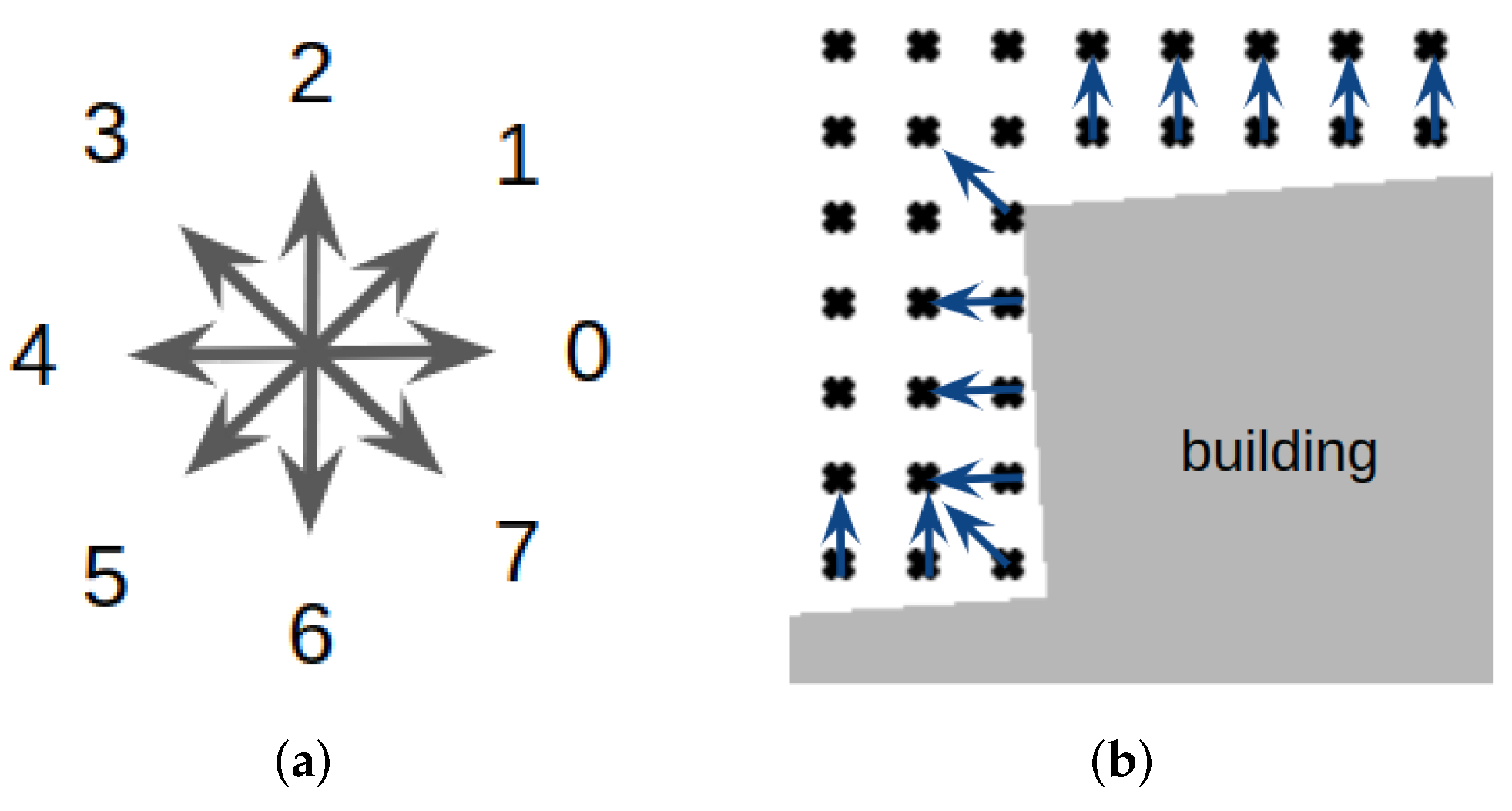
The user locations next to a building are also potential locations for deploying the APs of the D-mMIMO. The set of all potential AP locations in the region is denoted as . When installing an AP at a given location, we assume that the AP is installed vertically. The broadside of the AP’s array is set with respect to the location. For simplicity, we consider eight possible broadside directions, as illustrated in Figure 4a. The direction for mounting an AP in each potential location is selected in a way that the broadside is perpendicular to the building as much as possible, as illustrated in Figure 4b.
2.4. Signal Power at Each Potential User Location
As mentioned earlier, the decision on the AP placement happens at a strategic level. It involves a lot of uncertainty. Therefore, the impact of imperfect channel state information is not considered. To simplify the calculation of the average received signal power, we assume the availability of perfect channel state information and maximum ratio precoding, thereby ensuring that the signals from the APs coherently combine at user locations. When simultaneously sending signals from distributed APs, the received signal at location i is calculated as
where the binary variable equals one if an AP is deployed at a location l and zero otherwise. We denote the channel response between a user location i and an antenna element m in the array of AP l as . The information signal s is precoded by applying the precoding weight
which determines the spatial directivity of the transmission. The additive white Gaussian noise has zero mean and variance .
The transmit power in the information signal equals the total transmit power in the system . The average received signal power at a user location i is defined as
We denote the average channel gain between an AP l and a location i by and compute it as
The average received signal power can then be expressed as
Different ways of modeling are discussed in Section 3.
2.5. Mathematical Formulation
We aim to reduce the transmit power by optimizing the AP locations, while providing the desired signal coverage in terms of minimum average received signal power at all potential user locations. In other words, we target to use the minimal amount of transmit power while ensuring that the users receive sufficient signal power wherever they are within the covered region. In order to formulate the AP placement optimization problem, we define the following decision variables: the transmit power per AP ; if an AP is deployed at a location l, otherwise ; if a user location i is covered with sufficient signal, otherwise. In addition to the aforementioned parameters, we define to denote the minimum required average received signal power at each user location and to denote the signal coverage level in percentage ( corresponds to zero signal coverage and corresponds to full signal coverage). The AP placement optimization problem can then be formulated as Equations (6)–(9). The notation utilized for the formulation is given in Table 1.
Objective function (6) minimizes the transmit power per AP. Constraint (7) guarantees that T locations are selected for AP deployment. Constraints (8) ensure that the average received signal power at a covered user location is not lower than the minimum required amount . Constraint (9) ensures the desired signal coverage level.
3. Different Channel Models
This section discusses three different ways of modeling the average channel gain () between AP location l and user location i. Section 3.1 discusses a model that is based on the Euclidean distance between the locations. Section 3.2 introduces our proposed graph-based approach for modeling the channel gain. Section 3.3 calculates the channel gain based on channels that have been simulated with an RTS.
3.1. Euclidean Distance-Based Model
Let us denote the channel gain from AP location l to user location i as . Considering the generic statistical model commonly applied in existing studies [14,39] and the radiation pattern of the array in the AP (the user has a single isotropic antenna), we calculate as
where is the angle of user location i regarding the broadside direction of the array at AP location l and is the antenna gain from the AP at location l in the direction of user location i. Parameter is the free space loss factor [40] determined by the wavelength. The power loss due to the propagation distance is represented by , where two is the pathloss exponent and is the Euclidean distance between user location i and AP location l. We model the shadowing as , where is a zero mean Gaussian random variable with a given variance. Each entry of the small-fading vector is an independent and identically distributed Gaussian random variable with zero mean and unit variance. Considering Equation (10), the average channel gain is defined as
The distributions of shadowing and small-scale fading in the model are commonly assumed to be independent of AP location l and user location i [14]. The constant is also independent of the user location and the AP location. Therefore, we can state that the constant equals
and reformulate Equation (11) as
Regarding Constraints (8), the value for has no impact on the optimal AP placement. This is consistent with the conclusion made in [14]. We only use Equation (13) for calculating the AP placement and then evaluate the required transmit power with an RTS. Therefore, we simply set to one in our experiments.
As indicated by Equation (13), the average channel gain received at a user location i from an AP location l is only characterized by the Euclidean distance between both locations. As such, it does not consider the local environment information, for example buildings, causing obstruction or not. Consequently, the estimated may not correspond to the direction of the highest power. This is illustrated in Figure 5, using the same map as in Figure 2. The two highlighted dots in Figure 5 represent a user location and an AP location. The blue arrow represents the broadside direction of the array at the AP location. The green straight line indicates the Euclidean distance between the user location and the AP location. The orange polyline in Figure 5 illustrates one of the possible propagation paths from the AP location to the user location. As shown in Figure 5, the Euclidean distance-based model ignores the building between the user location and the AP location. For both the angle of departure and length, the green line significantly deviates from the orange polyline. The channel gain may be severely overestimated if we estimate it based on the green line.
3.2. Graph-Based Models
Motivated by the limitations of the Euclidean distance-based channel model, we introduce a novel way of modeling the channel gain based on a graph. The rationale behind is as follows: When sending a signal from an AP to a location, the user at that location will receive the signal from different directions, which are referred to as multipath components. Among them, there may be one or two dominant ones, which can be approximated based on a non-obstructed path from the AP location to the user location. Based on this reasoning, we introduce a graph-based approach for modeling the channel gain. Instead of using the Euclidean distance , we consider a value , which is computed based on a path between a user location i and an AP location l. Given that the angle for the antenna gain also depends on the propagation paths, we directly incorporate the antenna gain into . For the graph-based models introduced in this section, we define the average channel gain as
The details of the methods for finding the shortest paths to be utilized in calculating are presented in Section 3.2.2. Before going into these details, we first introduce a graph-based model for the environment.
3.2.1. A Graph for Capturing the Environment
Figure 6 illustrates an example of the graph that we use to capture the environment in a given map. The nodes in the graph are one meter apart and directly connected to their neighbor nodes via edges. Each node within the coverage region, the dashed line in Figure 6, is associated with a generated location mentioned in Section 2. Due to the grid structure, each node is associated with at most eight edges.
Utilizing this graph, we aim to approximate the average channel gain based on a non-obstructed path from the AP locations to user locations. We determine the value of parameter by computing all the best found paths between each location and location . The procedure for computing the paths is presented in the next section.
3.2.2. Algorithm for Searching Paths
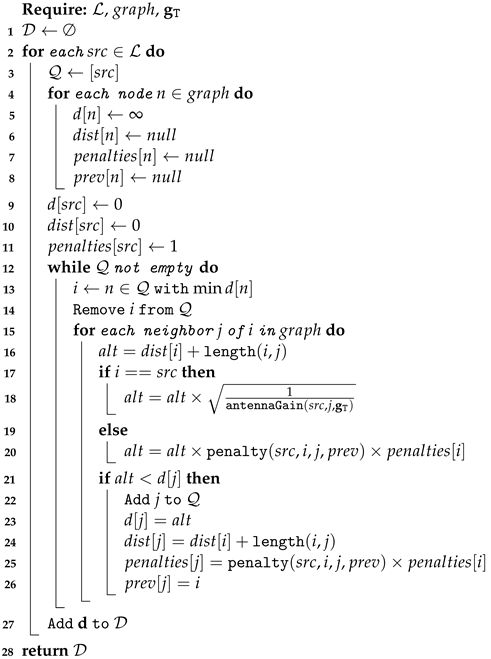
The shortest path problem is well known, and many efficient algorithms are available in the literature for solving this problem, e.g., Dijkstra’s algorithm [41], A* search algorithm [42] and Floyd–Warshall algorithm [43]. Due to the nature of the graph and the paths that we need to search for, we base our implementation on Dijkstra’s algorithm [41]. Algorithm A1 in Appendix A presents the pseudocode of our pathfinding method. Algorithm A1 includes two sub-procedures: Algorithms A2 and A3. The pseudocode and further details of these algorithms are provided in Appendix A as well. We use Algorithm A1 to search for a path from each AP location to location that gives the lowest value for . Our hypothesis behind the algorithm is that when sending a radio wave from a location l to a location i, the propagation path loss during will increase with (1) increased propagation distance between the two locations, (2) reflections, scattering and diffraction due to obstacles, and (3) when there is a mismatch between the angle of departure and the broadside direction of the AP at location l. We try to incorporate these three effects into parameter . A smaller corresponds with a higher average received signal power at location i.
3.2.3. Two Graph-Based Models
Based on Algorithm A1, two models are introduced.
- Shortest path-based model: this model does not consider the pathloss due to angular changes. Hence, in Algorithm A1 is fixed to one.
- Angular penalty-based model: this model takes into account the pathloss, e.g., due to diffraction. Hence, is calculated via Algorithm A3.
3.3. RTS-Based Model
The Euclidean distance-based model and the two graph-based models can compute the average channel gain in seconds. However, those models cannot accurately capture information about the environment. The average channel gain computed via those models is an approximation of the real one. Given that an RTS is able to accurately capture environment information [34], this section introduces an RTS-based approach. The RTS is provided by Huawei Technologies (Gothenburg, Sweden). We use the approach to evaluate the solutions generated by the other, less complex, channel models. The RTS considers a set of evenly spaced sub-carrier frequencies within a given bandwidth. The average channel gain for the RTS-based model is computed as
where is the channel response between user location i and antenna m of the array of the AP at location l when frequency f is used. Set includes all the sub-carrier frequencies within the considered bandwidth. As mentioned in Section 1, the RTS-based model is computationally intensive. In Section 4, two methods are applied to simplify the computation.
4. Simulation Results
In this section, six questions are investigated:
- Q1:
- Where are the user locations that have a high impact on the total transmit power?
- Q2:
- With the optimized AP placement, what is the relation between the total number of APs and the performance of the D-mMIMO system?
- Q3:
- Is it important to take the radiation pattern of the arrays into account when optimizing the AP placement?
- Q4:
- Is it essential to take more environment information into account when optimizing the AP placement?
- Q5:
- Does the angular penalty-based model perform better than the Euclidean distance-based model?
Our analysis considers five distinctive maps, maps 1–5, which are discussed in Section 4.1, and two scenarios with different antenna elements.
- Scenario I:
- isotropic antennas are used in each AP.
- Scenario II:
- patch antennas are used in each AP.
For each scenario, 11 signal coverage levels are considered. The parameter setup is summarized in Table 2.
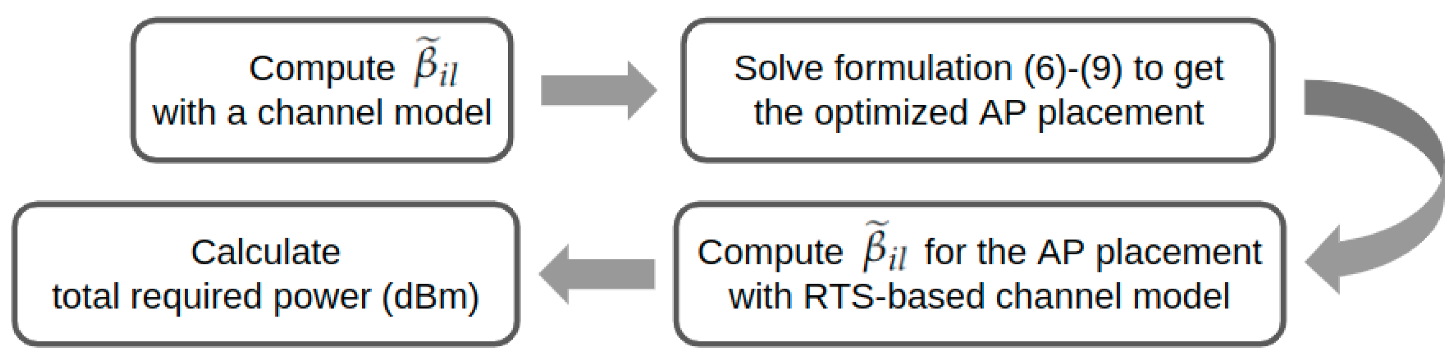
Figure 7 illustrates the procedure for executing the experiments. For a given channel model, we first use it to generate the average channel gain via Equations (11), (14) or (15). Then the optimal AP placement is generated by solving Formulations (6)–(9) with the generated . Noticeably, we always optimally solve Formulations (6)–(9) regarding the considered solutions space, the set of potential AP locations. In this way, we eliminate the impact of the efficiency of the solver on the results. The approach that is used to solve the formulation is detailed in Section 4.2. For each generated optimal AP placement, except the ones generated via the RTS-based channel model, we use the RTS-based model to compute the channels, which are regarded as the ground truth. Then the total transmit power () for the AP placement is calculated based on the channels generated via the RTS-based model. The experiments are executed on a machine with 20 Intel Xeon(R)W-2155 CPU @ 3.30 GHz processors, one NVIDIA Quadro P6000 GPU, and Windows Server 2016 system.
4.1. Reducing Potential User Locations
The generated user locations are one meter apart, as mentioned in Section 2. The total number of the generated user locations is large. Considering a 100 by 100 coverage region, for example, the total number of the user locations within the coverage region is more than 5000, which results in a long computational time when running the RTS to validate the AP placements. This motivates us to find a way of reducing the total number of user locations.
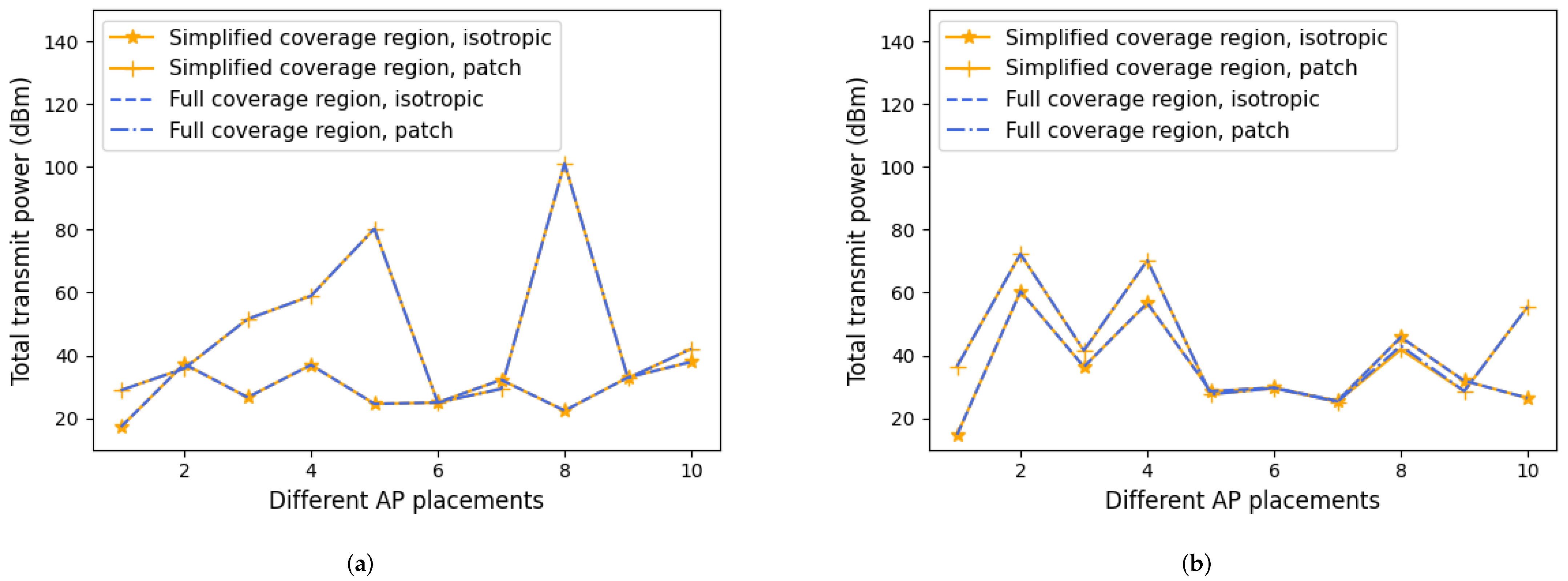
We hypothesize that, for a given user location that is fully surrounded by eight user locations, the user location will surely receive sufficient power if the other eight locations have received sufficient power. This implies that we only need to consider the signal coverage for locations that are not fully surrounded by other locations. The user locations, which are either next to a building or on a boundary of the considered coverage region, are the essential user locations. To test this hypothesis, we calculate the total required transmit power via the RTS-based model using a four-ap D-mMIMO system for 10 randomly generated AP placements. Two antenna types and two maps are considered. The targeted signal coverage level is 100%.
The result of this simulation is illustrated in Figure 8, where a full coverage region means that all the user locations are included, while a simplified coverage region only includes essential user locations. Figure 9 gives an example for the heatmaps of the average received signal power in dBm at each location when considering an AP placement on map 1. The red spots in Figure 9 represent the APs, and the orange spot indicates the user location that receives the overall lowest power. The results in Figure 8 and Figure 9 confirm that the total transmit power and the user location that receives the overall lowest power for each AP placement remain very similar when we consider a full coverage region or simplified coverage region. This implies that most of the essential locations have been included in the simplified coverage regions.
The required computational time is given in Table 3, demonstrating that the simplified coverage region results in a 4 to 8 times lower computational time compared to the full one. Therefore, we use the simplified coverage regions approach in RTS experiments and when solving Formulations (6)–(9).
Figure 10 illustrates the simplified coverage regions for the five maps, generated as follows. The data of a selected region is exported from OpenStreetMap. The RTS is used to generate the coverage region, adding 2 ’s padding around each map for easier processing of the buildings on the map. Then we keep 3 ’s margin between the borders of the map and the coverage region.
4.2. Reducing Potential AP Locations
We aim to find the optimal AP placement with the RTS as a benchmark to evaluate the solutions obtained by using the other channels models. Therefore, we evaluate all the channels for each potential AP location. However, the RTS still requires around 400 to simulate the channels for each potential AP location, resulting in several days to compute the channels for all the potential AP locations in one coverage region. Therefore, we reduce the total number of analyzed AP locations to 100 by selecting one location every locations. Hence, the set of the 100 selected locations, denoted by , has a similar distribution as the AP locations in . We further also use the in Formulation (6)–(9), which allows us to enumerate all the possible solutions in around one minute. Therefore, we simply solve the problem by the enumeration procedure instead of a more sophisticated solver.
Noticeably, the reason for reducing the potential AP locations is because the RTS is computationally not scalable. The latter does not apply to the novel approaches presented in this paper.
4.3. Analysis with Perfect Environment Information
In this section, we investigate Q2 and Q3, which are related to the total number of APs in the D-mMIMO system and the radiation pattern. We do the analysis using the RTS-based model instead of the other models for the AP placement optimization. In this way, we eliminate the impact of imperfect environment information on the results. The relevance of environment information regarding the channel gain is further analyzed in Section 4.4.
4.3.1. Impact of the Number of APs in the D-mMIMO
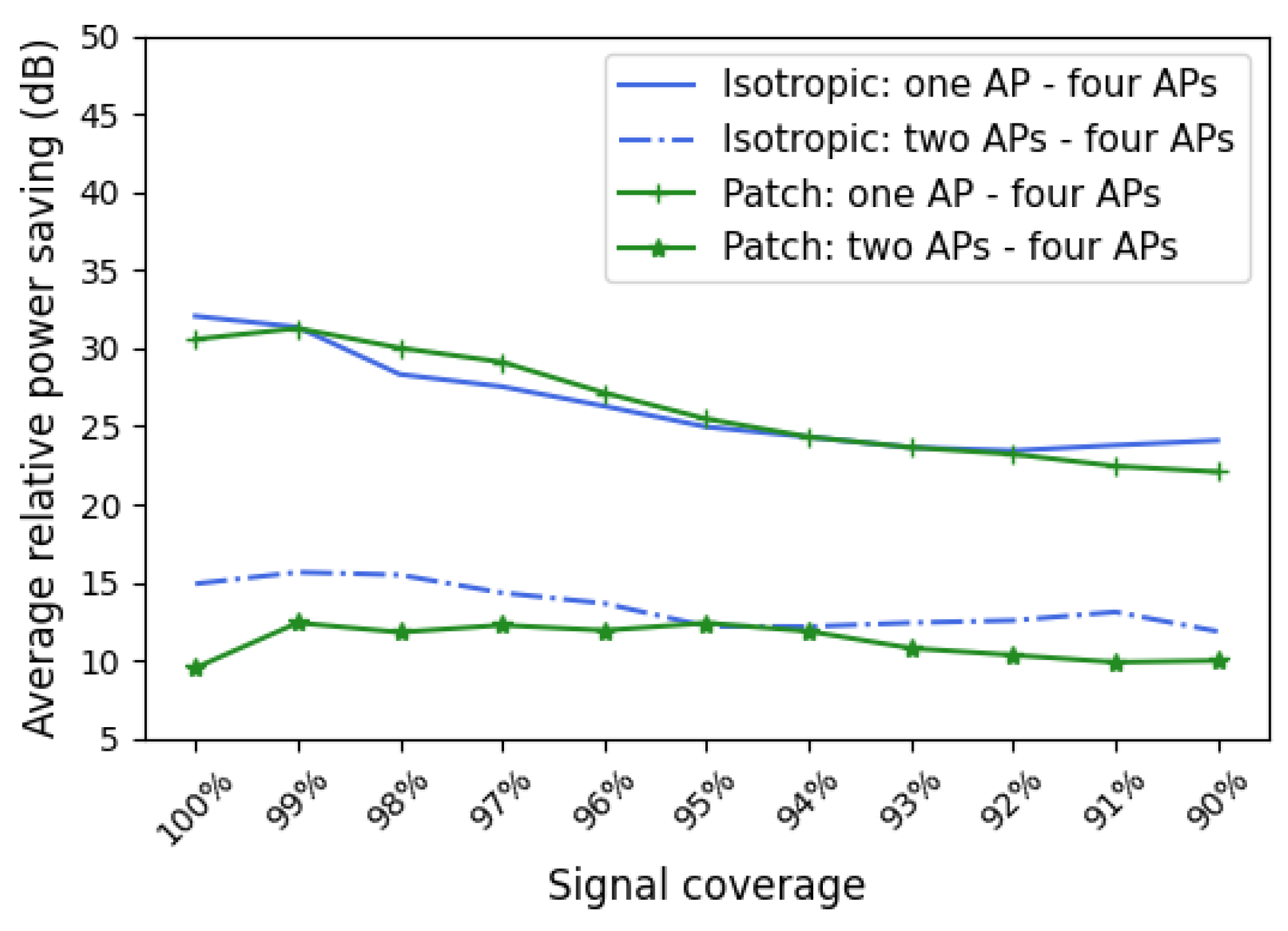
We consider a D-mMIMO system with 128 antennas in total (see Table 2). We assume that each AP has the same number of antennas. This section investigates the question of how to decide on the number of APs in the system. We generate optimal placements via the RTS-based model for three cases: (a) four APs, (b) two APs, and (c) one AP.
The average relative power saving between different configurations over all the maps is illustrated in Figure 11. For example, the full blue line in Figure 11 represents the average relative power saving of using the system with four APs compared with the system with one AP, using isotropic antennas. The results show that the total number of APs has a huge impact on the system’s performance. The system achieves the best performance when it has four APs. On average, it saves around 22–32 transmit power compared with the one-AP system and 9–15 power compared with the two-AP system. In future research, it may be interesting to study potential further enhancements by deploying more APs.
4.3.2. Value of Radiation Pattern Information
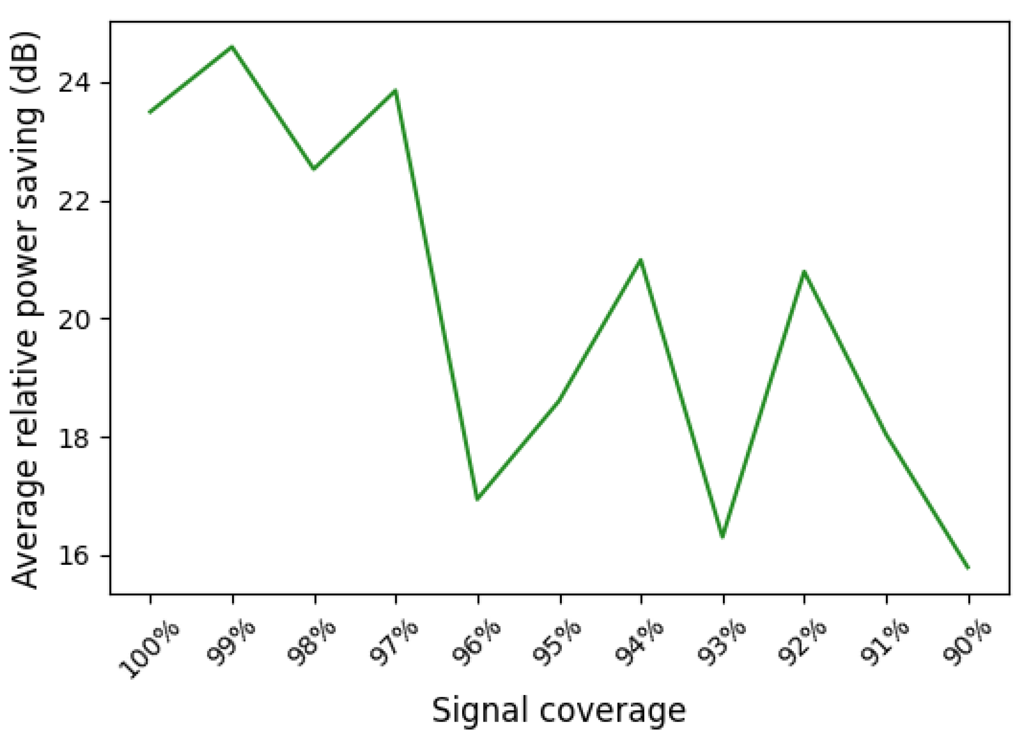
In most of the current literature on optimizing the AP placement, the radiation pattern of the arrays is assumed to be isotropic, which is, however, unrealistic. This section analyses how power savings are impacted by taking the radiation pattern into consideration. We consider a D-mMIMO system with four 32-element APs. All antenna elements are patch antennas. Two sets of AP placements are generated for each of the five maps. The solutions in set 1 are generated without considering the radiation pattern, while set 2 takes into account the patch antennas. The solutions in set 2 and set 1 are compared in Figure 12, demonstrating an average power saving ranging from 15 to 24 . This confirms the significance of taking into account the radiation pattern of the antennas, consistent with [5].
As mentioned in Section 1 considering environment information regarding the potential AP locations is a preposition of considering the radiation pattern. Therefore, the results also imply that it is essential to consider environment information for the AP placement optimization problem.
4.4. Different Channel Models
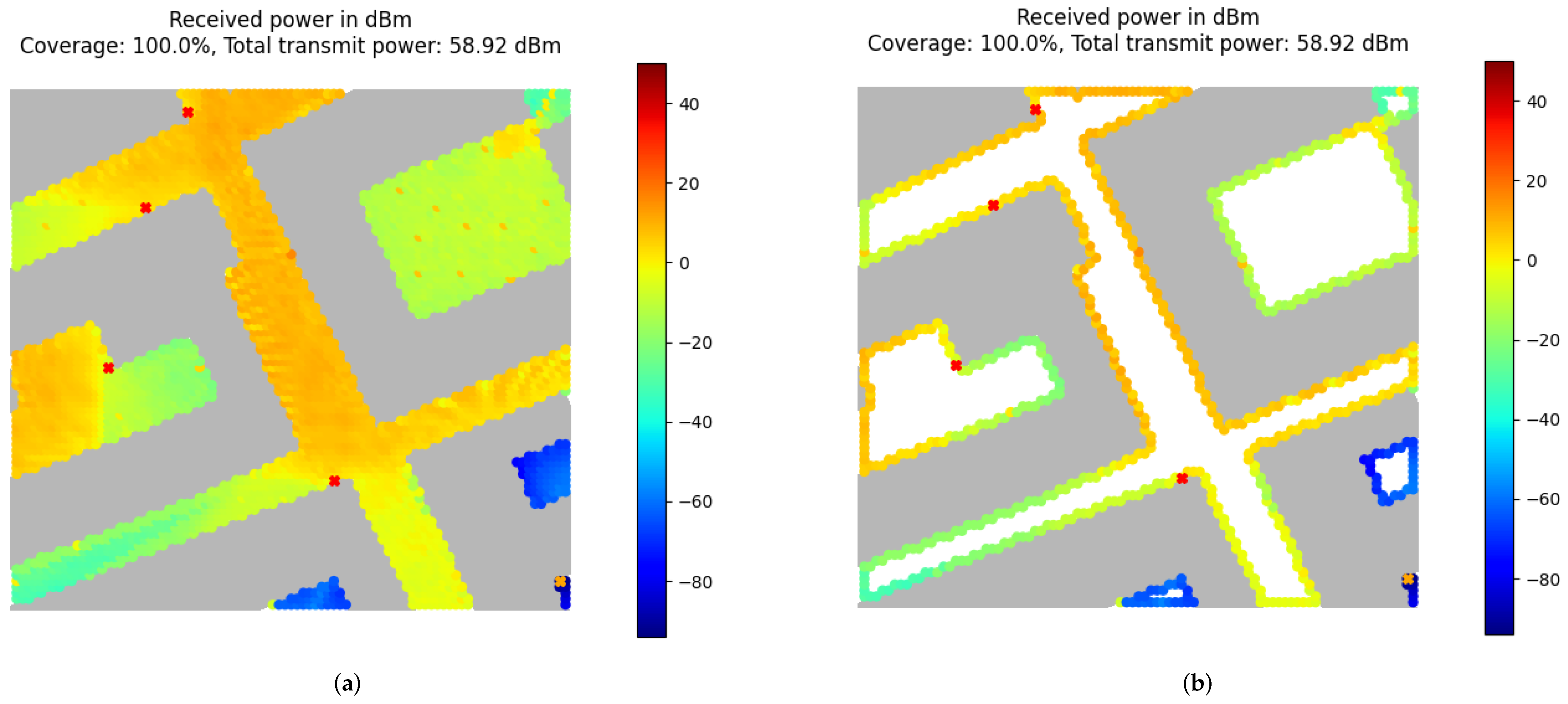
This section assesses Q4 and Q5. We analyze the value of environment information regarding channel gain for the AP placement optimization. We also compare our proposed channel models with the Euclidean distance-based model, which is commonly used in the literature. We consider a four-AP D-mMIMO system and four channel models discussed in Section 3. The heatmaps for the received power simulated via the RTS when using the AP placement generated by the different channel models for map 5 are illustrated in Figure 13. The heatmaps suggest that the Euclidean distance-based model, which represents the commonly applied model in the literature, generates a low-quality AP placement compared with the other models. The main reason here is that the Euclidean distance-based model ignores the building blocks when estimating the angle of departure for the arrays. Figure 13 demonstrates that environment information is very important when considering the radiation pattern of the arrays.
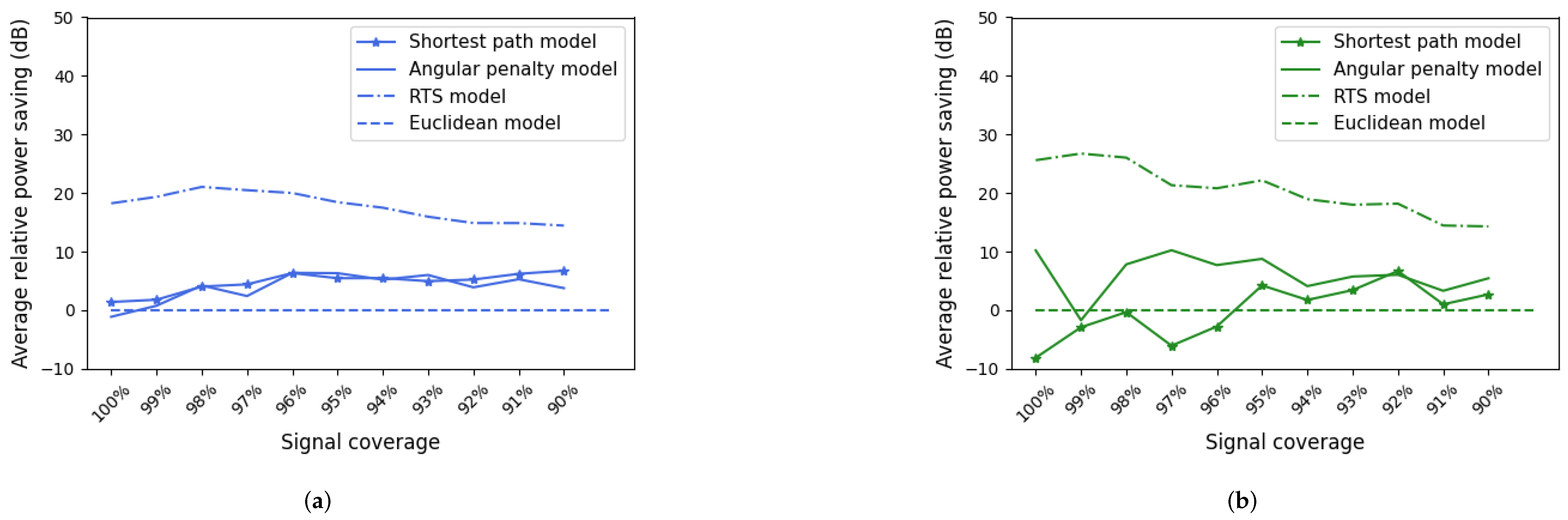
The average relative power saving when using the shortest path-based model, angular penalty-based model, and the RTS-based model compared with the Euclidean distance-based model over all the maps is illustrated in Figure 14. The result in Figure 14a, for example, corresponds to the scenario where we use isotropic antennas.
In general, the power saving in Figure 14 is higher when using patch antennas instead of isotropic antennas. This is consistent with the results in Figure 13. Additionally, Figure 14 indicates that the setup generated via the RTS-based model requires the least power compared with the setups found with other models (for all the scenarios). It saves around 20 compared with the Euclidean distance-based model. This is expected given that the RTS-based model is regarded as the ground truth in this paper. It accurately captures environment information. The results further confirm the importance of considering environment information regarding channel gain for the AP placement optimization.
As mentioned in Table 3, the RTS-based model requires around 1000–2000 s to evaluate all the channels for each AP placement in a simplified coverage region. Table 4 lists the average time that is required for different channel models to evaluate the channels for all the possible AP placements in a simplified coverage region. As shown in Table 4, the RTS-based model requires very long computational time. Therefore, it is interesting to consider the other models for the AP placement optimization. The two graph-based models: the shortest path-based model and the angular penalty-based model are proposed in this work. These models take around one minute to generate the average channel gain for all the possible AP locations. As suggested by Figure 14, using the AP placements generated via the two graph-based models, particularly, the angular penalty-based model, power saving is achieved compared with the Euclidean distance-based model in most situations. The average relative power saving of using the angular penalty-based model is around 5 compared with the Euclidean distance-based model. This is consistent with the fact that the two graph-based models contain more environment information than the Euclidean distance-based model. The results in Figure 14 also suggest that, in general, the angular penalty-based model performs better than the shortest path-based model. This implies that it is important to take the pathloss due to scattering into account when optimizing the AP placement.
Moreover, Figure 14 indicates that the average relative power saving is correlated with the coverage level. The reason is that the required power at a coverage level is determined by the location which receives the lowest power among all the covered locations. The location is more sensitive to the local environment when the coverage level is high. So, it requires a channel model to include more local environment information to accurately find the particular location when the coverage level is high. This explains why the performance of the Euclidean distance-based model and the two graph-based models is dependent on the coverage level.
5. Conclusions
In this paper, we focus on reducing the transmit power of a D-mMIMO system by optimizing the AP placement. Although we have only considered the downlink, given the reciprocity between downlink and uplink, the optimized AP placement will also relax transmit power requirements for the users. We formulate the AP placement problem as a combinatorial optimization problem. A simplified coverage region is applied, which results in significantly less computational time while having little impact on the solutions. With this approach, we have analyzed the performance of the D-mMIMO using an RTS-based model for optimizing the AP placement. Different antenna types and signal coverage levels are considered. Our results have demonstrated the significance of environment information, feasible locations for deploying APs and radiation patterns, which are commonly neglected in the existing studies. The consideration of the radiation pattern leads to a power saving of around 15–24 dB. Furthermore, using four APs instead of one or two APs in the system brings a power saving of more than 22 and 9 , respectively. Additionally, a power saving of around 20 is achieved by evaluating the channels with perfect environment information. The RTS-based model precisely captures environment information and generates a very good AP placement, however, it is computationally intensive and not scalable. For this reason, we have introduced a graph-based approach to effectively approximate the channel gain. The performance of this approach has been evaluated via the RTS. The results show that the graph-based approach saves around 5 power compared with the Euclidean distance-based approach, which represents the commonly applied model in the literature.
Nevertheless, this work has some limitations which can be addressed in future work. The gap between the transmit power when using the graph-based approach and using the RTS-based model is still large. Therefore, the graph-based approach requires further improvement. This may be achieved by applying some ideas from existing geometric models, e.g., [44]. In addition, we assume that all the system’s APs jointly serve each user. However, this is computationally intensive in practice. It would be necessary to investigate the tradeoff between computational effort and energy efficiency regarding the total number of APs that jointly serve each user out of all the APs in the system. Other than these, we assume the signals from different APs are combined coherently at each user location, which is an ideal case. It is also worthwhile to check the performance of the graph-based approaches in the worst case where signals are combined non-coherently at each user location. Finally, this work does not focus on the solver development for the AP placement optimization problem, yet has formed a bridge between the problem and the combinatorial optimization. Combinatorial optimization techniques can be explored in the future to develop an efficient solver for the problem.
Author Contributions
Conceptualization, L.V.d.P. and F.R.; methodology, Y.-H.Z. and F.R.; software, Y.-H.Z. and G.C.; validation, Y.-H.Z. and G.C.; formal analysis, Y.-H.Z.; writing—original draft preparation, Y.-H.Z.; writing—review and editing, Y.-H.Z., G.C., H.Ç., L.V.d.P. and F.R.; visualization, Y.-H.Z. and G.C.; supervision, L.V.d.P. and F.R.; project administration, L.V.d.P. and F.R.; funding acquisition, L.V.d.P. and Y.-H.Z. All authors have read and agreed to the published version of the manuscript.
Funding
This research was partly funded by Huawei Technologies (Sweden)—DASPOP project. Yi-Hang Zhu is supported by the Chinese Scholarship Council (CSC).
Institutional Review Board Statement
Not applicable.
Informed Consent Statement
Not applicable.
Data Availability Statement
Not applicable.
Acknowledgments
The authors would like to thank Huawei Technologies (Sweden) for providing the ray-tracing simulator and the NVIDIA for providing the GPU, which has been instrumental in running the RTS. The authors are also grateful to Geoffrey Ottoy (KU Leuven) for his comments and suggestions.
Conflicts of Interest
The authors declare no conflict of interest.
Abbreviations
The following abbreviations are used in this manuscript:
| AP | Access point |
| MIMO | Multiple-input multiple-output |
| D-mMIMO | Distributed massive multiple-input multiple-output |
| RTS | Ray-tracing simulator |
Appendix A
This section elaborates on the algorithms that are used for computing the paths in the two graph-based channel models. In Algorithm A1, set includes all the nodes corresponding to the potential AP locations. is the graph, including all the nodes and connections between the nodes. Vector includes the antenna gain for different directions. Line 1 initializes set , which is used to store all the calculated and return this set at the end of the algorithm. Lines 2–27 iterate over each node (potential AP location) in set and compute the best paths between and each node in the graph. In each iteration, set is used to store all the nodes that need to be explored. It initially only includes node (line 3). More nodes are added to it on line 22. Each explored node is removed from on line 14. When becomes empty on line 12, an iteration is completed. Lines 4–11 initializes the vectors. Each in vector stores the value of parameter — i is node n and l corresponds to node . The lower the , the better the path is from node to node n. is the length of the best found path between nodes and n. is the product of all the angular change penalties involved in the best found path between nodes and n. is the previous-hop node in the best found path between nodes and n.
On lines 12–26, each node in is explored. It starts by getting a node i in on line 13 that is associated with the minimum value . The reason for selecting the minimum is to reduce the computational time of Algorithm A1. Then, each neighbor node j of node i is explored (lines 15–26). Function on line 16 gives the distance between nodes i and j. Line 17 checks whether node i is the initial node of the path, which means that it is associated with a potential AP location. Function on line 18 calculates the antenna gain from node (potential AP location) to the direction of node j via Algorithm A2, where function gives the broadside direction at the potential AP location of node . Then, the reciprocal of the square root of the antenna gain is incorporated into . The reason for using the reciprocal and square root is due to the relation between the propagation distance and antenna gain when calculating the channel gain.
If node i is not the initial node, line 20 incorporates the angular change penalty into . The angular change penalty is calculated with the function using Algorithm A3 which will be detailed later. On line 21, if the new value is better than the current value for , the data related to node j is updated on lines 22–26. After each iteration, new computed vector is added to set on line 27. Finally, after running Algorithm A1, is extracted from for each and .
| Algorithm A1: The algorithm for searching paths. |
 |
| Algorithm A2: Antenna gain calculation. |
 |
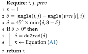
Algorithm A3 calculates the penalty for each direction change when Algorithm A1 searches a path. The penalty considered here is motivated by the radio wave propagation pathloss due to diffraction. Function on line 2 returns the edge direction from node i to node j. As illustrated in Figure 4a, there are only eight possible angles. Considering that a diffraction angle is between 0 and 180, lines 2 and 3 calculate the angular change () when going from node to node j via node i. If is larger than zero, lines 5–6 calculate the penalty. Function converts the angle in degree to radian. Penalty on line 6 is calculated via Equation (A1) which involves the Fresnel integral , calculated via Equation (A2) [40]. The Fresnel parameter in the Fresnel integral is calculated via Equation (A3). Assuming a wedge is present at node i that causes the diffraction, parameters and in Equation (A3) represent the distance between node and the wedge, and the distance between node j and the wedge, respectively. We simplify both and to be one. For more details about diffraction, interested readers are referred to Chapter 4.3 of the book by [40].
| Algorithm A3: Angular change penalty calculation. |
 |
References
- Björnson, E.; Hoydis, J.; Sanguinetti, L. Massive MIMO networks: Spectral, energy, and hardware efficiency. Found. Trends Signal Process. 2017, 11, 154–655. [Google Scholar] [CrossRef]
- Saleh, A.A.M.; Rustako, A.J.; Roman, R. Distributed antennas for indoor radio communications. IEEE Trans. Commun. 1987, 35, 1245–1251. [Google Scholar] [CrossRef]
- Larsson, E.G.; Edfors, O.; Tufvesson, F.; Marzetta, T.L. Massive MIMO for next generation wireless systems. IEEE Commun. Mag. 2014, 52, 186–195. [Google Scholar] [CrossRef] [Green Version]
- Björnson, E.; Sanguinetti, L. Making cell-free massive MIMO competitive with MMSE processing and centralized implementation. IEEE Trans. Wirel. Commun. 2020, 19, 77–90. [Google Scholar] [CrossRef] [Green Version]
- Zhu, Y.-H.; Monteyne, L.; Callebaut, G.; Rottenberg, F.; Van der Perre, L. Array Placement in Distributed Massive MIMO for Power Saving considering Radiation Pattern. In Proceedings of the 2021 IEEE 94th Vehicular Technology Conference (VTC2021-Fall), Norman, OK, USA, 27–30 September 2021; IEEE: Piscataway, NJ, USA, 2021; pp. 1–5. [Google Scholar]
- Ngo, H.Q.; Ashikhmin, A.; Yang, H.; Larsson, E.G.; Marzetta, T.L. Cell-free massive MIMO versus small cells. IEEE Trans. Wirel. Commun. 2017, 16, 1834–1850. [Google Scholar] [CrossRef] [Green Version]
- Shen, Y.; Tang, Y.; Kong, T.; Shao, S. Optimal antenna location for STBC-OFDM downlink with distributed transmit antennas in linear cells. IEEE Commun. Lett. 2007, 11, 387–389. [Google Scholar] [CrossRef]
- Gan, J.; Li, Y.; Zhou, S.; Wang, J. On sum rate of multi-user distributed antenna system with circular antenna layout. In Proceedings of the 2007 IEEE 66th Vehicular Technology Conference, Baltimore, MD, USA, 30 September–3 October 2007; IEEE: Piscataway, NJ, USA, 2007; pp. 596–600. [Google Scholar]
- Wang, X.; Zhu, P.; Chen, M. Antenna location design for generalized distributed antenna systems. IEEE Commun. Lett. 2009, 13, 315–317. [Google Scholar] [CrossRef]
- Ren, C.; Chen, M. On the optimal antenna placement for DAS systems. In Proceedings of the 2009 International Conference on Wireless Communications & Signal Processing, Nanjing, China, 13–15 November 2009; IEEE: Piscataway, NJ, USA, 2009; pp. 1–3. [Google Scholar]
- Qian, Y.; Chen, M.; Wang, X.; Zhu, P. Antenna location design for distributed antenna systems with selective transmission. In Proceedings of the 2009 International Conference on Wireless Communications & Signal Processing, Nanjing, China, 13–15 November 2009; IEEE: Piscataway, NJ, USA, 2009; pp. 1–5. [Google Scholar]
- Zhang, T.; Zhang, C.; Cuthbert, L.; Chen, Y. Energy efficient antenna deployment design scheme in distributed antenna systems. In Proceedings of the 2010 IEEE 72nd Vehicular Technology Conference-Fall, Ottawa, ON, Canada, 6–9 September 2010; IEEE: Piscataway, NJ, USA, 2010; pp. 1–5. [Google Scholar]
- Han, L.; Tang, Y.; Shao, S.; Wu, T. On the design of antenna location for OSTBC with distributed transmit antennas in a circular cell. In Proceedings of the 2010 IEEE International Conference on Communications, Cape Town, South Africa, 23–27 May 2010; IEEE: Piscataway, NJ, USA, 2010; pp. 1–5. [Google Scholar]
- Firouzabadi, S.; Goldsmith, A. Optimal placement of distributed antennas in cellular systems. In Proceedings of the 2011 IEEE 12th International Workshop on Signal Processing Advances in Wireless Communications, San Francisco, CA, USA, 26–29 June 2011; IEEE: Piscataway, NJ, USA, 2011; pp. 461–465. [Google Scholar]
- Park, E.; Lee, S.-R.; Lee, I. Antenna placement optimization for distributed antenna systems. IEEE Trans. Wirel. Commun. 2012, 11, 2468–2477. [Google Scholar] [CrossRef]
- Lee, C.; Park, E.; Lee, I. Antenna placement designs for distributed antenna systems with multiple-antenna ports. In Proceedings of the 2012 IEEE Vehicular Technology Conference (VTC Fall), Quebec City, QC, Canada, 3–6 September 2012; IEEE: Piscataway, NJ, USA, 2012; pp. 1–5. [Google Scholar]
- Zhang, W.; Diao, C.; Zhao, M.; Chen, M. Impact of path loss exponents on antenna location design for GDAS. In Proceedings of the 2012 IEEE 75th Vehicular Technology Conference (VTC Spring), Yokohama, Japan, 6–9 May 2012; IEEE: Piscataway, NJ, USA, 2012; pp. 1–5. [Google Scholar]
- Wang, H.; Wang, D.; Liu, R.; Xie, H.; Yang, Z. Antenna location design for distributed antenna systems with pilot contamination. In Proceedings of the 2013 International Conference on Wireless Communications and Signal Processing, Hangzhou, China, 24–26 October 2013; IEEE: Piscataway, NJ, USA, 2013; pp. 1–6. [Google Scholar]
- Yang, A.; Jing, Y.; Xing, C.; Fei, Z.; Kuang, J. Performance analysis and location optimization for massive MIMO systems with circularly distributed antennas. IEEE Trans. Wirel. Commun. 2015, 14, 5659–5671. [Google Scholar] [CrossRef] [Green Version]
- Kamga, G.N.; Xia, M.; Aïssa, S. Spectral-efficiency analysis of massive MIMO systems in centralized and distributed schemes. IEEE Trans. Commun. 2016, 64, 1930–1941. [Google Scholar] [CrossRef] [Green Version]
- Nayebi, E.; Rao, B.D. Access Point Location Design in Cell-Free Massive MIMO Systems. In Proceedings of the 2018 52nd Asilomar Conference on Signals, Systems, and Computers, Pacific Grove, CA, USA, 28–31 October 2018; IEEE: Piscataway, NJ, USA, 2018; pp. 985–989. [Google Scholar]
- Koyuncu, E. Performance gains of optimal antenna deployment in massive MIMO systems. IEEE Trans. Wirel. Commun. 2018, 17, 2633–2644. [Google Scholar] [CrossRef] [Green Version]
- Gopal, G.R.; Rao, B.D. Throughput and Delay Driven Access Point Placement. In Proceedings of the 2019 53rd Asilomar Conference on Signals, Systems, and Computers, Pacific Grove, CA, USA, 3–6 November 2019; IEEE: Piscataway, NJ, USA, 2019; pp. 1010–1014. [Google Scholar]
- Zhang, Y.; Dai, L. On the Optimal Placement of Base Station Antennas for Distributed Antenna Systems. IEEE Commun. Lett. 2020, 24, 2878–2882. [Google Scholar] [CrossRef]
- Gopal, G.R.; Villardi, G.P.; Rao, B.D. Is Vector Quantization Good Enough for Access Point Placement? In Proceedings of the 2021 55th Asilomar Conference on Signals, Systems, and Computers, Pacific Grove, CA, USA, 31 October–3 November 2021; IEEE: Piscataway, NJ, USA, 2021; pp. 1210–1214. [Google Scholar]
- Zhang, Y. Optimal Placement of Access Points for Infrastructure-based Wireless Communication Networks. Ph.D. Thesis, City University of Hong Kong, Hong Kong, China, 2021. [Google Scholar]
- Ammar, H.A.; Adve, R.; Shahbazpanahi, S.; Boudreau, G. Optimizing RRH Placement Under a Noise-Limited Point-to-Point Wireless Backhaul. In Proceedings of the ICC 2021-IEEE International Conference on Communications, Madrid, Spain, 7–11 December 2021; IEEE: Piscataway, NJ, USA, 2021; pp. 1–6. [Google Scholar]
- Gopal, G.R.; Nayebi, E.; Villardi, G.P.; Rao, B.D. Modified vector quantization for small-cell access point placement with inter-cell interference. IEEE Trans. Wirel. Commun. 2022, 1. [Google Scholar] [CrossRef]
- Atawia, R.; Ashour, M.; El Shabrawy, T.; Hammad, H. Indoor distributed antenna system planning with optimized antenna power using genetic algorithm. In Proceedings of the 2013 IEEE 78th Vehicular Technology Conference (VTC Fall), Las Vegas, NV, USA, 2–5 September 2013; IEEE: Piscataway, NJ, USA, 2013; pp. 1–6. [Google Scholar]
- Forooshani, A.E.; Lotfi-Neyestanak, A.A.; Michelson, D.G. Optimization of antenna placement in distributed MIMO systems for underground mines. IEEE Trans. Wirel. Commun. 2014, 13, 4685–4692. [Google Scholar] [CrossRef]
- Chen, C.-M.; Volski, V.; Van der Perre, L.; Vandenbosch, G.A.E.; Pollin, S. Finite Large Antenna Arrays for Massive MIMO: Characterization and System Impact. IEEE Trans. Antennas Propag. 2017, 65, 6712–6720. [Google Scholar] [CrossRef]
- Van der Perre, L.; Larsson, E.G.; Tufvesson, F.; Strycker, L.D.; Björnson, E.; Edfors, O. RadioWeaves for efficient connectivity: Analysis and impact of constraints in actual deployments. In Proceedings of the 2019 53rd Asilomar Conference on Signals, Systems, and Computers, Pacific Grove, CA, USA, 3–6 November 2019; pp. 15–22. [Google Scholar] [CrossRef] [Green Version]
- Lin, Y.; Yu, W.; Lostanlen, Y. Optimization of wireless access point placement in realistic urban heterogeneous networks. In Proceedings of the 2012 IEEE Global Communications Conference (GLOBECOM), Anaheim, CA, USA, 3–7 December 2012; IEEE: Piscataway, NJ, USA, 2012; pp. 4963–4968. [Google Scholar]
- Yun, Z.; Iskander, M.F. Ray tracing for radio propagation modeling: Principles and applications. IEEE Access 2015, 3, 1089–1100. [Google Scholar] [CrossRef]
- Minasian, A.; Adve, R.S.; Shahbazpanahi, S.; Boudreau, G. On RRH placement for multi-user distributed massive MIMO systems. IEEE Access 2018, 6, 70597–70614. [Google Scholar] [CrossRef]
- Minasian, A. Optimal Design of Multi-user Distributed Massive MIMO Systems. Ph.D. Thesis, University of Toronto, Toronto, ON, Canada, 2019. [Google Scholar]
- Nemhauser, G.L.; Wolsey, L.A. Integer Programming and Combinatorial Optimization; Springer: Berlin, Germany, 1988; Volume 191. [Google Scholar]
- Glover, F.W.; Kochenberger, G.A. Handbook of Metaheuristics; Springer Science & Business Media: Berlin, Germany, 2006; Volume 57. [Google Scholar]
- Lodro, M.M.; Majeed, N.; Khuwaja, A.A.; Sodhro, A.H.; Greedy, S. Statistical channel modelling of 5G mmWave MIMO wireless communication. In Proceedings of the 2018 International Conference on Computing, Mathematics and Engineering Technologies (iCoMET), Sukkur, Pakistan, 3–4 March 2018; IEEE: Piscataway, NJ, USA, 2018; pp. 1–5. [Google Scholar]
- Molisch, A.F. Wireless Communications; John Wiley & Sons: Hoboken, NJ, USA, 2012; Volume 34. [Google Scholar]
- Dijkstra, E.W. A note on two problems in connexion with graphs. Numer. Math. 1959, 1, 269–271. [Google Scholar] [CrossRef] [Green Version]
- Hart, P.E.; Nilsson, N.J.; Raphael, B. A formal basis for the heuristic determination of minimum cost paths. IEEE Trans. Syst. Sci. Cybern. 1968, 4, 100–107. [Google Scholar] [CrossRef]
- Floyd, R.W. Algorithm 97: Shortest path. Commun. ACM 1962, 5, 345. [Google Scholar] [CrossRef]
- Liu, L.; Oestges, C.; Poutanen, J.; Haneda, K.; Vainikainen, P.; Quitin, F.; Tufvesson, F.; De Doncker, P. The COST 2100 MIMO channel model. IEEE Wirel. Commun. 2012, 19, 92–99. [Google Scholar] [CrossRef] [Green Version]
Figure 1.
The access point (AP) placement optimization problem includes two parts: problem modeling (the blocks within the dashed line) and solver development. This paper focuses on the problem modeling part. We discuss different setups for the distributed massive multiple-input multiple-output (D-mMIMO) system and different ways for modeling the environment. Four approaches for calculating the channel gain at each user location have been considered: a ray-tracing simulator (RTS)-based model and a Euclidean distance-based model, both of which are from the literature, and two graph-based models which are proposed in this paper.

Figure 2.
Example of an area to be covered by a D-mMIMO deployment. The dashed line indicates the border of the coverage region. The black dots are the potential user locations that need to be covered by the signal, hence a discretization of the continuous area into a grid. The D-mMIMO system has multiple APs. The black dots next to buildings also indicate the potential locations for deploying the APs.

Figure 3.
Elevation plane gain patterns (dBi) of the considered isotropic element and patch element. (a) Isotropic antenna; (b) Patch antenna.
Figure 3.
Elevation plane gain patterns (dBi) of the considered isotropic element and patch element. (a) Isotropic antenna; (b) Patch antenna.

Figure 4.
(a) shows the eight possible broadside directions for the array when mounting an AP on a wall. (b) is an example of the broadside directions for different potential AP locations. The dark gray area represents a building. The black dots next to the building are the potential AP locations. The blue arrows indicate the broadside directions for each potential AP location.

Figure 5.
The limitations of the Euclidean distance-based model. The blue arrow represents the broadside direction for the array at the AP location. The green straight line indicates the Euclidean distance between user location i and AP location l. The orange polyline indicates a possible propagation path from AP location l to user location i.
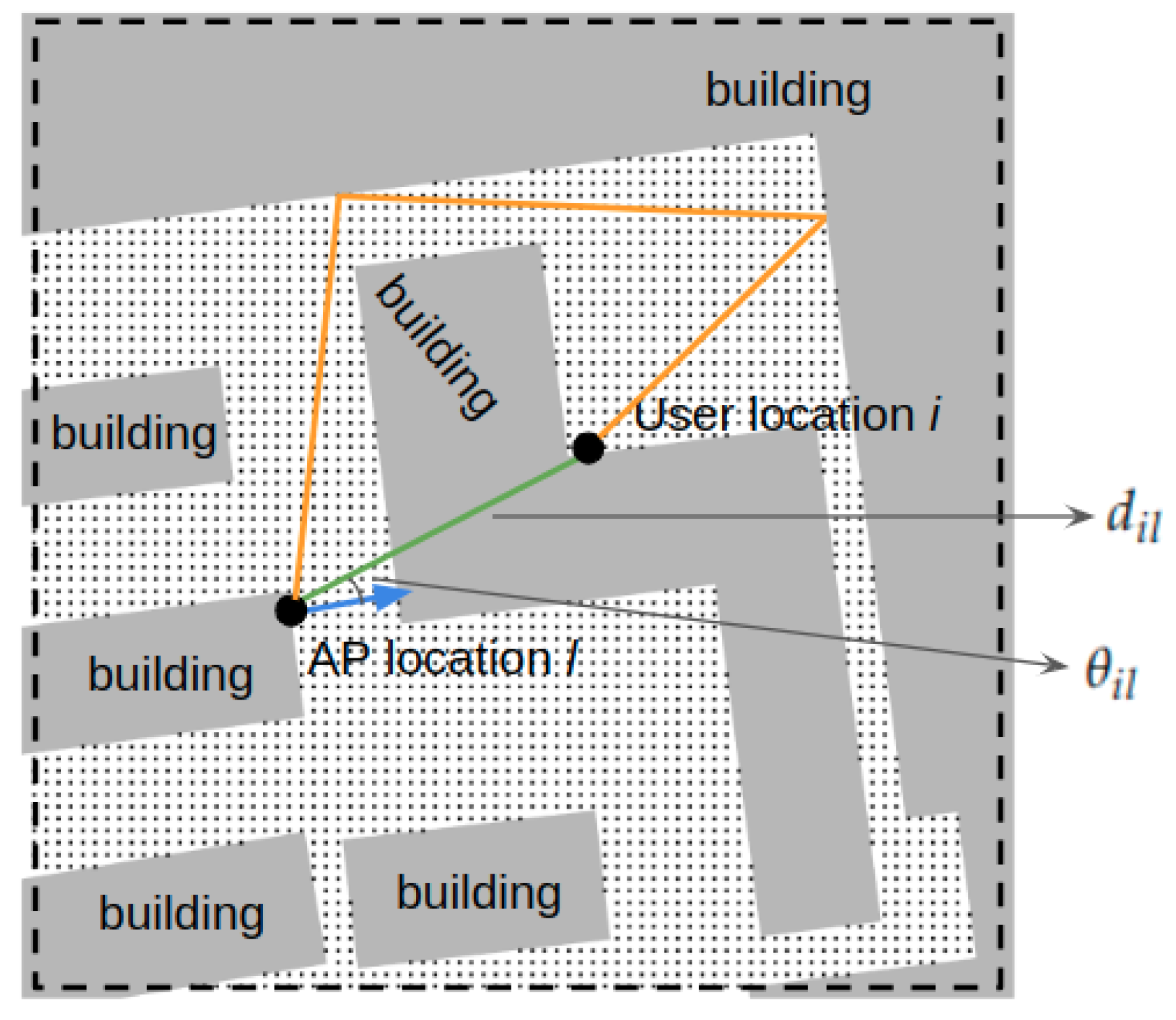
Figure 6.
An example of the graph for capturing environment information on the map. The nodes in the graph are one meter apart and directly connected to their neighbor nodes via edges. The figure on the right zooms in on the graph. The highlighted lines illustrate the eight edges that connect a node with all of its neighbor nodes. The dashed line in the left figure indicates the coverage region. Each node within the coverage region is associated with a generated location mentioned in Section 2.

Figure 7.
The procedure for executing the experiments with different channel models.

Figure 8.
Comparison between the full coverage region and simplified coverage region regarding the total required transmit power. When considering a full coverage region or a simplified one, the total transmit power simulated via the RTS is very similar. This confirms that the simplified coverage region contains the user locations which receive the overall lowest channel gain. (a) Map 1; (b) Map 5.

Figure 9.
Comparison between the full coverage region and simplified coverage region regarding the heatmaps of the average received signal power at user locations. The red spots are the APs. The orange spots are the user locations that receive the overall lowest signal power. (a) Full; (b) Simplified.

Figure 10.
The simplified coverage regions of the five maps used in the experiments. (a) Coverage region: ; (b) Coverage region: ; (c) Coverage region: ; (d) Coverage region: ; (e) Coverage region: .
Figure 10.
The simplified coverage regions of the five maps used in the experiments. (a) Coverage region: ; (b) Coverage region: ; (c) Coverage region: ; (d) Coverage region: ; (e) Coverage region: .
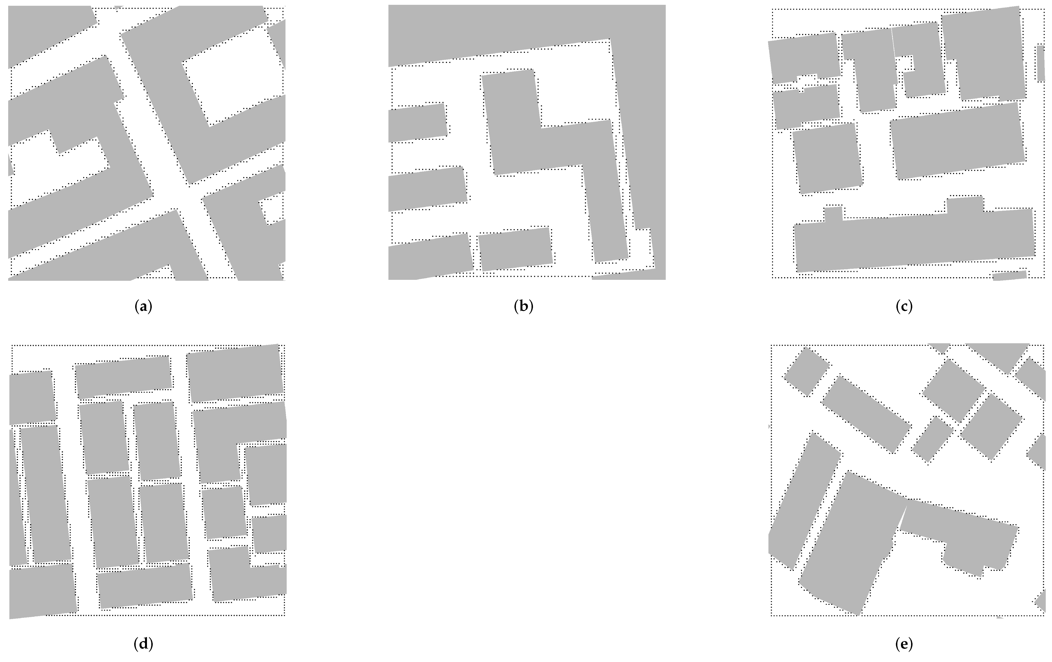
Figure 11.
Impact of the total AP number on the D-mMIMO system’s performance (128 antennas in total) with optimized AP placements on the average relative power saving when the D-mMIMO system is equipped with four APs compared with one or two APs over all the maps.
Figure 11.
Impact of the total AP number on the D-mMIMO system’s performance (128 antennas in total) with optimized AP placements on the average relative power saving when the D-mMIMO system is equipped with four APs compared with one or two APs over all the maps.

Figure 12.
Significance of considering radiation pattern for AP placement optimization. The average relative power saving when generating AP placements considering the radiation pattern compared with the situation where we do not consider the radiation pattern, using patch antennas.
Figure 12.
Significance of considering radiation pattern for AP placement optimization. The average relative power saving when generating AP placements considering the radiation pattern compared with the situation where we do not consider the radiation pattern, using patch antennas.

Figure 13.
Heatmaps of the RTS-simulated received signal power at user locations when using the optimal AP placements generated using different channel models for map 5, using patch antennas. The red spots are the APs. The orange spots are the user locations that receive the overall lowest signal power. (a) Euclidean distance-based model; (b) Shortest path-based model; (c) Angular penalty-based model; (d) RTS-based model.
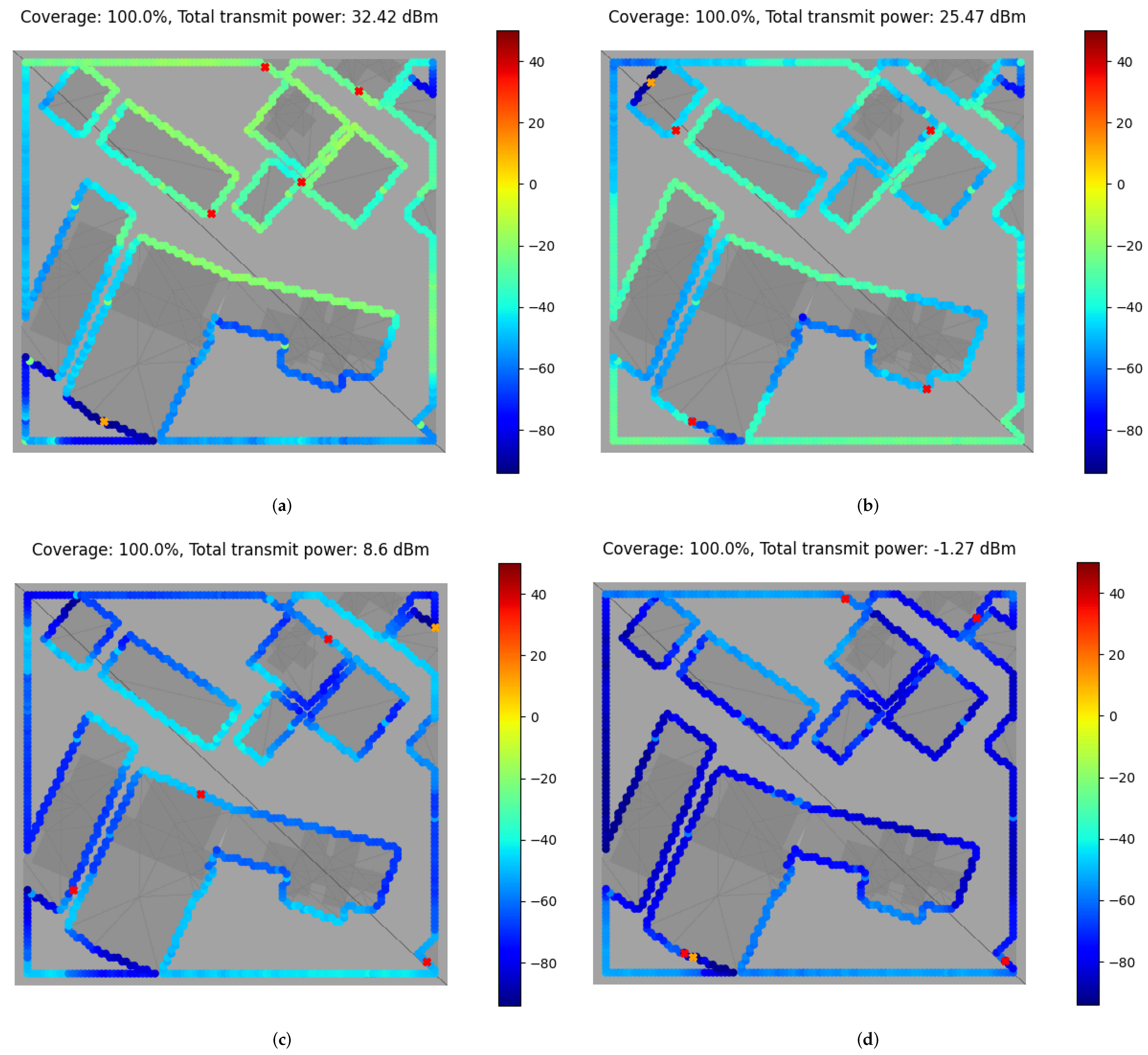
Figure 14.
Comparison of different channel models. The average relative power saving when using the AP placements generating via the shortest path-based model, angular penalty-based model or the RTS-based model compared with the Euclidean distance-based model. (a) Isotropic; (b) Patch.
Figure 14.
Comparison of different channel models. The average relative power saving when using the AP placements generating via the shortest path-based model, angular penalty-based model or the RTS-based model compared with the Euclidean distance-based model. (a) Isotropic; (b) Patch.

Table 1.
Notation.
| Parameters | |
|---|---|
| set of potential AP locations in the region | |
| set of potential user locations in the region | |
| T | total number of AP in the D-mMIMO deployment |
| minimum average received signal power, required at each user location | |
| V | signal coverage level as a percentage |
| Variables | |
| non-negative, transmitted power per ap | |
| binary, equals one if an AP is deployed at location l | |
| binary, equals one if user location i is covered with sufficient signal | |
Table 2.
Parameter settings.
| General: | Minimum required transmit power () | dBm |
| Center frequency | GHz | |
| Total number of antennas in the system | 128 | |
| Signal coverage levels (V) | 100%, …, 91% and 90% | |
| RTS: | Height of each ap | 30 |
| Height of each user location | ||
| Bandwidth | 100 MHz | |
| Total number of sub-carrier frequencies | 10 |
Table 3.
Computation time (s) of RTS for evaluating all the channels for an AP placement considering the full or simplified coverage regions. Different AP placements, antenna types, and maps are tested in the experiments. The first column is for the indexes of AP placements.
Table 3.
Computation time (s) of RTS for evaluating all the channels for an AP placement considering the full or simplified coverage regions. Different AP placements, antenna types, and maps are tested in the experiments. The first column is for the indexes of AP placements.
| AP Placements | Map 1 | Map 5 | ||||||
|---|---|---|---|---|---|---|---|---|
| Isotropic | Patch | Isotropic | Patch | |||||
| Full | Simplified | Full | Simplified | Full | Simplified | Full | Simplified | |
| 0 | 4354 | 974 | 4237 | 998 | 9615 | 1682 | 9876 | 1741 |
| 1 | 4279 | 1098 | 4274 | 1017 | 9415 | 1639 | 9616 | 1638 |
| 2 | 4255 | 1061 | 4209 | 975 | 8939 | 1536 | 9054 | 1593 |
| 3 | 4481 | 1014 | 4411 | 1067 | 9253 | 1693 | 9353 | 1821 |
| 4 | 4340 | 1007 | 4296 | 981 | 10,189 | 1697 | 10,407 | 1943 |
| 5 | 4386 | 1031 | 4465 | 1013 | 10,174 | 1652 | 10,379 | 1676 |
| 6 | 4423 | 1063 | 4432 | 1008 | 9795 | 1716 | 10,027 | 1741 |
| 7 | 4359 | 1007 | 4307 | 977 | 9756 | 1679 | 9863 | 1733 |
| 8 | 4158 | 1064 | 4240 | 985 | 10,118 | 1861 | 10,513 | 1832 |
| 9 | 4349 | 1021 | 4316 | 1020 | 10,029 | 1689 | 10,578 | 1680 |
Table 4.
The average time required by different models to evaluate the channels for all the possible AP placement in a simplified coverage region.
Table 4.
The average time required by different models to evaluate the channels for all the possible AP placement in a simplified coverage region.
| Channel Models | Time (min) |
|---|---|
| Ray-tracing simulator (RTS)-based model | Around 600 |
| Euclidean distance-based model | 1.2 |
| Shortest path-based model | 1.2 |
| Angular penalty-based model | 1.2 |
Publisher’s Note: MDPI stays neutral with regard to jurisdictional claims in published maps and institutional affiliations. |
© 2022 by the authors. Licensee MDPI, Basel, Switzerland. This article is an open access article distributed under the terms and conditions of the Creative Commons Attribution (CC BY) license (https://creativecommons.org/licenses/by/4.0/).
Share and Cite
MDPI and ACS Style
Zhu, Y.-H.; Callebaut, G.; Çalık, H.; Van der Perre, L.; Rottenberg, F. Energy Efficient Access Point Placement for Distributed Massive MIMO. Network 2022, 2, 288-310. https://doi.org/10.3390/network2020019
AMA Style
Zhu Y-H, Callebaut G, Çalık H, Van der Perre L, Rottenberg F. Energy Efficient Access Point Placement for Distributed Massive MIMO. Network. 2022; 2(2):288-310. https://doi.org/10.3390/network2020019
Chicago/Turabian StyleZhu, Yi-Hang, Gilles Callebaut, Hatice Çalık, Liesbet Van der Perre, and François Rottenberg. 2022. "Energy Efficient Access Point Placement for Distributed Massive MIMO" Network 2, no. 2: 288-310. https://doi.org/10.3390/network2020019