
Development of a Toolchain for Automated Optical 3D Metrology Tasks


1
Faculty of Electrical Engineering, University of Applied Sciences Augsburg, An der Hochschule 1, 86161 Augsburg, Germany
2
Fraunhofer Research Institute for Casting, Composite and Processing Technology IGCV, Am Technologiezentrum 2, 86159 Augsburg, Germany
*
Author to whom correspondence should be addressed.
†
These authors contributed equally to this work.
Metrology 2022, 2(2), 274-292; https://doi.org/10.3390/metrology2020017
Submission received: 8 April 2022
/
Revised: 9 May 2022
/
Accepted: 16 May 2022
/
Published: 31 May 2022
(This article belongs to the Special Issue Advances in Portable 3D Measurement)
Abstract
:Modern manufacturing processes are characterized by growing product diversities and complexities alike. As a result, the demand for fast and flexible process automation is ever increasing. However, higher individuality and smaller batch sizes hamper the use of standard robotic automation systems, which are well suited for repetitive tasks but struggle in unknown environments. Modern manipulators, such as collaborative industrial robots, provide extended capabilities for flexible automation. In this paper, an adaptive ROS-based end-to-end toolchain for vision-guided robotic process automation is presented. The processing steps comprise several consecutive tasks: CAD-based object registration, pose generation for sensor-guided applications, trajectory generation for the robotic manipulator, the execution of sensor-guided robotic processes, test and the evaluation of the results. The main benefits of the ROS framework are readily applicable tools for digital twin functionalities and established interfaces for various manipulator systems. To prove the validity of this approach, an application example for surface reconstruction was implemented with a 3D vision system. In this example, feature extraction is the basis for viewpoint generation, which, in turn, defines robotic trajectories to perform the inspection task. Two different feature point extraction algorithms using neural networks and Voronoi covariance measures, respectively, are implemented and evaluated to demonstrate the versatility of the proposed toolchain. The results showed that complex geometries can be automatically reconstructed, and they outperformed a standard method used as a reference. Hence, extensions to other vision-controlled applications seem to be feasible.
1. Introduction
Robotic process automation is a growing field with applications in different industrial sectors. Typical tasks range from automated optical inspection for quality control in industrial production to vision-controlled process automation in assembly. One of the main challenges is flexibility with respect to varying product properties, changing process environments or human–machine interaction, while manufacturing and assembly are areas where fully automated robotic systems are already well-established, quality control is a field that remains dominated by semi-automatic inspection processes, which combine manual tasks with robotic assistance.
High product variance, small lot sizes as well as the complexity of manipulation tasks, such as peg-in-hole processes have thus far prevented the use of robotic process automation especially in small- and medium-sized companies. The demand for frequent adaptations of control algorithms and programs can only be addressed by highly skilled workers. Unfortunately, human intervention remains error prone, time consuming and expensive. Hence, it would be desirable to equip vision-based control and inspection systems with more autonomous planning and task execution capabilities.
Different frameworks, such as the Robot Operating System (ROS) [1], an independent operating system for closed loop robotic systems, and software libraries for sensor data processing, such as OpenCV [2] and PointCloudLibrary [3], have been developed to provide open access to algorithms. Nevertheless, integrated approaches to combine object and sensor data processing with task and trajectory planning as well as the evaluation of measurement results are still scarcely available. In addition, the fusion of different data sources, e.g., different sensor systems or CAD and sensor data, is still an open topic in many applications.
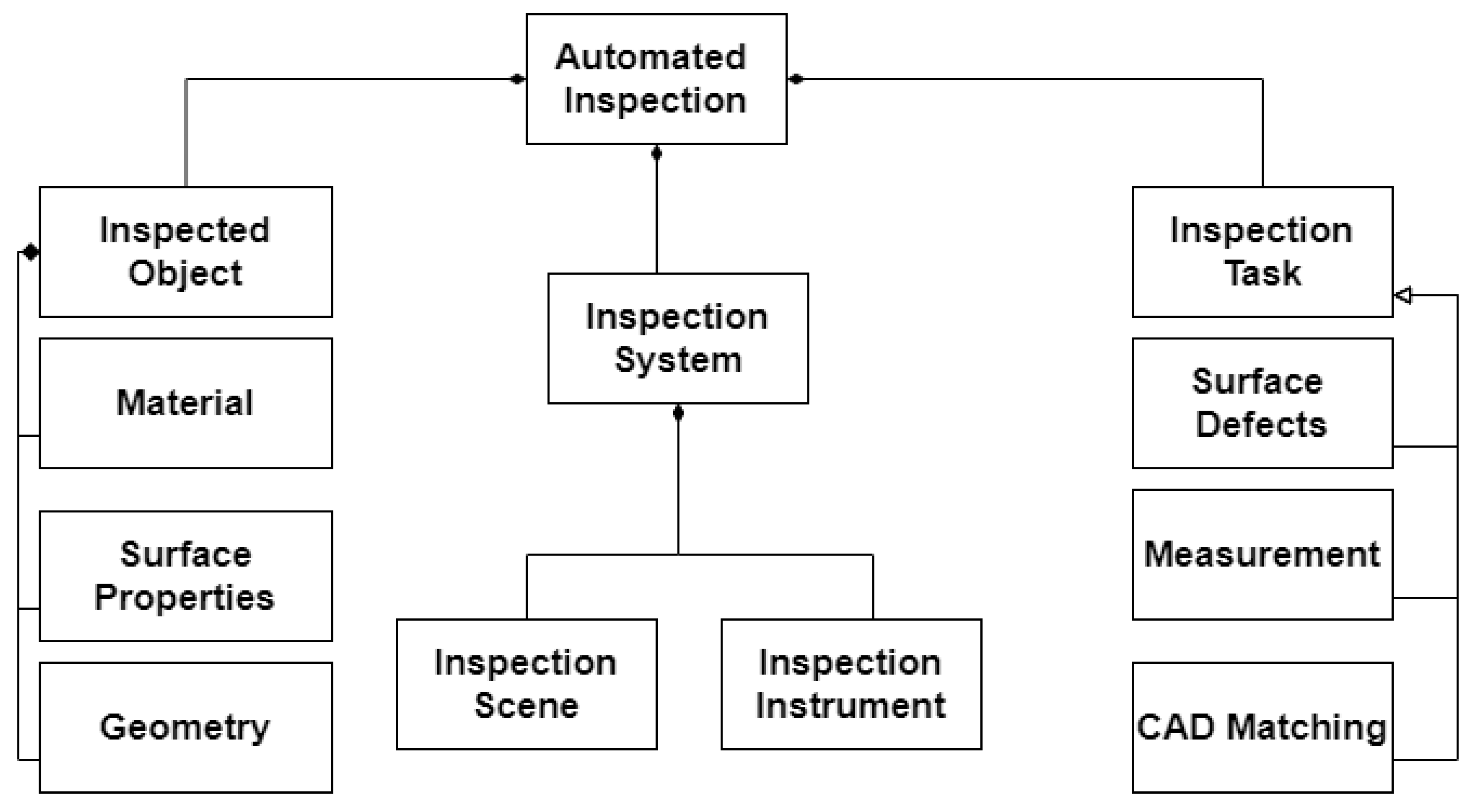
In the particular case of quality inspection, typical challenges for process automation are nonstandardized inspection procedures due to high variations in object geometry, surface properties and customer requirements. As shown in Figure 1, quality inspection is a process involving the following entities:
- Inspected object.
- Inspection system.
- Inspection task.
The inspected object is characterized by its physical properties. The most important is its geometry as this directly affects all measurement systems. During the entire inspection task, defined spatial configurations between the selected measurement system and the surface of the inspected object have to be maintained. The material and surface properties of the inspected object also have to be considered for the planning of an inspection task because they affect the suitability of an inspection system to capture the surface and determine the accuracy of the measurement.
The inspection system generates the data to be evaluated by the inspection task. Depending on the task an appropriate inspection instrument has to be selected. The instrument comprises of the measurement system itself as well as the according manipulator. The main task of the manipulator is to position the measurement system in a defined configuration relative to the inspected object and keep this configuration stable. The inspection scene entails all environmental aspects of the inspection, such as the lighting, temperature and humidity.
These parameters have to be kept in a range where the instrument generates data that can be used in subsequent evaluation tasks. The inspection task specifies how the inspection system has to be arranged around the inspected object in order to generate measurement results and and ensure these data are further evaluated in order to produce a representative result.
Depending on the inspection tasks different sources of information about the inspected object need to be combined for correct evaluation. Possible tasks range from 3D measurements on the object to be inspected over matching of CAD-models to the detection of defects in the inspected object. As an example, the task of finding surface defects of a defined type is briefly explained. Depending on the size and shape of the surface defects, an appropriate camera can be selected. The surface properties of the object (e.g., reflective/non-reflective) set the inspection scene with regards to the illumination and the position of the camera relative to the surface. Most other inspection processes can be described by specific instances of the named components in a similar way.
Based on the idea of breaking up complex processes into small, clearly defined tasks, the main contribution of this paper can be described as follows: A flexible end-to-end toolchain for visual inspection processes was developed that can be used to acquire and analyze measurement data in a fully automated fashion with interfaces to different robotic manipulator systems and simulation capabilities for the robotic inspection task. The main focus was to create a universal toolchain that can be adopted for different inspection systems, inspected objects and inspection tasks. To demonstrate the versatility of the developed toolchain, an exemplary application in the area of surface reconstruction was chosen; however, the concept can seamlessly be applied to other inspection tasks as well.
This paper is organized as follows: First, we summarize the state of the art of vision-based quality inspection and task planning for robotic process automation in industrial applications. Section 3 presents the universal robotic system architecture for automated vision-based process control and inspection and the integrated processing toolchain. For the specific use case of the surface reconstruction of a cast component from the automotive sector, the integrated algorithms for feature extraction and viewpoint generation are also outlined.
The results of the successive processing phases and the final reconstruction accuracy are presented in Section 4. The validity of the proposed end-to-end toolchain for robotic process automation in industrial applications is discussed, and extensions to further apply and test the toolchain are outlined in Section 5.
2. State of the Art
Various inspection systems for 3D metrology have been proposed in the literature. The capabilities of a flexible 3D laser scanning system using a robotic arm were demonstrated in [4]. Similarly, a 3D reconstruction automation system was introduced in [5], and an in-line 3D inspection system was presented in [6]. Wang et al. developed an inspection system for large-scale complex geometric parts in [7]. Almadhoun et al. conducted an extensive survey of robot-based inspection systems [8]. Their main finding was that programming environments for applications set very rigid boundaries and do not allow for flexible adaptations of the tasks of such systems. There are some approaches towards plug-and-play solutions for robotic applications [9]; however, no universal framework has been established yet. The limitation of most systems is that their rigid architecture is tailored for a particular task and hence cannot easily be extended or adapted to meet the requirements of different use cases.
Model-based viewpoint generation techniques are a class of techniques that use the geometric information about the object that is to be inspected and output a set of suitable viewpoints for the complete inspection task [10]. Based on how this geometric information is made available, these techniques can be subdivided into two categories. The first category uses a CAD model of the object to be inspected as input.
The standard triangle language (STL) file format is widely used in industry as a quasi-standard for the exchange of geometric data in form of surface meshes. This file format does not contain any explicit information about curvatures or neighborhood information about the meshes [11].
Wu et al. proposed a laser-scanner-based optical inspection system, which takes the geometrical information in form of a STL file as input [12] and subsequently improved their algorithms to handle more complex geometries [13]. If a different CAD file format that contains both curvature and surface normal information is available, other techniques, such as those demonstrated by Liu et al. [14], can be used.
When the CAD model of the object is not available, Coordinate Measuring Machines (CMMs) or 3D-scanners can be used to create a digital model of the object. Such models are often created in the form of point clouds. A point cloud can also be extracted by subsampling a surface mesh. The geometric information of the point cloud then corresponds to the geometric information of the object.
Point clouds have been gaining popularity among researchers in the field of inspection planning because operations based on point clouds are computationally less expensive than those on meshes. This was exploited by Zou et al. to create isoparametric tool paths on surfaces [15]. The structure of point clouds can be used to create and optimize viewpoints for image acquisition systems satisfying different needs, e.g., surface coverage ratio [16]. Ref. [17] developed an adaptive algorithm for autonomous 3D surface reconstruction based on point clouds. The trajectories of the robotic inspection system were generated and simulated in MATLAB.
Feature points can be identified in point clouds to mark points with special properties. These properties can, e.g., concern surface variations in the vicinity or point densities in the surrounding volume element. They can be estimated by using numerical optimization approaches or other methods, such as Voronoi-based algorithms. A Voronoi-based method for the extraction of normals from a point cloud was proposed by Amneta and Bern in [18]. This was then extended to ensure robustness against noise in [19]. Mérigo et al. built upon this work and proposed a method that can not only provide the normal information of the point cloud but also the underlying curvature information [20].
The use of neural networks for feature point extraction from point clouds has recently gained popularity. PointNet [21], PointNet++ [22] and Dynamic Graph Convolutional Neural Networks (DGCNN) [23] are primary neural network architectures for convolutional operations on point cloud data. The DGCNN architecture was used for feature extraction in [24,25]. A PointNet-based architecture for feature extraction was implemented in [26].
3. Methods
The foundation for a modular and flexible toolchain for component inspection is a continuous and fully digital representation of the inspection entities. This section explains the digital model and breaks down the different tasks along the toolchain. The digital system covers the inputs to the system, the necessary processing steps and the execution of the system using ROS tools. The application-specific evaluation of the acquired measurement results is explained in Section 4.
3.1. Toolchain
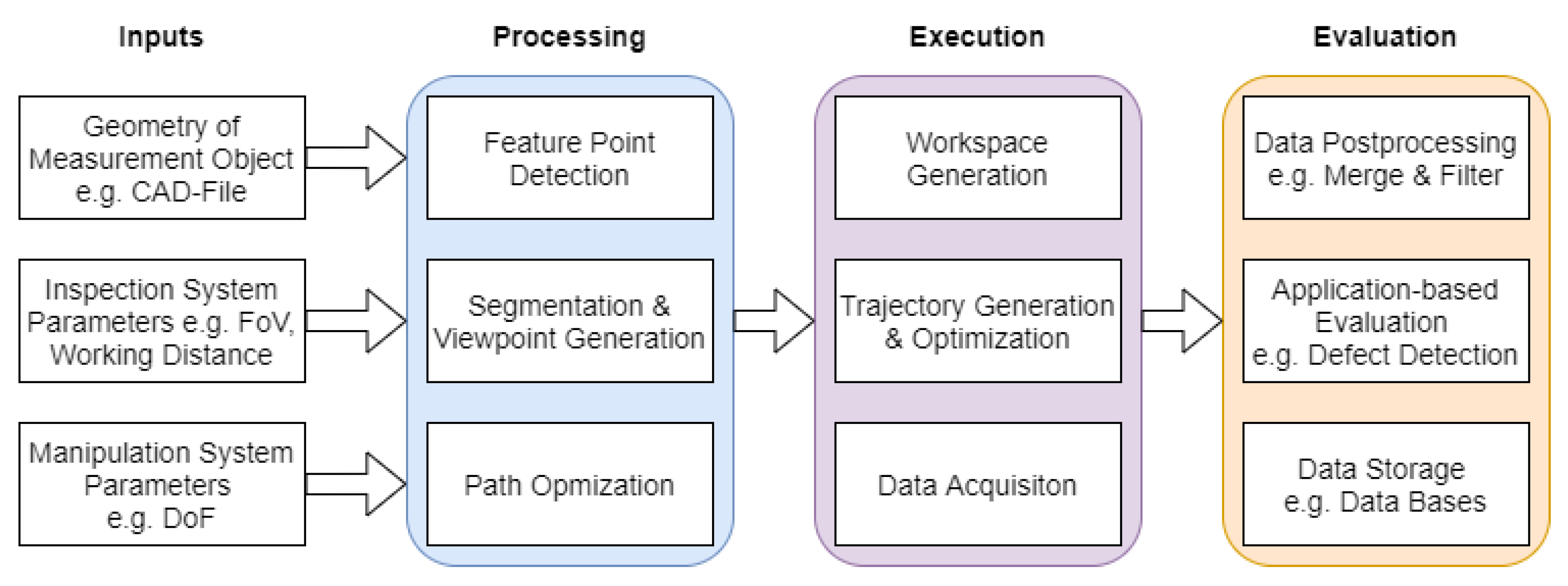
The term toolchain refers to the sequence of all operations involved in an automated inspection process. Figure 2 depicts the developed toolchain for an automated optical metrology task. The toolchain can be subdivided into three procedural units—processing, execution and evaluation. The processing step takes the geometry of the measurement object, parameters of the inspection system and the manipulator system parameters as inputs and performs feature detection, segmentation and viewpoint generation, as well as path optimization. Data acquisition is conducted in the execution step. The execution depends on the ROS-based architecture described in Section 3.4. This is followed by an application-specific evaluation step. In the following, the methods employed in each of the steps for this specific application are described.
3.2. Inputs
3.2.1. Geometry
For any kind of inspection planning the key information is that about the object to be analyzed. Information about the geometry can be provided in multiple formats, each with their own depth of information. As explained in Section 2, there are two main forms of geometry representations—meshes and point clouds.
Mesh files contain information about the planar elements on the surface of the object. These polygons consist of points (vertices), which are connected by lines creating shapes with at least three corners [27]. In the case of a polygon with exactly three corners, the mesh M can also be referred to as a simplex mesh. A widely used file format for simplex meshes is the STL format. This file format exists in human readable ASCII or binary form. As of its performance advantages the binary form is more commonly used. The structure of an STL file is independent of the representation form and consists of an unordered list of polygons. Each polygon has the following two attributes: the normal vector and the according vertices .
Point clouds, on the other hand, do not contain information about the connections between points but only about the vertices. A point cloud is an unordered set of three-dimensional points in a frame of reference (Cartesian coordinate system) on the surface of objects.
Depending on the field or software used, there are many different file formats for storing the spatial information in form of point clouds. Some of the most used include OBJ, STEP and PCD file formats. Some file formats support the storing of additional information about points, such as color, normal direction or analysis results in form of scalar fields.
3.2.2. Inspection System
In order to perform any kind of inspection task a measurement system is needed. Although different measurement systems produce different outputs their main features can be described in a generalized form. Independent of the data produced, every measurement system has an optimal working distance for a specific type of operation that can be determined either analytically or through experiments. Depending on the kind of signal-guiding system mounted on the individual measurement system, the field of view (FOV) parameters can be determined. Examples of these parameters are the horizontal and vertical opening angles of camera optics or the directional angle of the wedge of ultrasonic transducers as well as the working distance.
The determination of the working parameters for the systems to be used are not part of this contribution but were found through experiments prior to the measurements. In order to be able to create consistent and complete representations of the measurement results, the signal output of an inspection system can be treated as a matrix representation with its reference point in the principal point of the measurement system. Using this kind of representation, a single-source ultrasonic transducer can be treated in the same way as a 3D scanning system.
3.2.3. Manipulation System
For complex inspection tasks, modern manipulation system with several degrees of freedom have to be used to be able to reach the acquisition poses around the inspected object. Six degrees of freedom (DOF) robotic arms are the most frequently used manipulator type in the inspection of medium-sized components. Such robotic systems can also be referred to as serial-link manipulators, which consist of rigid links connected by joints. Every joint moves the link it is connected to along its degree of freedom and can either be categorized as a rotational (revolute) or translational (prismatic) joint. The entire kinematic chain of such a manipulation system connects the robot base with its tool tip, more formally known as its end effector.
Taking the example of the articulated manipulator, a uniquely defined pose in Cartesian space can be reached by setting the joint angles within their ranges . The entire space of possible valid combinations of joint angles is called joint space ,
The sequential addition of poses given by the individual joint angles is referred to as Forward Kinematics and always yields a unique solution for a pose in Cartesian space. The reverse operation of finding a set of valid joint angles for a given pose in task space is called Inverse Kinematics,
Figure 3 shows the relations between Joint Space and Task Space through Forward and Inverse Kinematics respectively.
For the six-DOF serial robotic arm, there can be poses of the end-effector in task space for which no unique solution for a combination of joint angles exist; however, multiple or even infinitely many combinations can be found. Finding valid combinations analytically can be cumbersome. Frameworks, such as ROS, use numerical solvers to find solutions for these systems of equations.
3.3. Processing
The previously explained input parameters are handled in the following processing step. This process consists of three single operations:
- Feature Point Detection.
- Segmentation and Viewpoint Generation.
- Path Optimization.
3.3.1. Feature Point Detection
The developed system is characterized by its high flexibility that allows for application-specific customization of different functional blocks. To demonstrate this flexibility, two different methods that can be employed for feature point detection, Voronoi Covariance Measure (VCM) and Dynamic Graph Convolutional Neural Network (DGCNN), and their integration in the proposed toolchain are presented.
Feature Point Detection Using Voronoi Covariance Measure
The estimation of the curvature of the underlying surface denoted by the point cloud relates to the estimation of the shape of the Voronoi cell around an individual point [20]. Let be the points of a point cloud, then the Voronoi cell of a point is defined is a region in 3D space containing all the points , where the following property holds true:
If a point lies on a sharp edge, the shape of the Voronoi cell is that of a triangle. At the corner, the Voronoi cell is cone-shaped, and it is pencil-shaped if the point lies on the surface. This shape information can be captured using the eigenvalues of the Voronoi cell because the ratio of the eigenvalues determines the shape of the underlying surface. For example, if a point lies on a sharp edge, it will have two larger eigenvalues and one smaller one. The covariance matrix can be used for this analysis. Recall that, for a bounded finite volume , the covariance matrix can be calculated with respect to a point as
The eigenvectors of the covariance matrix capture the principal axes of the region, and their ratio captures its anisotropy. By nature, Voronoi cells are globally influenced. Voronoi cells of the outer points of the point cloud are unbounded because they extend infinitely in . To extract the local information from these cells, the notion of intersecting ball is introduced by Merigot et al. [20]. Formally, the ball around a point with radius r is defined as
To bound the Voronoi cell , consider its intersection with the ball , . Then, the Voronoi Covariance Measure is defined as:
The of any point in the point cloud C is a symmetric matrix that contains information about the Voronoi cell of the point. To address the noise-related deviation of the shape of the Voronoi cell, the VCM of the points in the spherical neighborhood with radius R of point are summed together. Formally,
for some that can be used as a design parameter. Once the VCM has been calculated, the features can be extracted using the algorithm derived in [20]. The choice of suitable ball radii r, neighborhood radii R and threshold parameters is essential for valid results. The selection of r depends on the expected geometry of the underlying point cloud. Provided that r is a smaller than the one-sided reach of the object, all the sharp edges will be identified, and its value should be chosen as the largest possible lower bound on the one-sided reach of the underlying surface.
The neighborhood radius R should be chosen in such a way that every ball with contains at least 20 to 30 points. The point is a feature point if the ratio of the eigenvalues fulfills the following condition:
where is the maximum detectable dihedral angle. In order to select the point on the curved surface with dihedral angle of , the following criteria should be fulfilled [20]:
The mathematical proof as well as further explanations for the statements in this section can be found in [20].
Feature Point Detection Using Dynamic Graph Convolutional Neural Network
The concept of Dynamic Graph Convolutional Neural Networks was introduced by Wang et al. [23], and its architecture is shown in Figure 4. The EdgeConv operation builds the core of the feature point detection model used in this paper. The model takes a three-dimensional point cloud as input. The point cloud is passed through three layers of EdgeConv. The output of each layer is then pooled together and then passed through a Multi-Layer Perceptron (MLP). The output of the MLP is then passed through a linear layer, called Output, which calculates a probability value for the points of the point cloud. This result is subsequently used to determine whether a point is a feature-point or a non-feature point.
The model is implemented using the PyTorch Geometric Library. The EdgeConv operator is implemented using a Multi-Layer Perceptron consisting of linear layers, which are arranged sequentially. ReLU is used as the activation function, and batch normalization is enabled. The hyperparameter k, which determines the number of nearest neighbors considered by EdgeConv operator is set to 30. Random noise is introduced in the point cloud by translating and rotating the points of the point cloud up to mm/m and ° along the , or axis, respectively.
This ensures that the model can deal with perturbations in the acquired data. The point cloud is normalized into a unit sphere, for better generalization. The model is then trained for feature detection using the ABC dataset. The ABC dataset is a collection of one million Computer Aided Design (CAD) models for research of geometric deep-learning methods and applications [29].
Each model in the dataset has details on explicitly parameterized curves and surfaces and provides ground truth for patch segmentation, shape reconstruction and geometric feature detection. Sharp feature curves are defined in the ABC dataset as the interface between any two regions for which normal orientation for either region differs by more than 18°. This places the inherent limitation on the model that it can only detect sharp features that are greater than 18°.
3.3.2. Segmentation
Segmentation is the process of subdividing the geometry under inspection into several regions with similar properties, further on referred to as segments S. Any segmentation algorithm that satisfies the application specific requirements can be selected for this process.
Based on the satisfying results of the Topological Mode Analysis Tool (ToMATo) algorithm and visual feedback possibilities, it was chosen for this demonstrative application. ToMATo is a segmentation algorithm based on persistence homology, which comes with theoretical guarantees and visual feedback [30]. Regarding these properties, the ToMATo algorithm is a good choice for the segmentation of point clouds.
For the initial segments, the geodesic distance of Rips complexes between each point in the point cloud and its nearest feature point is used. The initial segments are then refined using the cosine similarity measure to subdivide each segment according to their normal deviation. The cosine similarity is calculated as the Euclidean dot product between each point in the segment and the mean normal of the segment.
3.3.3. Viewpoint Generation
Once the segments of the point cloud C have been determined using an appropriate algorithm, viewpoints for the individual segments can be generated. A viewpoint is defined as a 4 × 4 homogeneous matrix that describes the position and orientation of the reference point of a measurement system with respect to the global coordinate system of the inspection scene. It is assumed that the measurement system has a principal direction that can be used to position the device in space with respect to the inspected object. This principal direction is aligned with the mean normal of each individual segment.
For each point , the normal with respect to the object surface has to be computed. Depending on the feature extraction method, it is obtained either from the eigenvectors associated with the Voronoi covariance measure or in case of the DGCNN-based feature point extraction from the normal information of the nearest vertex in the point cloud. The mean normal direction of each segment is computed as the average of all points in the segment ,
For each segment , all the points are then projected on the plane P through the global origin perpendicular to the normal direction ,
For the projected points the minimum enclosing rectangle of is then calculated. The orientation of the with respect to the global coordinate system defines the rotational part of the homogeneous transformation matrix. To find the translational component of the viewpoint, the original points of the segment are first projected onto the line passing through the center of the rectangle and with the direction vector of . The top most projected point is taken as the reference point for the calculation of the viewpoint position. The known working distance of the measurement system is added in the direction of and determines the translational component of the viewpoint. The operations for viewpoint generation are visualized in Figure 5.
3.3.4. Path Optimization
After the viewpoints have been generated according to the procedure defined in the preceding section, an optimal sequence for the viewpoints is determined. A completely connected graph is therefore constructed with the edge costs defined as the spatial distances between two viewpoints. Other edge costs can be used for the generation of this completely connected graph, such as the total joint movement or torque. The minimum spanning tree of the graph, which connects all the vertices of the graph with the minimum possible edge-cost, is then used to find the sequence of the viewpoints.
3.4. Execution
ROS-Based Control Architecture
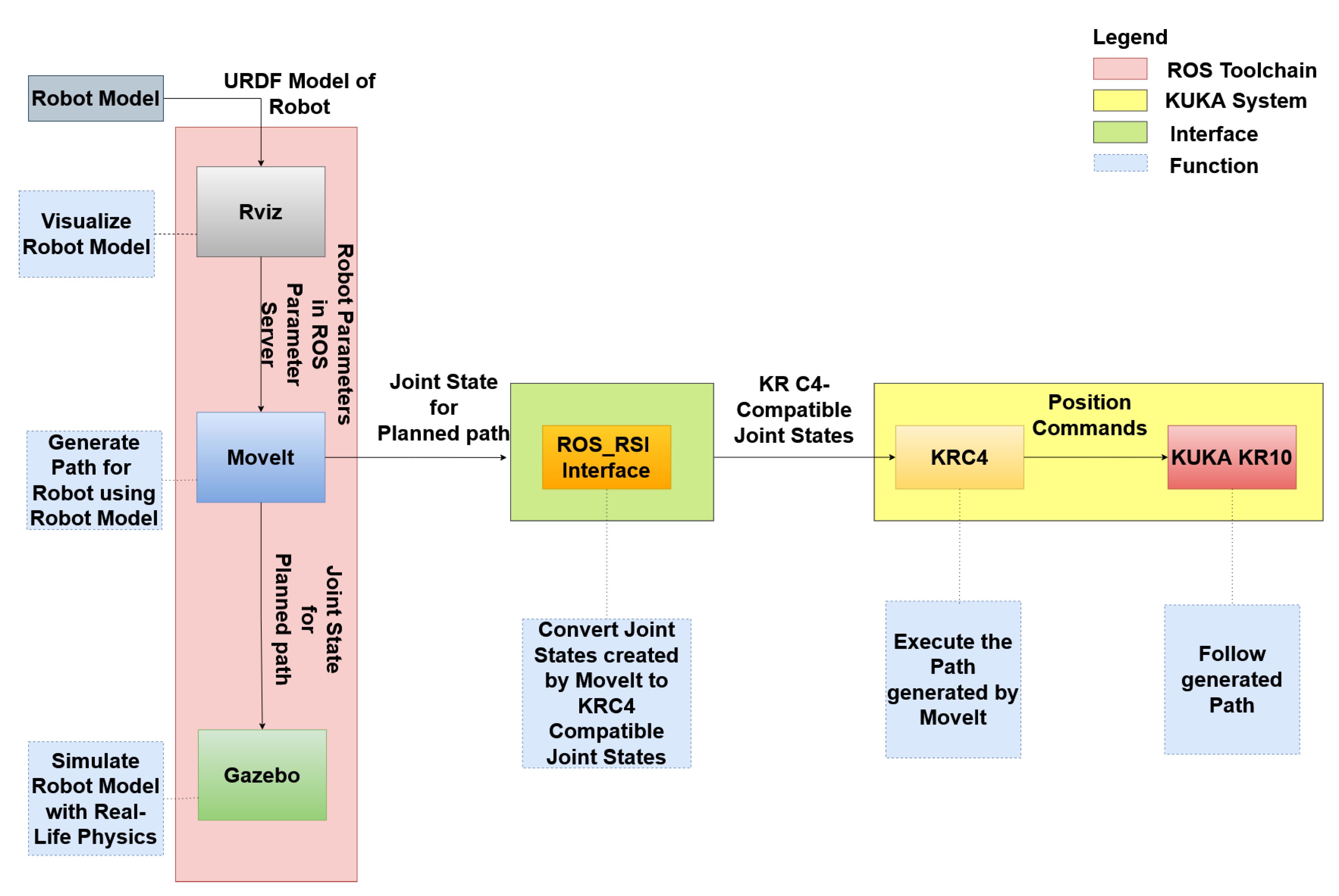
Figure 6 depicts the ROS-based control architecture. The architecture takes the Unified Robot Description Format (URDF) model of the robot as input. URDF is a file format containing information about the serial link of a robotic system and its motion properties, which is used as a primary type in ROS. The visualization of the created model can be conducted using RViz, a visualization tool in the ROS ecosystem. This is the workspace generation step.
The kinematics information contained in the URDF model can then be used by MoveIt! to generate a trajectory between any two poses. MoveIt! is a set of packages and tools for mobile manipulation in ROS that contains state-of-the-art algorithms for motion planning, manipulation, 3D perception, kinematics, collision checking, control and navigation [31]. The generation of the trajectory between the poses is conducted using the Pilz Industrial Motion Planner [32]. For collision checking, the Flexible Collision Library (FCL) is used [33].
Once the trajectory is generated, its execution can be conducted in Gazebo or using the real robot. Gazebo is an open-source 3D simulator for robotics with the ability to simulate real-life sensors and can be used to verify and test robot algorithms in realistic scenarios. This ability can be leveraged to verify the generated path in a simulated environment before executing the path with a physical robot. For the execution of the path using the real robot, the robot-sensor interface (RSI) communication interface provided by KUKA is used. This facilitates the communication between the ROS master and the KUKA KRC4 controller.
RSI is a real-time capable interface between external components and the robot controller. The viewpoint information is sent to the robot by a ROS-node, which takes a list of viewpoints in XML format as an input and converts this data to the KUKA data types and sends it over the ethernet-based RSI interface. The viewpoints sent to the robot via this interface are converted to the according joint angles by the robot controller. In order to acquire data from a measurement system a ROS-node, which subscribes to the topics of the data acquisition system is used. This node stores the data sent from the sensor as soon as the manipulation system has reached its next acquisition pose.
4. Results
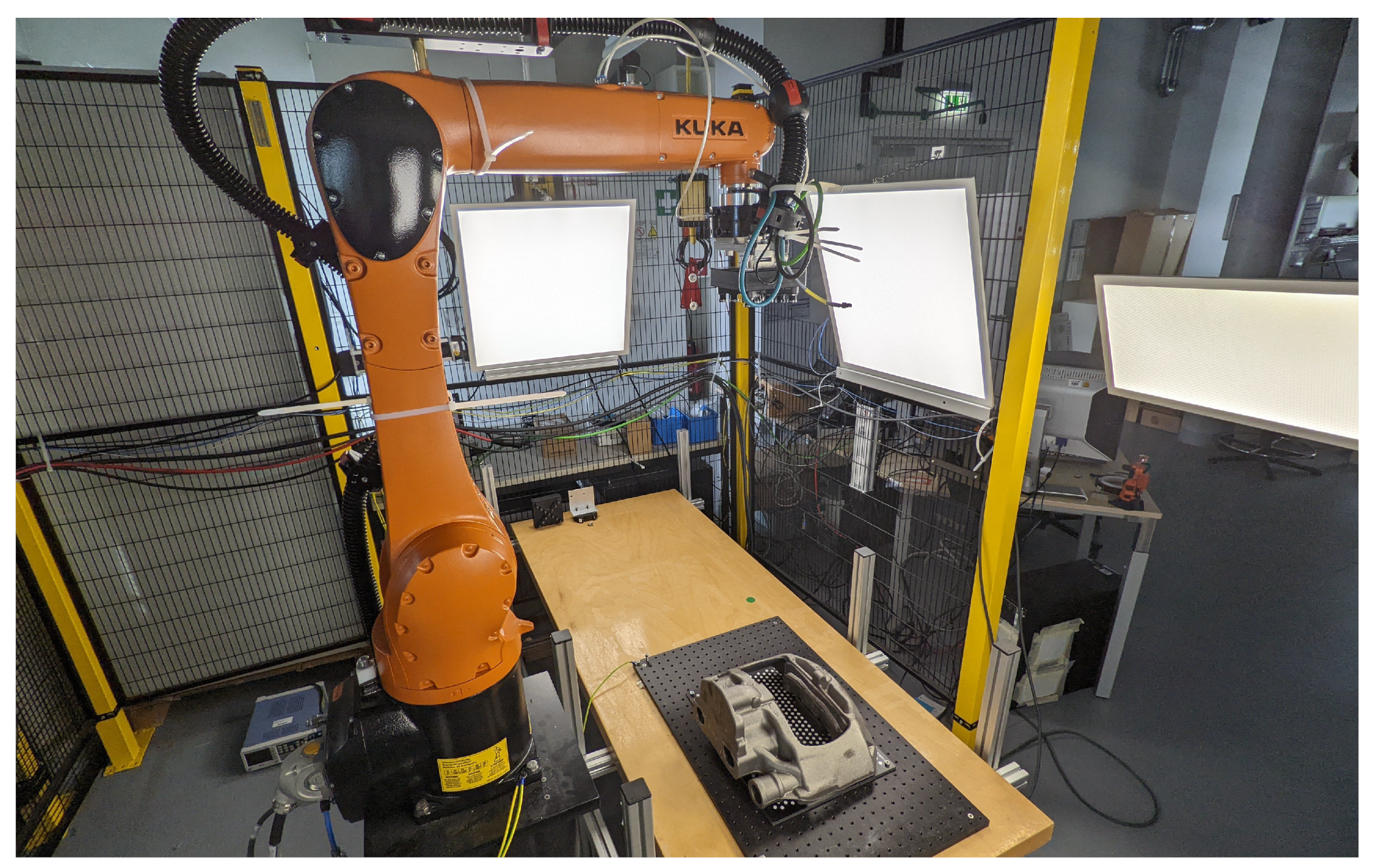
To demonstrate the feasibility and possibilities of the previously described toolchain, it was tested on a sample component. The part to be inspected was a cast automative component with a complex geometry featuring sharp edges, different sized radii and various connected components. The experiments were conducted in a robotic measurement cell consisting of a six-DOF KUKA KR10-R1100 robotic arm with a mounted 3D scanner.
The maximum working radius of this articulated manipulatior is 1100 mm for payloads up to 3 kg. The used scanner was the monochrome stereoscopic Roboception Visard 65 system with a fixed optical focal length of 4 mm. The working distance of the measurement system was set to 500 mm to compare the results obtained with different methods in the processing steps and to provide the best possible depth resolution of the system. Figure 7 depicts the described test environment.
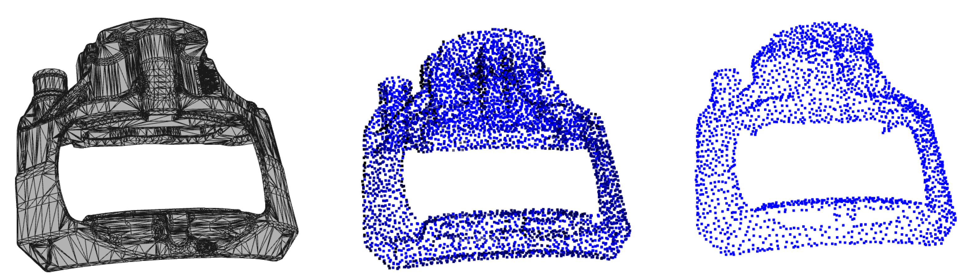
The geometry of the object to be inspected is available in form of a STL model and is shown on the left side of Figure 8. To convert the surface mesh to a point cloud, a uniform point cloud sampling of the STL file was performed. The results are shown in the center of Figure 8. The resulting point cloud has points distributed evenly over the entire surface area.
Due to the layout of the test cell, the object cannot be moved and thus can only be analyzed from one side at a time. The points that are occluded when viewed from the principal inspection hemisphere and thus have to be be removed using the hidden point removal algorithm as described in [34]. The result is shown on the right side of Figure 8. This point cloud is one of the inputs to the toolchain, which was explained in Section 3.
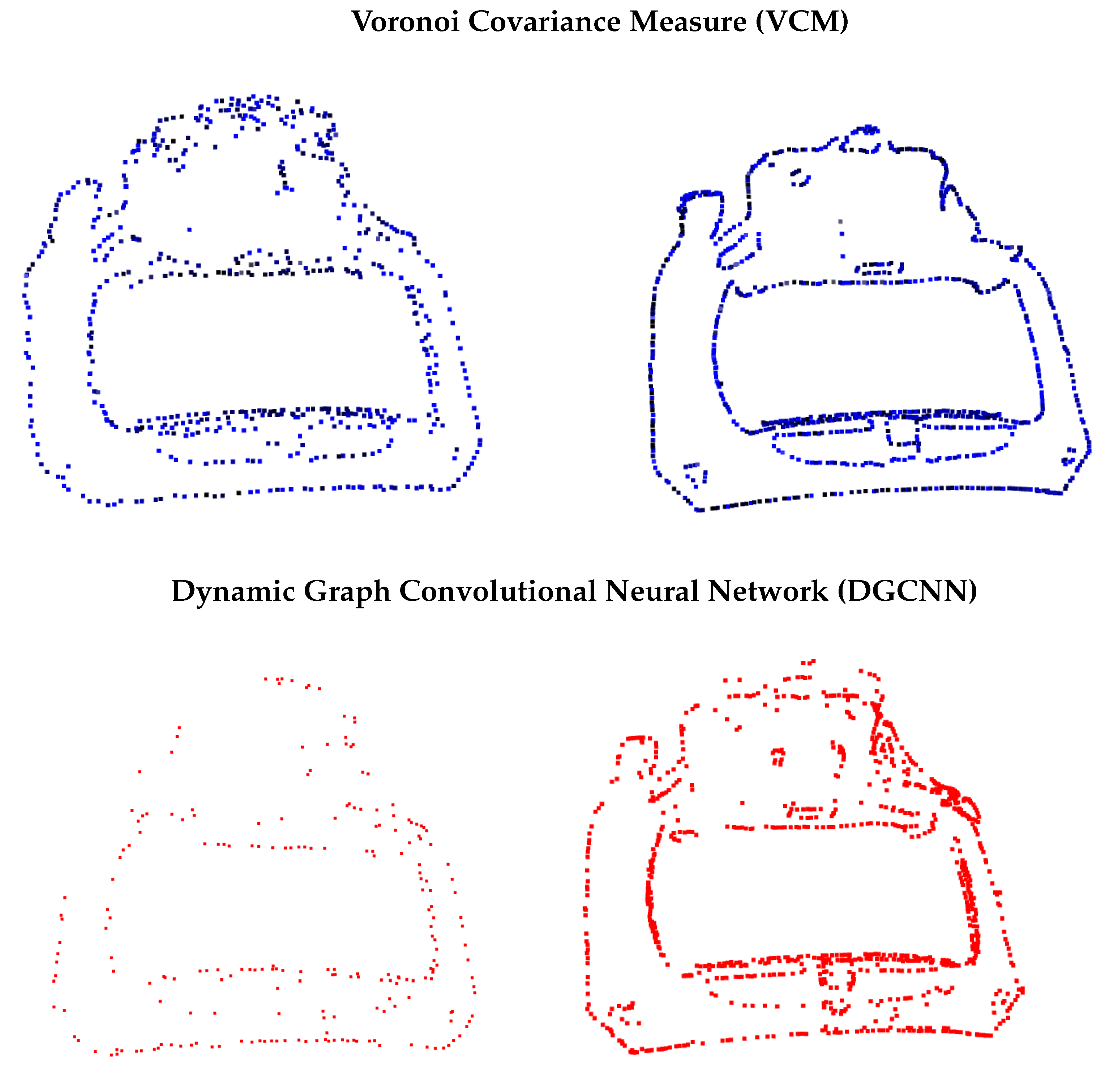
Using this point cloud as input, feature detection was conducted. As mentioned in earlier sections, to demonstrate the flexibility of the designed system, the feature detection step was conducted using two dedicated methods—Voronoi Covariance Measure and Dynamic Graph CNN. To illustrate the relationship between the amount of the points in the input point cloud and the amount of resulting feature points, one sparse and one dense point cloud with 10,000 and 50,000 sample points, respectively, were generated.
The resulting feature points are shown in Figure 9. As expected, the quality of the calculated feature points increases with the density of the point cloud. For the sparse input point cloud of N = 10,000 the VCM algorithm found a satisfying amount of feature points, which can be used for the following segmentation of the object (top left) while the neural network is not able to produce satisfying results for the small number of points (bottom left). For the denser point cloud, the results of both the VCM and DGCNN methods produced comparable and good results (top right and bottom right). However, the computational complexity of both algorithms increased with the number of points in the point cloud. Hence, a good balance between quality of feature detection and computation time must be found.
To ensure comparability between the two methods, the features of the dense point cloud were consequently used to generate the segments using the ToMATo algorithm. For the construction of the Rips complex on the point cloud, the neighborhood parameter was set to a value representing the average dimension of the present feature variations. The initial results of the segmentation step are shown on the left side of Figure 10.
The number of segments correlates directly with the number and density of the detected feature points. The segments show a clear result for the front part of the component but do not segment the back side of the part sufficiently. These initial segments from the ToMATo algorithm are further subdivided using normal-based refinement as required. Clusters are formed taking the mean normal into account and only adding points to a cluster if the differences in the normal direction are below a certain threshold. For this geometry, 21 segments were generated using VCM, and 20 segments were generated using DGCNN as shown on the right side of Figure 10.
Viewpoints were generated for every individual cluster based on the parameters of the used acquisition system. Since the number of viewpoints is very similar for both feature extraction methods, the generated viewpoints were also closely matched. The resulting poses are shown in Figure 11 for the VCM-based clusters (left) and the DGCNN-based clusters (right).
Finally, data could be acquired from the generated viewpoints using the ROS interface of the Roboception 3D scanner. Communication and acquisition were performed using the methods described in Section 3.4. The point clouds hadto be further registered in order to be able to perform analysis operations on them. Once the data was collected from each of the viewpoints, a multi-way registration using the technique presented by Choi [35] was applied. To deal with the noise present in the acquired data a set of filters was applied. The following operations were performed sequentially on the merged data set:
- Plane filtering.
- Statistical outlier removal.
- Nearest-neighbor outlier removal.
Figure 12 shows the results for the VCM- (left) and the DGCNN- (right) based clusters after these operations.
Thus, far, this paper focused on the comparison of the DGCNN- and VCM-based methods for viewpoint generation as two possible methods of the proposed versatile toolchain. In order to evaluate the quality of the reconstructed surfaces, the generated point clouds were compared to a feature ignorant method for viewpoint generation as reference. This reference method used viewpoints on a half-sphere with a radius of 500 mm relative to the center of mass of the inspected part for data acquisition.
Different metrics for the evaluation of point cloud quality exist. Depending on the intended application deviations from a known geometry (CAD matching), geometric features, such as planarity or volume density can be used. In this use case, the volume density, i.e., the number of points in the vicinity of every point of the point cloud, is evaluated for spherical volume elements of radius of 10 mm.
The results are shown in Figure 13 for the two feature-based methods and the reference. The point clouds show similar distributions for both the VCM- and DGCNN-based methods, while the spherical viewpoints resulted in a higher overall density of the part on the top part and it failed to capture the corner areas of the object. This can be seen in the front left and right corners. The feature-based methods thus accomplished a complete scan of the part with a more even density distribution over the entire object. Given the low depth resolution of the Roboception 3D scanner of m, the overall quality of the reconstructed part and the volume density of around 100 points per cm were acceptable.
However, the goal of this work was not to create a system with an optimized accuracy but to show the capabilities of a fully automated and flexible toolchain for component inspection. Future work will focus on the optimization of the methods used in this work and to enhance the overall system performance by the use of a higher resolution measurement system.
5. Discussion
The main goal of this work was to create a flexible toolchain, and the involved processes and components for automated optical 3D metrology tasks were presented. Interchangeability of the specific methods within the toolchain and a high level of adaptibility are the defining features of this system. This was demonstrated by implementing two different feature extraction methods for subsequent viewpoint generation for a digital surface reconstruction of the inspected part.
To achieve this goal, an ontology of inspection processes was derived using the Unified Modeling Language (UML). UML has long been established as the modeling language for ontologies [36]. An ontology was defined as “an explicit specification of conceptualization” in [37] and “can be used to formally model the relevant entities and their relations within a system” [38]. The class/subclass hierarchies, inter-class relationships, class attribute definitions and axioms that specify constraints can easily be represented using UML, which was originally designed for object-oriented programming [36].
As becomes clear from Figure 14, the complexity of a model increases dramatically with the number of components and methods. At the same rate, the interpretability for engineers and researchers to find suitable and successful combinations decreases. However, when used in combination with suitable compilers, ontological models can provide a robust framework for the model-based design of variable systems.
Ontological models along with the design language compiler DC43 have been used successfully to design an extraterrestrial satellite and the engine for a satellite [39,40]. Other ontological models for NDT systems were designed and implemented in [41]. The ontology-based toolchain of Figure 14 should therefore be adoptable to a wide-range of applications provided that suitable interfaces for the connected components are defined.
Future research efforts will be focused on the extension of the presented system. Different measurement systems call for different algorithms for viewpoint generation and data analysis. In order to fully exploit the potential of the ontological model, a design language compiler, such as the Design Cockpit 43, will be used to further evaluate the ROS-based toolchain.
Another aspect of interchangeability is the format of the provided input information to the system. In times of rising individuality of products, the existence of an exact CAD model for the part to be inspected can not always be guaranteed due to the manual post-processing of manufactured parts or automatic adaptations to the product design made by software.
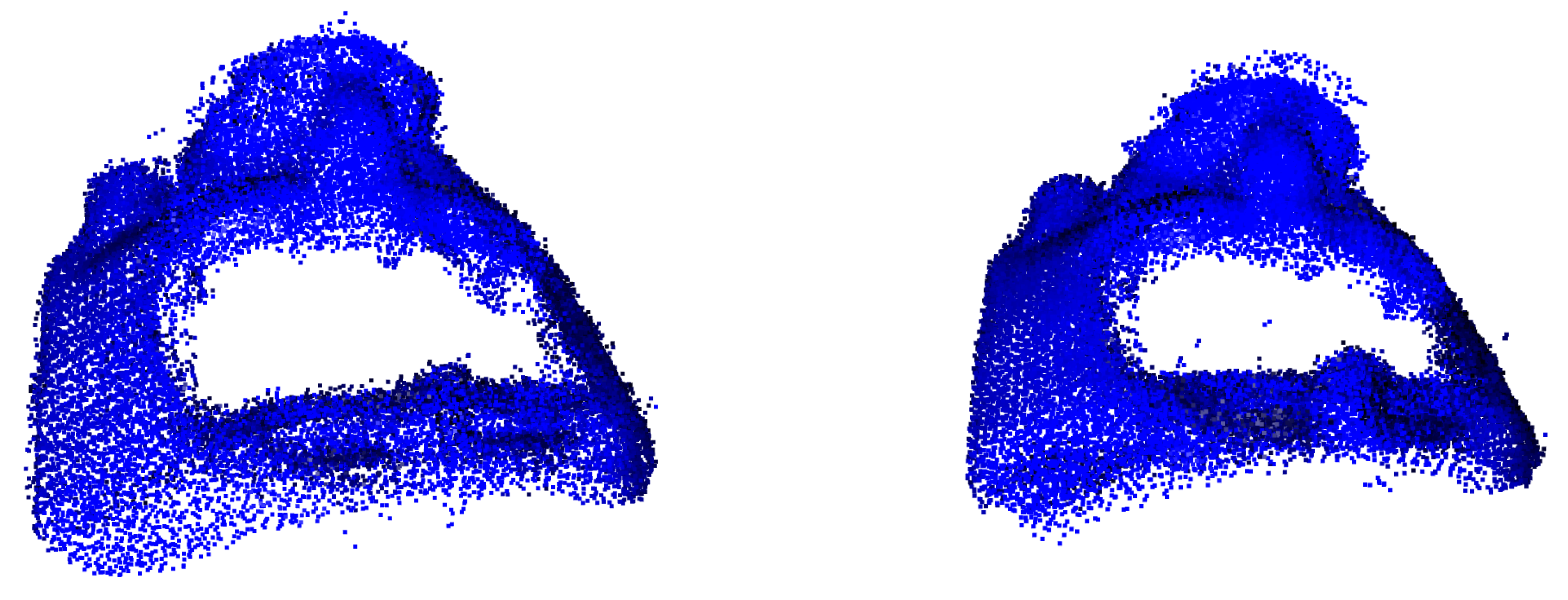
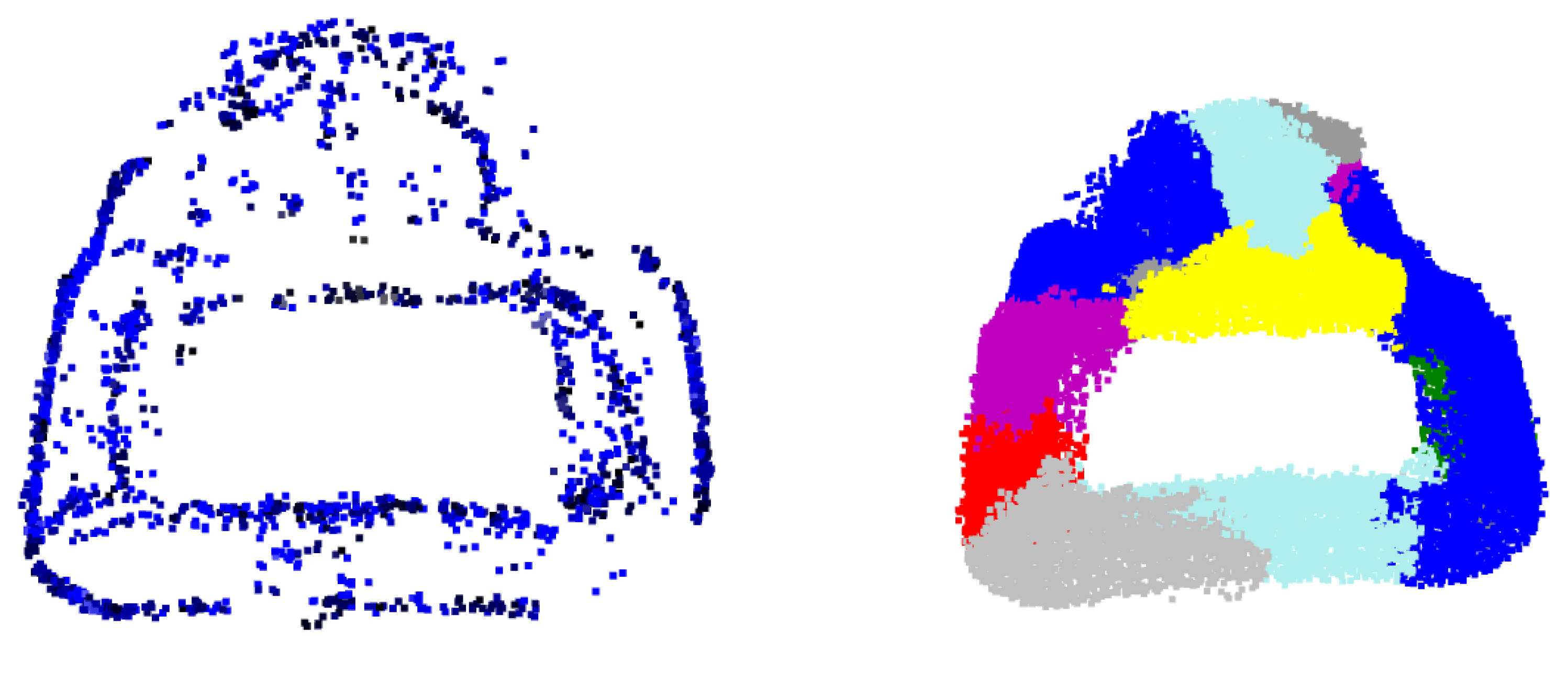
The toolchain can also be used for the inspection of geometries for which reconstructed point cloud data from measurements are available. Using the VCM algorithm for feature point detection and ToMATo algorithm for segmentation, even noisy point cloud data can be processed to reconstruct complex geometries. The results of these operations are shown in Figure 15. The proposed toolchain can thus also be used for the planning of inspection tasks based on low-resolution models created by hand-held or portable measurement systems.
Author Contributions
Conceptualization, P.J., M.E. and F.K.; methodology, P.J., M.E. and F.K.; software, P.J.; validation, P.J., M.E. and F.K.; writing—original draft preparation, P.J. and M.E.; writing—review and editing, P.J., M.E. and F.K.; visualization, P.J. and M.E.. All authors have read and agreed to the published version of the manuscript.
Funding
This research was funded by the German Federal Ministry for Education and Research under grant number 03IHS040.
Data Availability Statement
Restrictions apply to the availability of these data. Data was obtained from Heidelberg Manufacturing GmbH and are available from the authors with the permission of Heidelberg Manufacturing GmbH.
Acknowledgments
The authors would like to thanks the Institute of Materials Resource Management of the University of Augsburg for the possibility of using the Roboception 3D scanners for the experimental studies conducted for this paper.
Conflicts of Interest
The authors declare no conflict of interest.
References
- Stanford Artificial Intelligence Laboratory. Robot Operating System. Available online: https://www.ros.org (accessed on 2 April 2022).
- Bradski, G. The OpenCV Library. Dr. Dobb’S J. Softw. Tools 2000, 25, 120–123. [Google Scholar]
- Rusu, R.B.; Cousins, S. 3D is here: Point Cloud Library (PCL). In Proceedings of the IEEE International Conference on Robotics and Automation (ICRA), Shanghai, China, 9–13 May 2011; IEEE: Shanghai, China, 2011. [Google Scholar]
- Fei, Z.; Zhou, X.; Gao, X.; Zhang, G. A flexible 3D laser scanning system using a robotic arm. Opt. Meas. Syst. Ind. Insp. SPIE 2017, 10329, 1190–1195. [Google Scholar]
- Banerjee, D.; Yu, K.; Aggarwal, G. Robotic arm based 3D reconstruction test automation. IEEE Access 2018, 6, 7206–7213. [Google Scholar] [CrossRef]
- Perez-Cortes, J.C.; Perez, A.J.; Saez-Barona, S.; Guardiola, J.L.; Salvador, I. A System for In-Line 3D Inspection without Hidden Surfaces. Sensors 2018, 18, 2993. [Google Scholar] [CrossRef] [Green Version]
- Wang, J.; Tao, B.; Gong, Z.; Yu, S.; Yin, Z. A mobile robotic measurement system for large-scale complex components based on optical scanning and visual tracking. Robot.-Comput.-Integr. Manuf. 2021, 67, 102010. [Google Scholar] [CrossRef]
- Almadhoun, R.; Taha, T.; Seneviratne, L.; Dias, J.; Cai, G. A survey on inspecting structures using robotic systems. Int. J. Adv. Robot. Syst. 2016, 13, 172988141666366. [Google Scholar] [CrossRef] [Green Version]
- Sølund, T. Towards Plug-n-Play robot guidance: Advanced 3D estimation and pose estimation in Robotic applications. Ph.D. Thesis, Technical University of Denmark, Kongens Lyngby, Denmark, 2016. [Google Scholar]
- Jing, W.; Polden, J.; Tao, P.Y.; Goh, C.F.; Lin, W.; Shimada, K. Model-based coverage motion planning for industrial 3D shape inspection applications. In Proceedings of the 2017 13th IEEE Conference on Automation Science and Engineering (CASE), Xi’an, China, 20–23 August 2017; pp. 1293–1300. [Google Scholar] [CrossRef]
- Szilvśi-Nagy, M.; Mátyási, G. Analysis of STL files. Math. Comput. Model. 2003, 38, 945–960. [Google Scholar] [CrossRef]
- Wu, Q.; Lu, J.; Zou, W.; Xu, D. Path planning for surface inspection on a robot-based scanning system. In Proceedings of the 2015 IEEE International Conference on Mechatronics and Automation (ICMA), Beijing, China, 2–5 August 2015; pp. 2284–2289. [Google Scholar]
- Wu, Q.; Zou, W.; Xu, D. Viewpoint planning for freeform surface inspection using plane structured light scanners. Int. J. Autom. Comput. 2016, 13, 42–52. [Google Scholar] [CrossRef]
- Liu, W.; Ouyang, J.; Qu, X.; Yan, Y. CAD-directed Inspection Planning for Laser Guided Measurement Robot. In Proceedings of the tenth IEEE International Conference on Computer-Aided Design and Computer Graphics, Beijing, China, 15–18 October 2007; pp. 252–257. [Google Scholar] [CrossRef]
- Zou, Q.; Zhao, J. Iso-parametric tool-path planning for point clouds. Comput.-Aided Des. 2013, 45, 1459–1468. [Google Scholar] [CrossRef] [Green Version]
- Zhang, H.; Eastwood, J.; Isa, M.; Sims-Waterhouse, D.; Leach, R.; Piano, S. Optimisation of camera positions for optical coordinate measurement based on visible point analysis. Precis. Eng. 2021, 67, 178–188. [Google Scholar] [CrossRef]
- Ricotta, V.; Mineo, C.; Cerniglia, D.; Reitinger, B. Autonomous 3D geometry reconstruction through robot-manipulated optical sensors. Int. J. Adv. Manuf. Technol. 2021, 116, 1895–1911. [Google Scholar]
- Amenta, N.; Bern, M. Surface reconstruction by Voronoi filtering. Discret. Comput. Geom. 1999, 22, 481–504. [Google Scholar] [CrossRef] [Green Version]
- Alliez, P.; Cohen-Steiner, D.; Tong, Y.; Desbrun, M. Voronoi-based variational reconstruction of unoriented point sets. Symp. Geom. Process. 2007, 7, 39–48. [Google Scholar]
- Mérigot, Q.; Ovsjanikov, M.; Guibas, L.J. Voronoi-based curvature and feature estimation from point clouds. IEEE Trans. Vis. Comput. Graph. 2010, 17, 743–756. [Google Scholar] [CrossRef] [Green Version]
- Qi, C.R.; Su, H.; Mo, K.; Guibas, L.J. Pointnet: Deep learning on point sets for 3d classification and segmentation. In Proceedings of the IEEE Conference on Computer Vision and Pattern Recognition, Honolulu, HI, USA, 21–26 July 2017; pp. 652–660. [Google Scholar]
- Qi, C.R.; Yi, L.; Su, H.; Guibas, L.J. Pointnet++: Deep hierarchical feature learning on point sets in a metric space. Adv. Neural Inf. Process. Syst. 2017, 30, 5105–5114. [Google Scholar]
- Wang, Y.; Sun, Y.; Liu, Z.; Sarma, S.E.; Bronstein, M.M.; Solomon, J.M. Dynamic Graph CNN for Learning on Point Clouds. ACM Trans. Graph. 2019, 38, 146. [Google Scholar] [CrossRef] [Green Version]
- Xing, Z.; Zhao, S.; Guo, W.; Guo, X.; Wang, Y. Processing laser point cloud in fully mechanized mining face based on DGCNN. ISPRS Int. J.-Geo-Inf. 2021, 10, 482. [Google Scholar] [CrossRef]
- Gamal, A.; Wibisono, A.; Wicaksono, S.B.; Abyan, M.A.; Hamid, N.; Wisesa, H.A.; Jatmiko, W.; Ardhianto, R. Automatic LIDAR building segmentation based on DGCNN and euclidean clustering. J. Big Data 2020, 7, 1–18. [Google Scholar] [CrossRef]
- Wang, X.; Xu, Y.; Xu, K.; Tagliasacchi, A.; Zhou, B.; Mahdavi-Amiri, A.; Zhang, H. Pie-net: Parametric inference of point cloud edges. arXiv 2020, arXiv:2007.04883. [Google Scholar]
- Delingette, H. ijcv.final.dvi. Int. J. Comput. Vis. 1999, 32, 111–146. [Google Scholar] [CrossRef]
- Xing, Z.; Zhao, S.; Guo, W.; Guo, X. Geometric feature extraction of point cloud of chemical reactor based on dynamic graph convolution neural network. ACS Omega 2021, 6, 21410–21424. [Google Scholar] [CrossRef] [PubMed]
- Koch, S.; Matveev, A.; Jiang, Z.; Williams, F.; Artemov, A.; Burnaev, E.; Alexa, M.; Zorin, D.; Panozzo, D. ABC: A Big CAD Model Dataset For Geometric Deep Learning. In Proceedings of the IEEE Conference on Computer Vision and Pattern Recognition (CVPR), Long Beach, CA, USA, 15–20 June 2019. [Google Scholar]
- Chazal, F.; Guibas, L.J.; Oudot, S.Y.; Skraba, P. Persistence-based clustering in Riemannian manifolds. JACM 2013, 60, 1–38. [Google Scholar] [CrossRef]
- Chitta, S. MoveIt!: An Introduction. In Robot Operating System (ROS): The Complete Reference (Volume 1); Koubaa, A., Ed.; Springer International Publishing: Cham, Switzerland, 2016; pp. 3–27. [Google Scholar] [CrossRef]
- Pilz GmbH & Co. KG. Motion Blending. 2019. Available online: https://github.com/ros-planning/moveit/blob/master/moveit_planners/pilz_industrial_motion_planner/doc/MotionBlendAlgorithmDescription.pdf (accessed on 5 April 2022).
- Pan, J.; Chitta, S.; Manocha, D. FCL: A general purpose library for collision and proximity queries. In Proceedings of the 2012 IEEE International Conference on Robotics and Automation, Saint Paul, MN, USA, 14–18 May 2012; pp. 3859–3866. [Google Scholar]
- Katz, S.; Tal, A.; Basri, R. Direct visibility of point sets. In ACM SIGGRAPH 2007 Papers; ACM: New York, NY, USA, 2007; p. 24-es. [Google Scholar]
- Choi, S.; Zhou, Q.Y.; Koltun, V. Robust reconstruction of indoor scenes. In Proceedings of the IEEE Conference on Computer Vision and Pattern Recognition, Boston, MA, USA, 7–12 June 2015; pp. 5556–5565. [Google Scholar]
- Kogut, P.; Cranefield, S.; Hart, L.; Dutra, M.; Baclawski, K.; Kokar, M.; Smith, J. UML for ontology development. Knowl. Eng. Rev. 2002, 17, 61–64. [Google Scholar] [CrossRef] [Green Version]
- Gruber, T. A translation approach to portable ontologies. Knowl. Acquis. 1993, 5, 199–220. [Google Scholar] [CrossRef]
- Guarino, N.; Oberle, D.; Staab, S. What is an ontology? In Handbook on Ontologies; Springer: Berlin/Heidelberg, Germany, 2009; pp. 1–17. [Google Scholar]
- Groß, J. Aufbau und Einsatz von Entwurfssprachen zur Auslegung von Satelliten. Ph.D. Thesis, Universität Stuttgart, Stuttgart, Germany, 2014. [Google Scholar]
- Schmidt, J.G.W. Generic Design of Propulsion Systems for Space Systems. Ph.D. Thesis, Universität Stuttgart, Stuttgart, Germany, 2013. [Google Scholar]
- Kamsu-Foguem, B. Knowledge-based support in Non-Destructive Testing for health monitoring of aircraft structures. Adv. Eng. Inform. 2012, 26, 859–869. [Google Scholar] [CrossRef] [Green Version]
Figure 1.
Automated quality inspection can be described as the combination of the three interdependent entities: the (a) Inspected Object, (b) Inspection System and (c) Inspection Task. Each of these entities has its own components and properties.
Figure 1.
Automated quality inspection can be described as the combination of the three interdependent entities: the (a) Inspected Object, (b) Inspection System and (c) Inspection Task. Each of these entities has its own components and properties.

Figure 2.
Toolchain of the Inspection System showing the flow of data from the Inputs to the system and the Processing of this information, to the Execution of the inspection process and the application-specific Evaluation of the results.
Figure 2.
Toolchain of the Inspection System showing the flow of data from the Inputs to the system and the Processing of this information, to the Execution of the inspection process and the application-specific Evaluation of the results.

Figure 3.
Forward and inverse kinematic transformations from joint space to task space and vice versa. A pose in Joint Space is defined by the Joint Angles of the system, while in Task Space, it is defined by Cartesian Coordinates.
Figure 3.
Forward and inverse kinematic transformations from joint space to task space and vice versa. A pose in Joint Space is defined by the Joint Angles of the system, while in Task Space, it is defined by Cartesian Coordinates.
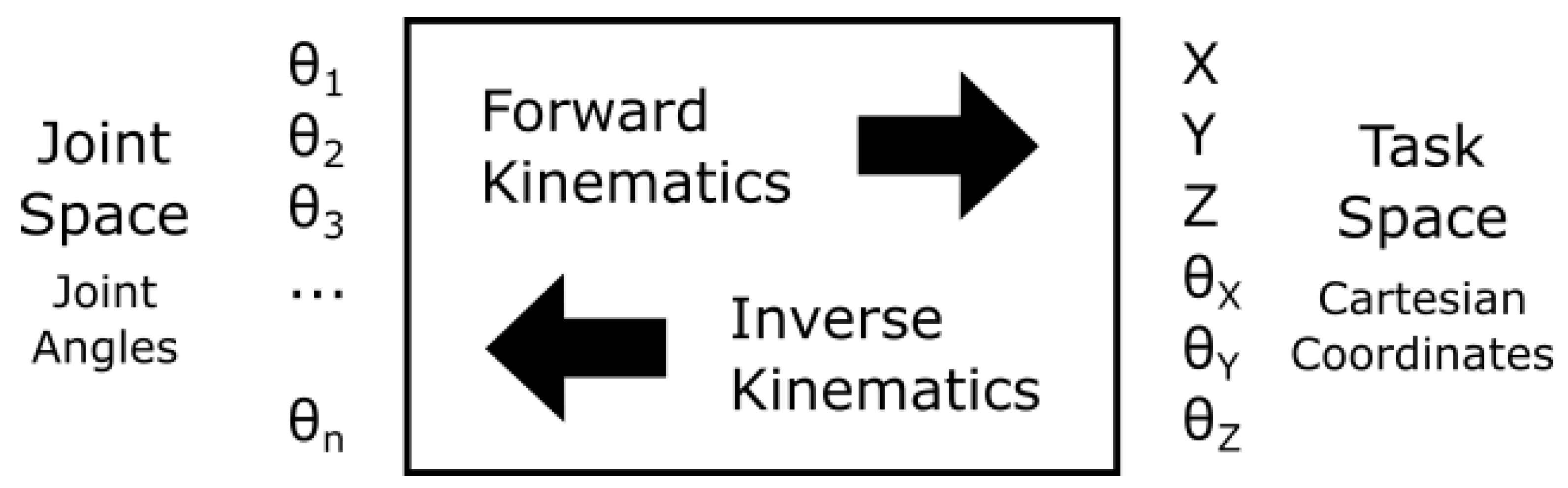
Figure 4.
Architecture of DGCNN-based feature point detector (based on [28]).
Figure 4.
Architecture of DGCNN-based feature point detector (based on [28]).
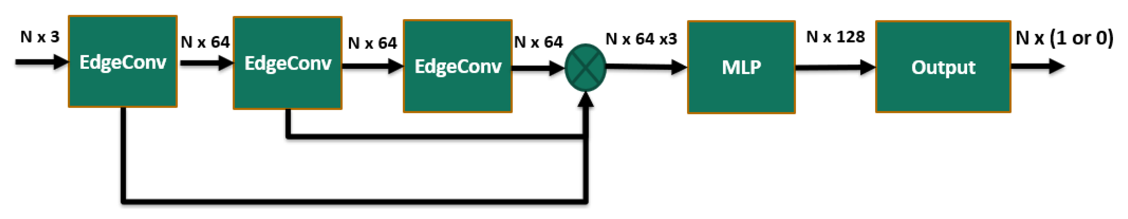
Figure 5.
Projection (left) and viewpoint generation (right).

Figure 6.
ROS-based end-to-end toolchain for automated robot-based inspection tasks.

Figure 7.
Test cell at Fraunhofer IGCV showing the KUKA KR10 robot with a quick change system on the flange, adjustable flicker-free LED panels and threaded grid plate on the inspection table for the flexible positioning of objects.
Figure 7.
Test cell at Fraunhofer IGCV showing the KUKA KR10 robot with a quick change system on the flange, adjustable flicker-free LED panels and threaded grid plate on the inspection table for the flexible positioning of objects.

Figure 8.
Surface mesh model of the component to be analyzed (left), its point cloud representation, (center) and the point cloud after hidden point removal (right).
Figure 8.
Surface mesh model of the component to be analyzed (left), its point cloud representation, (center) and the point cloud after hidden point removal (right).

Figure 9.
Detected feature points using VCM (top left) and DGCNN (bottom right) for a sparse point cloud with 10,000 samples and detected feature points using VCM (bottom left) and DGCNN (bottom right) for a dense point cloud with 50,000 samples.
Figure 9.
Detected feature points using VCM (top left) and DGCNN (bottom right) for a sparse point cloud with 10,000 samples and detected feature points using VCM (bottom left) and DGCNN (bottom right) for a dense point cloud with 50,000 samples.

Figure 10.
The initially generated segments from the detected feature points using VCM (top left) and the segments after normal-based refinement (top right). The generated segments from the detected feature points using DGCNN (bottom left) and the segments after normal refinement (bottom right).
Figure 10.
The initially generated segments from the detected feature points using VCM (top left) and the segments after normal-based refinement (top right). The generated segments from the detected feature points using DGCNN (bottom left) and the segments after normal refinement (bottom right).
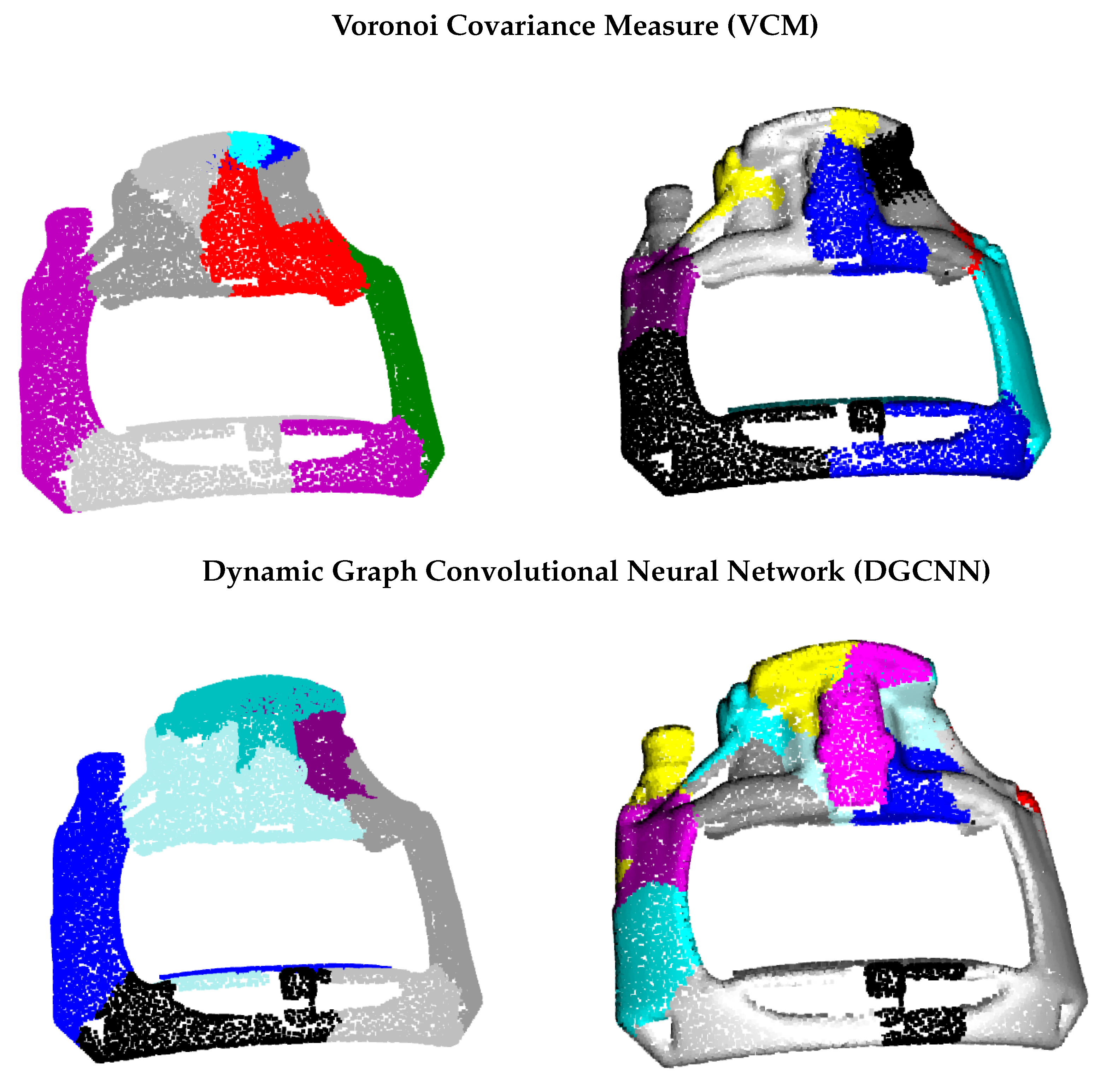
Figure 11.
Generated viewpoints arranged around the test object for the the segments derived from the VCM (left) and DGCNN (right) methods.
Figure 11.
Generated viewpoints arranged around the test object for the the segments derived from the VCM (left) and DGCNN (right) methods.
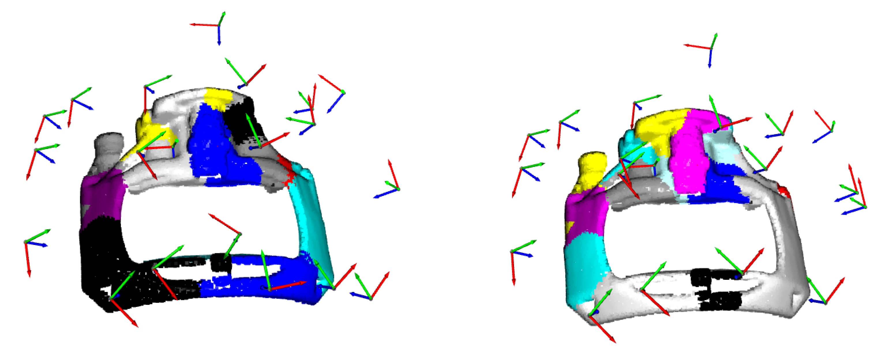
Figure 12.
Reconstructed point cloud using the data collected from viewpoints generated using VCM (left) and DGCNN (right) after filtering of the measurement results.
Figure 12.
Reconstructed point cloud using the data collected from viewpoints generated using VCM (left) and DGCNN (right) after filtering of the measurement results.

Figure 13.
Density of the reconstructed point cloud using VCM (left), DGCNN (center) and spherically arranged viewpoints (right). (%) (100 points per cm as basis).
Figure 13.
Density of the reconstructed point cloud using VCM (left), DGCNN (center) and spherically arranged viewpoints (right). (%) (100 points per cm as basis).
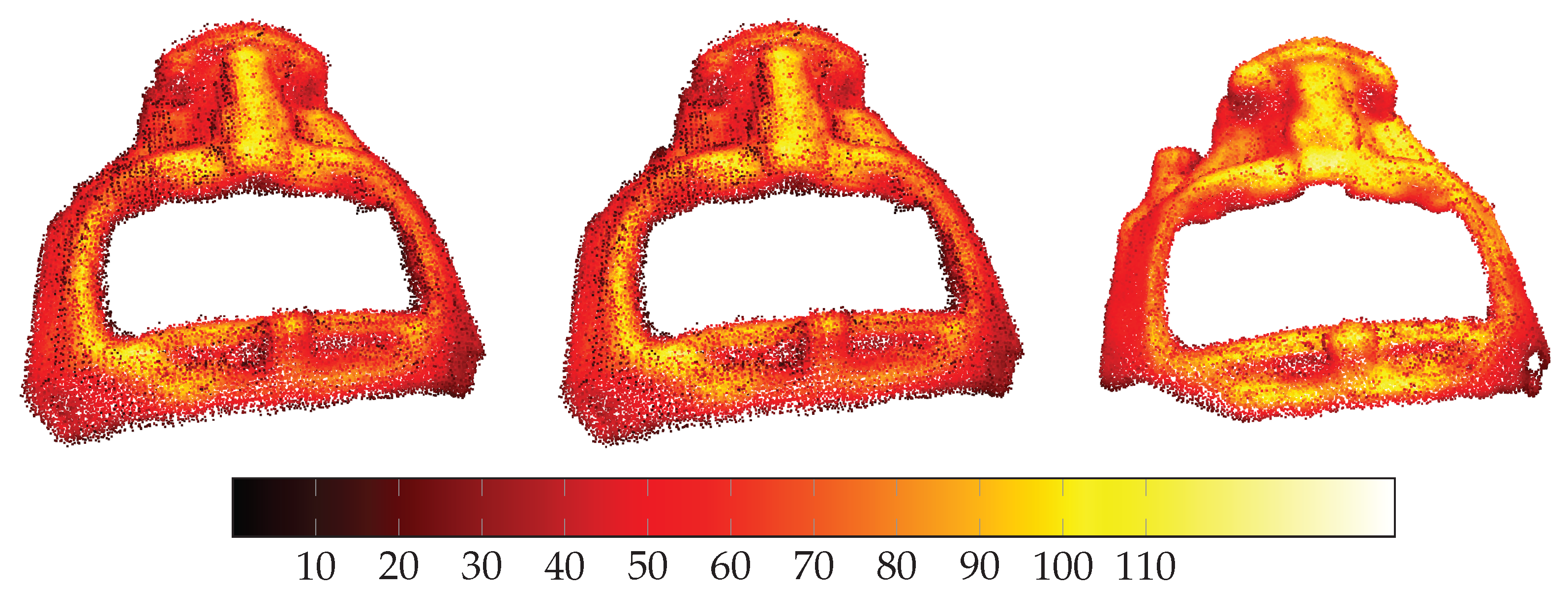
Figure 14.
An overview of the developed extendable system.
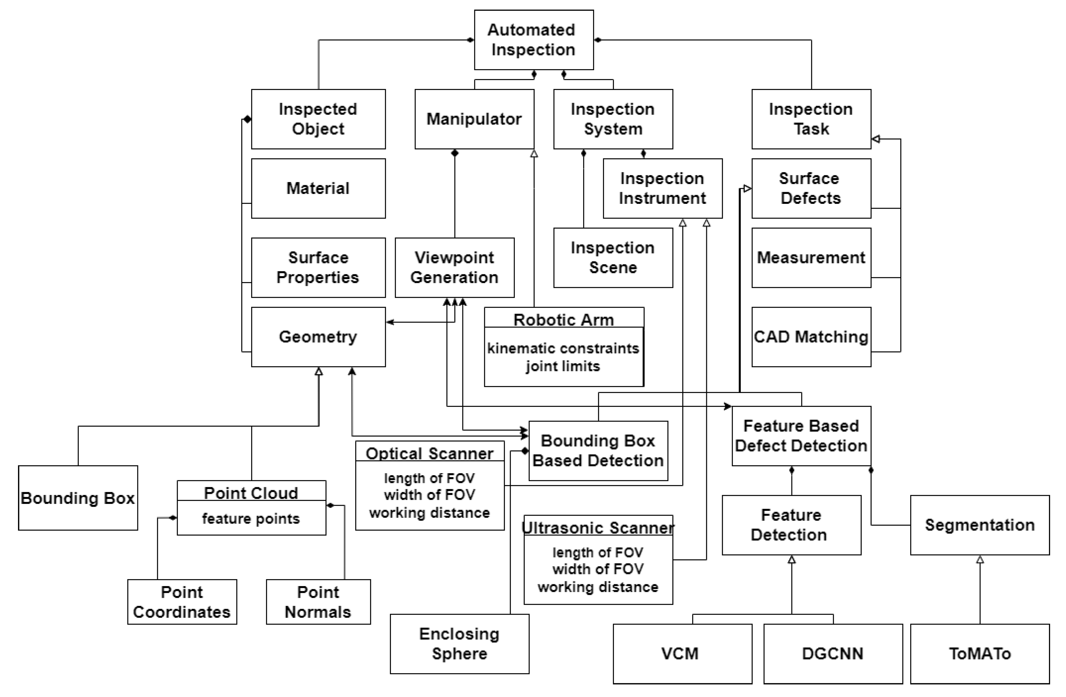
Figure 15.
Feature detection using VCM (left) and segmentation using ToMATo (right) based on a noisy point cloud captured with an optical 3D scanner.
Figure 15.
Feature detection using VCM (left) and segmentation using ToMATo (right) based on a noisy point cloud captured with an optical 3D scanner.
Publisher’s Note: MDPI stays neutral with regard to jurisdictional claims in published maps and institutional affiliations. |
© 2022 by the authors. Licensee MDPI, Basel, Switzerland. This article is an open access article distributed under the terms and conditions of the Creative Commons Attribution (CC BY) license (https://creativecommons.org/licenses/by/4.0/).
Share and Cite
MDPI and ACS Style
Jamakatel, P.; Eberhardt, M.; Kerber, F. Development of a Toolchain for Automated Optical 3D Metrology Tasks. Metrology 2022, 2, 274-292. https://doi.org/10.3390/metrology2020017
AMA Style
Jamakatel P, Eberhardt M, Kerber F. Development of a Toolchain for Automated Optical 3D Metrology Tasks. Metrology. 2022; 2(2):274-292. https://doi.org/10.3390/metrology2020017
Chicago/Turabian StyleJamakatel, Prakash, Maximilian Eberhardt, and Florian Kerber. 2022. "Development of a Toolchain for Automated Optical 3D Metrology Tasks" Metrology 2, no. 2: 274-292. https://doi.org/10.3390/metrology2020017