
A New Stochastic Model for Bus Rapid Transit Scheduling with Uncertainty
by
 , ,
, ,
Milad Dehghani Filabadi
1,* ,
,
Afshin Asadi
2,
Ramin Giahi
3,
Ali Tahanpour Ardakani
4 and
Ali Azadeh
3 1
Department of Management Sciences, University of Waterloo, Waterloo, ON N2L 3G1, Canada
2
Industrial Engineering Department, Sharif University of Technology, Tehran 11365, Iran
3
School of Industrial and Systems Engineering, University of Tehran, Tehran 14170, Iran
4
Department of Data Analytics, Fisher College of Business, The Ohio State University, Columbus, OH 43210, USA
*
Author to whom correspondence should be addressed.
Future Transp. 2022, 2(1), 165-183; https://doi.org/10.3390/futuretransp2010009
Submission received: 29 December 2021
/
Revised: 24 January 2022
/
Accepted: 27 January 2022
/
Published: 6 February 2022
Abstract
:Nowadays, authorities of large cities in the world implement bus rapid transit (BRT) services to alleviate traffic problems caused by the significant development of urban areas. Therefore, a controller is required to control and dispatche buses in such BRT systems.. However, controllers are facing new challenges due to the inherent uncertainties of passenger parameters such as arrival times, demands, alighting fraction as well as running time of vehicles between stops. Such uncertainties may significantly increase the operational cost and the inefficiencies of BRT services. In this paper, we focus on the controller’s perspective and propose a stochastic mixed-integer nonlinear programming (MINLP) model for BRT scheduling to find the optimal departure time of buses under uncertainty. The objective function of the model consists of passenger waiting and traveling time and aims to minimize total time related to passengers at any stop. From the modeling perspective, we propose a new method to generate scenarios for the proposed stochastic MINLP model. Furthermore, from the computational point of view, we implement an outer approximation algorithm to solve the proposed stochastic MINLP model and demonstrate the merits of the proposed solution method in the numerical results. This paper accurately reflect the complexity of BRT scheduling problem and is the first study, to the best of our knowledge, that presents and solves a mixed-integer nonlinear programming model for BRT scheduling.
1. Introduction
Due to increasing environmental pollution and traffic congestion, many strategies on giving some priority to the urban transportation system development have recently been formed. Therefore, bus transit planning captured increasing attention among researchers. A wide area of research is covered by public transit planning and prevention which is divided into a sequence of several distinguished steps, namely (1) route design, (2) setting of frequency, (3) timetabling, (4) vehicle scheduling, (5) crew scheduling, and finally (6) transportation system protection and resilience [1,2,3].
A bus rapid transit system is designed to improve urban mobility and combines the best features of railways with the flexibility and cost advantages of roadway transit. In cities around the world, bus rapid transit (BRT) helps people move more reliably and quickly due to having less congestion with usual traffic because of their dedicated lanes and stations [4]. In ref. [5], the authors represented the advantages of Dar es Salaam BRT which were categorized into economic, social, environmental, political, and urban categories. For example, it has been recently shown that BRT systems have many advantages including affordability, high capacity vehicles, and reliable service [6]. Additionally, ref. [7] introduced some advantages of BRT systems such as alleviating traffic congestion, higher flexibility, better security, user-friendly, etc. In addition to the mentioned advantages, BRT is a flexible, rubber-tired rapid-transit mode that combines vehicles, stations, running ways, fare, ITS, and services component parts into an integrated network with a strong positive identity that provokes an unparalleled prototype [4,5,8,9,10,11,12,13]. It is why BRT has been successfully implemented in many places such as Australia, Iran, South America, and Europe while gaining popularity in North America.
In public transport, the system should meet the demand by providing services to passengers while minimizing one or some objectives such as passengers waiting time, vehicle traveling time, or operational costs (vehicle costs and passenger costs) [2,14]. Static transportation systems were widely studied, e.g., [15,16,17], where parameters of the model are fixed or change periodically given known trends. However, passengers’ parameters such as demand, arrival time, and so on are subject to uncertainty and cannot be predicted by the transportation system controller. Thus, static schedules can lead to inefficiencies, long wait times, and high operational costs that in turn would lead to unreliable transportation systems and a significant drop in using such systems [18,19].
To address data uncertainty and prediction errors, quantitative and predictive approaches have been improved to increase the data collection and prediction precision [20,21,22,23,24]. However, uncertainty is inevitable, and several uncertainty management advancements have been made in recent years. In particular, robust optimization (RO) is an approach to deal with data uncertainty by optimizing for the worst-case scenario. Recent RO studies have shown further advancements in theory, i.e., [25,26], and applications. i.e., [27,28]. Alternatively, stochastic programming (SP) is a branch of mathematical programming to address uncertainty by considering a predefined set of scenarios. SP models occur in most areas of science and engineering from medicine to finance [29] and are less conservative than RO models. In particular, ref. [30] proposed a stochastic model for vehicle scheduling in public bus transport. A more recent extension to SP is the scenario-based approach in which the objective of the scenario-based problems is to find an expected solution that performs under all scenarios. The scenario-based approach has shown applicability benefits in many real-world applications and is easy to deal with in practical situations [31].
Various stochastic-based approaches have been studied in public transportation, especially in BRT scheduling, to cope with fluctuating parameters involved in scheduling the departure time of buses. Among uncertain parameters affecting bus scheduling, most researchers in the last decade proposed approaches where the passengers’ demand for buses is considered unknown and volatile. Particularly, ref. [19] addresses demand uncertainty in BRT using predictive methods and consider the impact of dynamic scheduling on passenger waiting times. Wang et al. [32] developed a data-driven scheme for real-time bus scheduling optimization to minimize the average waiting time of passengers with unknown demand. Kumar et al. [33] dynamically dispatched buses under uncertain demand to minimize the number of trips to maximize the benefit of operators. A recent study by the authors of [34] provided a robust-stochastic model to solve the vehicle scheduling problem, which is extendable to the BRT scheduling problem, with a time window under uncertain demand. An optimization model of the bus departure time and speed scheduling was proposed in [35] to minimize the total waiting time of passengers, subject to uncertain demand. Tang et al. [36] studied the impacts of fluctuating passenger demand on bus scheduling and operational strategies.
Alternatively, researchers have shown that uncertain passenger arrival times can also significantly impact bus scheduling and operational strategies in transportation systems. In particular, a model for the school bus scheduling problem with stochastic travel time was proposed in [37]. In ref. [38], the authors considered stochastic passenger arrival times and proposes a BRT scheduling procedure based on arrival data-based passenger assignment algorithm. Zhang et al. [39] proposed a two-step model of coarse prediction and calibration to predict the passenger flow in real time. The authors of [40] built a stochastic model for BRT scheduling subject to a risk threshold under time-dependent stochastic travel time and ref. [41] proposed a stochastic bus scheduling model with normally distributed travel time and uncertain demand. Li et al. [42] considered uncertain passenger demand and travel time among stops and proposed a timetable optimization model to cope with uncertainties.
The proposed scheduling models are mainly large-scale combinatorial problems that are difficult to solve in polynomial time. The solution methodologies proposed in the literature are mainly categorized into two groups: namely heuristic methods and exact methods. Heuristic algorithms are fast in general and provide a solution that is not necessarily a global optimal solution. Several heuristic-based algorithms such as multi-objective programming, genetic algorithm [43], tabu search [44], simulated annealing [37,45], artificial immune algorithm [46], simulation-based algorithms [47], etc. were employed to solve BRT scheduling problems.
Unlike heuristics, exact methodologies provide a global optimal solution although might be more time-consuming. Due to the practical and computational challenges of such algorithms, they have been less studied in the literature compared to heuristics. In particular, ref. [48] proposed a connection-based network flow or set partitioning algorithm for solving bus scheduling problems. Furthermore, the Lagrangian approach [49] and column-generation strategy [50] have been demonstrated to be effective approaches to solve BRT scheduling considering timetables. However, these methods may not be able to solve all instances and need further investigation.
In this paper, we contribute to the literature of BRT scheduling and present a more comprehensive BRT scheduling model considering uncertainty. In particular, we not only consider the uncertainty in passengers’ demand and arrival time, but we also incorporate stochastic parameters such as (i) running times between stops because these times can be easily impacted by traffic conditions and are not predictable, (ii) passenger traveling time in all stops, because in many developing countries there is not a disciplined program, or even if there is a disciplined program, it may be invoked by several unexpected events such as mismanagement, traffic, passenger immoralities, etc. In this study, we propose a dynamic arithmetic model which can depict the state of the system and correlation for each stochastic parameter during time periods. To more accurately model the problem, we propose a mixed-integer nonlinear programming (MINLP) model aiming to minimize the total operational cost. Furthermore, we implement an outer approximation algorithm to solve the proposed MINLP model for larger instances by providing efficient linear cuts. The main contributions of this paper are highlighted as follows:
- We propose a stochastic MINLP program that more accurately models the characteristics of BRT scheduling problems, especially the cost function.
- The proposed stochastic model considers uncertain parameters to reflect the uncertain nature of transportation systems more accurately. In particular, we consider passenger-related uncertain parameters such as demand, arrival time, the running time between buses, and traveling time.
- We propose an effective scenario-generation method to represent the reality of transportation systems by generating valid representative scenarios for the stochastic model.
- We implement a solution methodology based on an outer approximation (OA) algorithm to effectively solve the proposed MINLP model. We verify the efficiency of the OA algorithm in our numerical example for large enough instances.
The rest of the paper is organized as follows. Section 2 describes the problem. Section 3 introduces the scenario-generation method. Section 4 represents the solution methodology. In Section 5, the computational results are demonstrated. Section 6 discusses the managerial benefits of the proposed approach. Finally, Section 7 concludes the paper.
2. Problem Statement
In this study, we aim to find a solution for buses departure schedules on a one-way route with stops. Running time between stops and passenger’s arrival time into stops are considered as stochastic parameters, and in order to deal with this problem in the real world, some scenarios are generated. The model presented in this paper can be viewed as an extension of the work in [51]. The model in [47] is deterministic where all parameters are assumed to be known in advance. However, the proposed model takes into account uncertain parameters such as running time between stops, the arrival rate of passengers, passengers’ alighting fraction, and so on. Such stochastic programming provides a more realistic model for BRT scheduling that can more efficiently handle inevitable changes in the predicted parameters.
2.1. Assumption
For approaching the reality model, some assumptions are considered as follows:
- Running time between stops is stochastic (i.e., buses do not run at a constant speed, as the running time between stops is uncertain).
- The arrival rate of passengers at stops, passenger alighting fraction in each stop, and passengers’ demand for buses are stochastic.
- The route is a one-way straight line with stops where buses cannot overtake each other.
- The dwelling time of buses at all stops is equal because each bus waits at stops to be loaded to capacity or less. So, dwelling time is almost constant or has extremely slight fluctuations which can be easily ignored, compared to other parameters.
2.2. Notations
Table 1 presents the notations and defines sets, parameters, and decision variables considered in our mathematical model.
2.3. Mathematical Model
The model proposed in the paper can be considered as an extension to that in [51]. So, extending the objective function and adding or altering some constraints and equations are required. The present paper attempts to answer the question of when each bus has to depart from any stop to minimize the total passenger time. The mathematical programming model is presented below:
The objective function of the mathematical model is a combination of the waiting time and traveling time of passengers in all scenarios. The first part of the objective function deals with passengers waiting time which sums the waiting time of all passengers in all stops where both recently arrived passengers and left behind passenger waiting times are taken into consideration. When a bus is loaded to capacity while departing the stop, some passengers cannot board the bus. So, there is an additional waiting time for them, and we assume these passengers wait for the next oncoming bus. The second part of the objective function is passenger traveling time which includes the running time of vehicles between stops and passenger dwelling time at stops. Constraint (2) states that the arrival time of vehicle i at stop k equals its departure time from stop k − 1 plus the running time of the vehicle between these two consecutive stops (i.e., stop k − 1 and k). Constraint (3) shows the number of passengers willing to board vehicle i at stop k is equivalent to the passenger arrival rate multiplied by the headway between two consecutive vehicles plus the number of passengers left behind by vehicle i − 1 at stop k. Constraint (4) states that the number of passengers alight vehicle i at stop k equals to passenger alighting fraction at stop k multiplied by the load in vehicle i departing stop k − 1.
In constraints (5) to (8), the load in bus i departing stop k is restricted. Constraint (5) represents that the load in bus i departing stop k is equal to or less than the demand for bus i at stop k. When bus i at stop k is not at the full capacity (i.e., ), then constraints (5) and (6) are the binding (). Constraint (7) represents that the load in bus i departing stop k is equal to or less than the passenger capacity of the bus. When bus i at stop k is at the full capacity (i.e.,), then constraints (7) and (8) are the bindings (). Constraint (9) shows demand for bus i at stop k which is equal to the load on the bus i departing stop k added to the number of passengers willing to board the bus. In constraint (10), the departure time of bus i at stop k, which is equal to or more than the dwell time of each bus at stops plus the arrival time of bus i at stop k, is restricted. Constraint (11) shows that the departure time of vehicle i at stop k is less than the departure time of vehicle i + 1 at stop k − 1 plus the running time of vehicle i between stop k and k − 1. Constraint (12) shows that the number of passengers left behind at stop k is equivalent to the demand at the same stop for vehicle i less the capacity of bus i. Otherwise, when the capacity of vehicle i is more than the load in bus i departing stop k, then the number of passengers left behind at stop k is equal to zero. Constraint (13) limits to be valued by just 0 or 1, as defined above. Constraint (14), is the non-negativity constraint imposed on the arrival and departure times of buses. Constraint (15) imposes integrality restrictions on integer variables such as the number of passengers willing to board the buses, the number of passengers in buses alighting at stops, passenger capacity of buses, and passengers left behind. The proposed stochastic models (1)–(15) is an MINLP model due to the nonlinear terms and in the objective function (1).
3. Scenario-Generation Method
Most previous models of transportation programming problems are deterministic and assume that parameters are known. However, on the other hand, stochastic models take into consideration parameter uncertainties and represent the real nature of transportation programming more realistically. In stochastic programming, the uncertain parameters are assumed to be known only by their probability distribution functions. In the case of stochastic programming, we confront random parameters with their related continuous distribution functions, while most mathematical models with such parameters cannot be solved, and solution methods need discrete distributions. So, they have to be approximated by a discrete distribution, which in turn limits the number of outcomes into an identical interval [52]. The method in which discrete outcomes are obtained for random variables is called scenario tree generation [53].
A scenario is defined as a set of values for the stochastic variables and is based on a decision tree, in which each path represents a distinct possible scenario and the values assigned to stochastic variables. The number of scenarios exponentially grows with the number of stages. In order to reduce computation cost, some techniques are recommended as follows:
- Replacing stochastic variables by their expected values; therefore, just one scenario is considered.
- Considering the most common scenarios and ignoring the rest.
- Monte Carlo sampling.
- Latin hypercube sampling.
Scenario generation is completely important in terms of reducing computation cost because it just deals with the most common situations. The main scenario-generation methods are sampling, statistical approaches, and simulation.
In this part, we aim to introduce a method for scenario generation for problems dealing with uncertain parameters which in turn can be considered as a cooperation of all methods above. A specific scenario shows the outcomes of all stochastic parameters in a particular event, so for problems with an unlimited number of parameter outcomes, we will confront an infinite number of scenarios that cover all possible consequences. However, studying all these scenarios is not possible and is not even the purpose of problem solvers; they just aim to identify the most common ones. Here we present the steps which are required to generate scenarios, and then a criterion for evaluating scenarios is introduced.
We have proposed certain assumptions for using this method as follows
- Replacing stochastic variables by their expected values; therefore, just one scenario is considered.
- Considering the most common scenarios and ignoring the rest.
- Monte Carlo sampling.
- Latin hypercube sampling.
Here we introduce the steps of the scenario-generation method:
- Finding a well-suited PDF for each stochastic parameter using related historical data.
- Picking out m random values from PDF of each parameter, based on problem requirements.
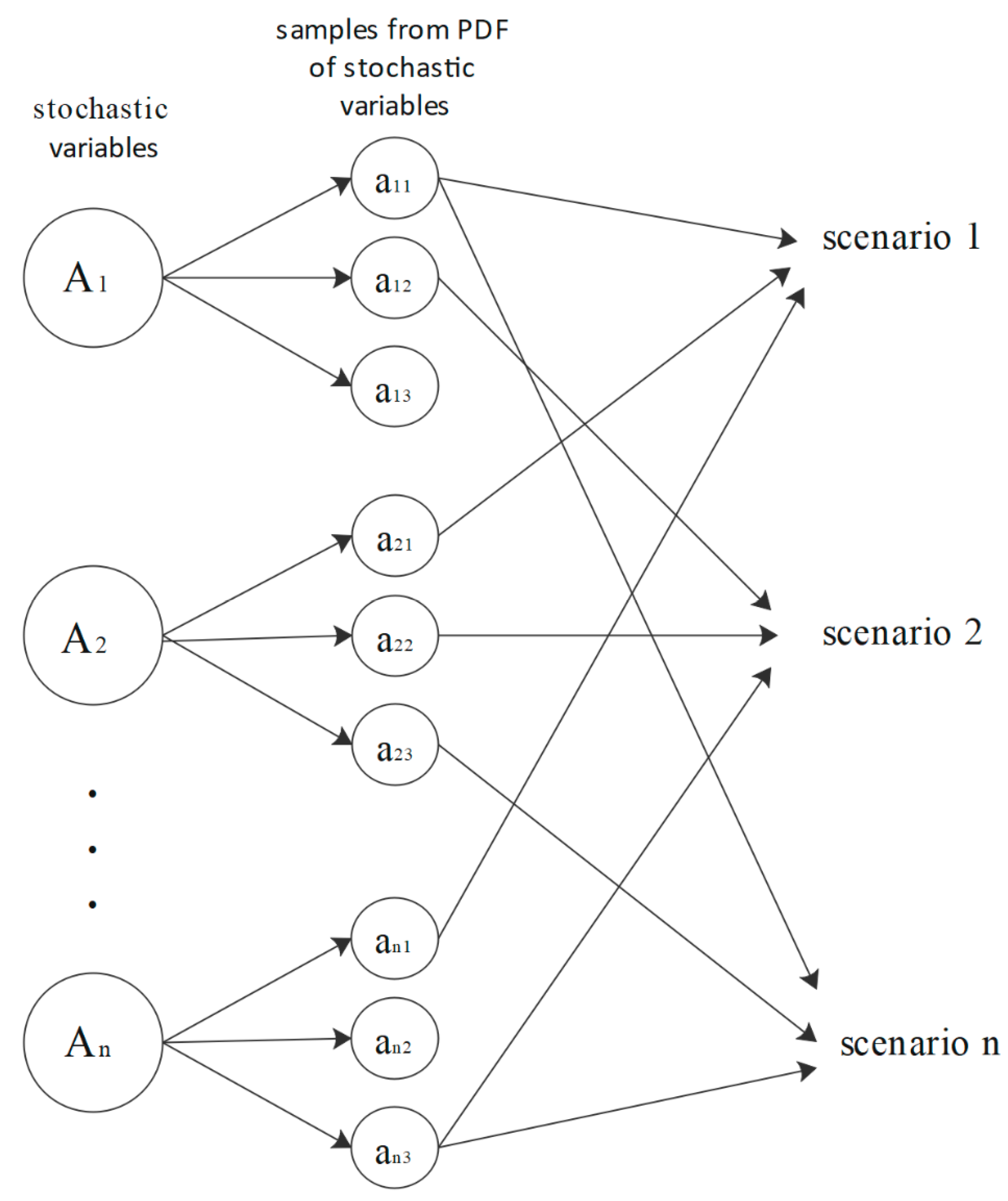
- Every random combination of these samples makes a scenario.
As Figure 1 shows, we can generate as many as samples we need from PDF of stochastic variables. So, an infinite number of scenarios for stochastic problems can be generated. Finding a multi-variable probability distribution function for such problems can be studied in another paper. Here we need to introduce an evaluation criterion for every random scenario made, so we revert to our only knowledge of stochastic parameters, PDF of parameters
Each sample consists of m parameters and we need n stochastic parameter(s) to construct a scenario, so represents sample of stochastic parameter, because in distributions with continuous distribution functions the probability of takes zero value, a symmetric interval of around is defined to calculate the probability for it. So, the g index can be calculated for every single parameter of j. A lower value for the g index of every sample represents that this sample consists of values with higher possibility. Scenarios are a combination of these stochastic parameters, and also an index for every scenario is defined as follows:
The index has this advantage to be considered as a criterion; if a scenario consists of values with higher probability, then the index is lower for that.
Application of Proposed Method in Our Model
To apply the proposed method to generate and evaluate our scenarios, we need to identify our stochastic parameters. In this mathematical model, we deal with three stochastic parameters as follows: passenger demand, passengers’ arrival rate at stops, passengers’ alighting fraction, and running time of buses between stops. Using historical data in Table 2, a well-suited distribution function (considering Anderson–Darling and P-value parameters) for each stochastic parameter can be obtained. These historical data are those presented in [51]. From Table 2, it is observed that passengers’ arrival rate has Lognormal distribution (17) with scale = −1.64466 and location = 0.70687.
Similarly, passengers’ alighting fraction has a lognormal distribution (17) with scale = 0.30014 location = 0.66970.
Running time between stops has a Weibull distribution (19) with shape (k) = 6.65525 and scale (λ) = 3.04438.
Next, we need to provide a sample of 20 random values for every stochastic parameter of the model. So, we randomly generate these samples using the inverse transformation method (ITM) presented in Appendix B.
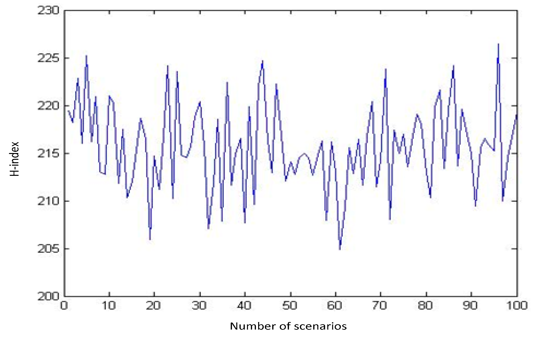
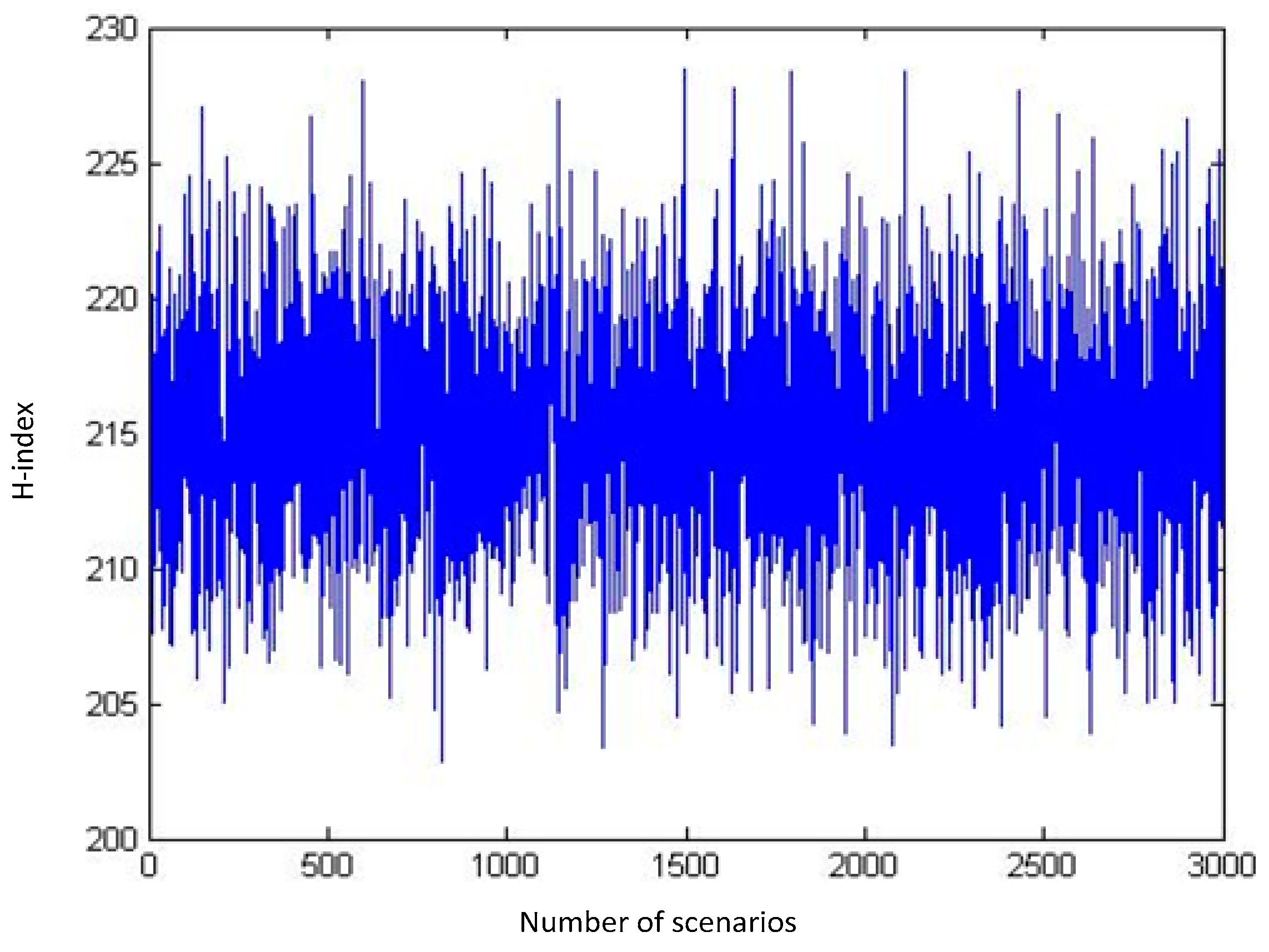
Every combination of these samples makes a scenario. Using MATLAB, we generate numerous scenarios and calculate the H-index for those scenarios. The outputs of our runs for a sequence of 10, 100, 1000, and 3000 distinct random scenarios are shown in Figure 2, Figure 3, Figure 4 and Figure 5 respectively.
It can be inferred from these diagrams that as the number of randomly generated scenarios grows, the H-index tends to follow a normal distribution (Figure 6).
As shown, by changing the number of scenarios from 1000 to 3000 only small changes in Mean and StDev of distribution are caused. So, 1000 scenarios can be enough to fit a normal distribution function for H-indexes. Using a sample of 1000 scenarios, we have fitted a normal distribution for the H-index with a mean of 215 and StDev of 4.009 in our problem as shown in Figure 6. Therefore, as we look for scenarios with the highest possibility to happen, we should go through the scenarios with a lower H-index. Here in our problem, we choose four scenarios with H-indexes in the interval [μ-3σ, μ-2.5σ], which equals to [202.973, 204.97], and with an identical approximation based on the expert judgments and also in order to avoid bias in further analysis, we can consider equal probability for each of these four scenarios. The data for all four scenarios are available in Appendix C.
4. Solution Methodology
Mixed-integer nonlinear programming (MINLP) is a class of optimization problems that consists of (i) linear and nonlinear functions, and (ii) continuous and integer variables. Incorporating integer or binary variables in nonlinear functions makes MINLPs powerful in accurately modeling complex systems. However, it imposes computational challenges on the problem. In particular, the branch and bound (B&B) algorithm that is used for branching on integer variables might be inefficient for such problems since solving MINLP is generally NP-hard. One efficient approach is to add cuts in the B&B method so that the search spaces shrink while the integer solutions are not removed. Among various cutting plane methods proposed in the literature, outer approximation (OA) [54] turns out to be effective in various applications of MINLP [55]. In this section, we implement the OA algorithm in our problem to then verify its efficiency in the numerical results of the next section.
A general MINLP problem can be written as follows:
where functions and are convex and possibly nonlinear. The proposed model in (1)–(15) is a form of problem (20a–d). To clearly show this equivalence, let continuous variable vector be and similarly, integer variable vector be , where bold notation is used for indicating vectors and matrices in problem (1)-(15). Therefore, constraint (20a) corresponds to the objective function (1), constraint (20b) corresponds to the set of constraints (2)–(12), constraint (20c) is a general form of constraint (13) to specify the bounds on integer variables, and finally, constraint (20d) corresponds to the set of constraints (14) and (15). For brevity and simplicity in notations, we show the steps of the OA algorithm on the general problem (20a) in matrix form. Then in our implementation, we use the proper definitions of variable vectors and and also functions and to map problem (1)–(15) to problem (20a–d). The idea of the OA algorithm is to effectively exploit the structure of the original problem based on principles of decomposition. So, the OA solves a series of mixed-integer linear programs (MILP) and a set of nonlinear programs (NLP), sequentially [54], and consists of two steps, namely the subproblem and master problem.
4.1. Subproblem (SP)
The subproblem initially fixes the integer variables and then solves an NLP for given integer variables. Generally, the subproblem at iteration can be written as a nonlinear program (21a–c) where is the fixed values of integer variables.
Subproblem (21a–c) finds the optimal solution for fixed , and since we solve this problem iteratively, we denote optimal solution by . Term of subproblem (21a–c) provides an upper bound on the optimal value of z in the original problem (20a–d). It is because we restricted the integer values to take fixed values, and adding restrictions shrinks the feasible region, which in turn might increase the objective function value or keep it unchanged. Thus,
4.2. Master Problem (MP)
Once the solution of the continuous variable in iteration is known, i.e., , the master problem uses the value of to outer approximate the nonlinear function at this point by generating a cut. The master problem solves a MILP where the nonlinear functions are linearized. The master problem (22a–e) is shown as follows.
Constraints (22b,c) correspond to the cuts to linearize (outer approximate) nonlinear functions. Since in (22b) we approximated the nonlinear function from below, the master problem provides a lower bound on the objective function value of the original problem (20a–d). The OA algorithm can terminate based on a prespecified condition. In particular, one efficient stopping condition is to check the gap between the upper and lower bounds on the original objective function value, i.e., . Once is within an acceptable value , which is defined by the user, we can terminate the algorithm, as shown in Figure 7. Further details on the implementation of the OA algorithm can be found in [54,55,56].
5. Computational Results
In this section, we numerically demonstrate the performance of the proposed model. First, we provide a numerical example for a one-way route with 15 buses operating and 20 stops. This instance is solved using BARON, presented in Appendix A, to obtain the departure time of all buses. Then, to verify the performance of the OA algorithm, we consider larger instances and compare the computational time of BARON and OA algorithms for the proposed stochastic MINLP model. All instances are solved in GAMS 22.8 on a 2.5 GHz, 2 GB of RAM memory.
5.1. Demonstrative Example
To demonstrate the performance of the proposed model, we consider a one-way route with 20 stops that are sequentially located on the route and are numbered in order. For instance, the first stop is stop #1 and the last stop is stop #20. Additionally, we consider 15 operating buses that stop at all designated stops to pick up and drop off passengers and then complete their trip when they reach stop #20. Given the scenarios generation method, we generate a number of scenarios, out of which four scenarios are the most representative ones that are considered in the model. Details of these four scenarios are available in Appendix C. The departure time of buses from stop one is shown in Table 3.
To validate the proposed stochastic model, we should demonstrate whether this approach can be optimal or not. In order to answer this issue, two concepts are provided: the expected value of perfect information (EVPI), and the value of the stochastic solution (VSS). Here, we only use EVPI which measures the maximum amount of payment that is paid by a decision-maker for accurate and complete information about the future. VSS assesses the value of using distributions on future results [57].
EVPI = RP − WS
In the RP (resource problem), the objective function is solved by considering all scenarios. In the WS (wait and see solution) approach, the objective function is independently solved in each scenario, and then the mean of the objective function is considered as WS. The RP, WS, and EVPI of the objective function are shown in Table 4. The zero value for the EVPI index numerically demonstrates the validity of the proposed stochastic model and it is due to properly addressing uncertain parameters in the proposed model.
5.2. Computational Results
In this section, we demonstrate the performance of the OA algorithm by providing comparisons with the BARON solver. We consider 10 randomly generated test cases, with five instances for each case, and vary the number of buses (B) and the number of stops (S) in test cases. For each test case, we follow the same scenario-generation method explained in Section 3. The proposed OA algorithm is terminated once one of the following criteria is attained: (i) master problem (22a–e) is infeasible; (ii) maximum iteration is larger than 50; (iii) the gap is less than or equal to 1%; (iv) computing time reaches 1800 s.
Table 5 compares the computational performance of the OA algorithm and BARON solver, where each test case is solved five times using each algorithm. The sixth and ninth columns labeled “ratio” correspond to the percentage of instances that are solved to global optimal within the time limit of 1800 s.
From Table 5, it is observed that both the OA algorithm and BARON solver are able to handle instances with a low number of buses and stops (small-scale test cases). In such cases (test cases 1, 2, and 3), the BARON solver is slightly better. It is because the cuts that are generated in the OA algorithm are not very effective in such cases. However, as the instances get larger, the OA algorithm outperforms the BARON solver. For instance, in test case 8 OA algorithm can find the global optimal solution in all instances. However, none of the five random instances can be solved to global optimality using BARON solver within 1800 s. Such results show how many computational improvements we can make if the OA algorithm is efficiently implemented in the BRT scheduling problem. Although OA is efficient, test case 10 cannot be solved using OA within the time limit. This suggests researchers propose more advanced solution method procedures for solving such problems.
6. Discussion: Managerial Benefits of the Proposed Approach
Traffic controllers and managers are constantly looking for potential frameworks that can cope with various challenges in planning and scheduling buses in transportation systems. Most challenges come from the unpredictability of passenger’s behavior such as their arrival time, demand, and so on. In this research, we have proposed a new stochastic model to deal with such uncertainties and provide an efficient way of scheduling buses in BRT systems. From a managerial point of view, the proposed model allows managers to prepare for uncertain events in BRT systems and provide a better understanding of the different impacts that passengers’ data variation can cause an increase in the operational costs. The proposed model help managers make decisions about short-term and long-term plans, relevant policies, and strategies in a BRT system. For instance, in a highly uncertain BRT system, managers can use the output of the model to identify and prioritize possible actions such as increasing the number of buses, assigning special lanes for buses, or setting preventive policies to decrease traveling time uncertainties. As a practical merit of the proposed model, managers can use the historical data, and based on the level of uncertainty in the past data, they can determine a finite set of scenarios to be considered in the model so that the optimal schedule meets the system requirements under all scenarios. Furthermore, the solution methodology implemented in this research provides useful insights about the size and complexity of the problem to consider. In particular, using the commercial solvers, one can schedule the buses in a smaller BRT system. However, this research helps managers know the computational limits of the proposed model and guide them to choose a proper solution methodology. Therefore, users can use the computational results to decide the size of the BRT system they would like to consider without running into computational issues.
7. Conclusions
Considering the uncertainty of transit systems due to traffic conditions and so on, models dealing with stochastic parameters, which are closer to real situations, are required. In this study, a scenario-based stochastic programming model is proposed. In this model, the objective function consists of two parts. The first and the second parts deal with passenger waiting times and passenger traveling times, respectively, in order to minimize the total related time of passengers. Then, a new method for generating the scenarios is presented, which generates four scenarios representing the most common states in our numerical example. This paper also implemented an outer approximation algorithm to solve the proposed stochastic MINLP algorithm more efficiently and discussed the merits and limitations of the OA algorithm. It turns out that the OA algorithm is efficient for larger instances. However, once the test cases get significantly large, OA reaches its limitations. Therefore, a future research direction is to combine the OA algorithm with other cutting algorithms to advance the solution methodologies in BRT scheduling problems.
Author Contributions
Conceptualization, A.A. (Afshin Asadi) and R.G.; methodology, M.D.F.; software, M.D.F., A.A. (Afshin Asadi) and A.T.A.; validation, M.D.F., A.A. (Afshin Asadi) and R.G.; formal analysis, M.D.F., A.A. (Afshin Asadi), R.G. and A.T.A.; investigation, M.D.F., A.A. (Afshin Asadi) and R.G.; resources, A.A. (Ali Azadeh); data curation, A.A. (Afshin Asadi), R.G. and A.T.A.; writing—original draft preparation, A.A. (Afshin Asadi) and A.A. (Ali Azadeh).; writing—review and editing, M.D.F.; visualization, M.D.F., A.A. (Afshin Asadi), R.G. and A.T.A.; supervision, M.D.F. and A.A. (Ali Azadeh); project administration, M.D.F. All authors have read and agreed to the published version of the manuscript.
Funding
This research received no external funding.
Institutional Review Board Statement
Not applicable.
Informed Consent Statement
Not applicable.
Data Availability Statement
Not applicable.
Conflicts of Interest
The authors declare no conflict of interest.
Appendix A
The Branch-And-Reduce Optimization Navigator (BARON) is a GAMS solver for the global solution of nonlinear programs (NLP), and also mixed-integer nonlinear programs (MINLP). While traditional NLP and MINLP algorithms are guaranteed to converge merely under certain assumptions of convexity, algorithms of deterministic global optimization of the branch-and-bound type which are guaranteed to provide global optima under fairly general assumptions are implemented by BARON. These include the existence of finite upper and lower bounds on nonlinear expressions in the NLP or MINLP to be solved.
Appendix B
Random variable generation using the inverse transformation method (ITM): Suppose that we have a distribution function of random variable x as f(x). Its cumulative distribution function (F(x)) can be obtained. The values for x distributed according to f(x) are gained through these steps:
- Generate u~U [0, 1]
- Let
- Then ,
- Proof:
Appendix C
The data used for all four scenarios are presented here.

Table A1.
Values of stochastic parameters in scenario one.
| Stops | Passenger Alighting Fraction | Passenger Arrival Rate | Running Time between Stops |
|---|---|---|---|
| 1 | 0.02 | 1.3 | - |
| 2 | 0.41 | 2.2 | 192 |
| 3 | 0.09 | 4.1 | 150 |
| 4 | 0.13 | 2.1 | 210 |
| 5 | 0.31 | 2.5 | 174 |
| 6 | 0.3 | 2.7 | 282 |
| 7 | 0.13 | 2.3 | 168 |
| 8 | 0.06 | 2.6 | 138 |
| 9 | 0.25 | 2.4 | 120 |
| 10 | 0.08 | 1.1 | 150 |
| 11 | 0.67 | 2.3 | 390 |
| 12 | 0.06 | 3.2 | 174 |
| 13 | 0.14 | 1.9 | 132 |
| 14 | 0.81 | 1.2 | 120 |
| 15 | 0.11 | 1.3 | 216 |
| 16 | 0.17 | 2.8 | 288 |
| 17 | 0.1 | 2.6 | 222 |
| 18 | 0.37 | 2.4 | 180 |
| 19 | 0.15 | 1.7 | 366 |
| 20 | 0.2 | 2.9 | 216 |
Table A2.
Values of stochastic parameters in scenario two.
| Stops | Passenger Alighting Fraction | Passenger Arrival Rate | Running Time between Stops |
|---|---|---|---|
| 1 | 0.24 | 1.1 | - |
| 2 | 0.04 | 3.3 | 156 |
| 3 | 0.1 | 2.4 | 282 |
| 4 | 0.41 | 2 | 204 |
| 5 | 0.09 | 3.2 | 126 |
| 6 | 0.03 | 2.9 | 240 |
| 7 | 0.41 | 3.5 | 222 |
| 8 | 0.46 | 3.9 | 156 |
| 9 | 0.49 | 1.1 | 222 |
| 10 | 0.02 | 2.2 | 186 |
| 11 | 0.84 | 2.1 | 150 |
| 12 | 0.13 | 0.6 | 120 |
| 13 | 0.42 | 2.2 | 156 |
| 14 | 0.17 | 2.4 | 264 |
| 15 | 0.15 | 0.5 | 180 |
| 16 | 0.19 | 2.2 | 162 |
| 17 | 0.04 | 2.1 | 168 |
| 18 | 0.21 | 1 | 174 |
| 19 | 0.09 | 1.9 | 210 |
| 20 | 0.12 | 0.9 | 240 |
Table A3.
Values of stochastic parameters in scenario three.
| Stops | Passenger Alighting Fraction | Passenger Arrival Rate | Running Time between Stops |
|---|---|---|---|
| 1 | 0.18 | 1.7 | - |
| 2 | 0.42 | 2.4 | 144 |
| 3 | 0.35 | 2.4 | 402 |
| 4 | 0.15 | 1.2 | 234 |
| 5 | 0.4 | 3.4 | 180 |
| 6 | 0.59 | 2.2 | 144 |
| 7 | 0.08 | 2.6 | 426 |
| 8 | 0.06 | 2.3 | 414 |
| 9 | 0.28 | 3.3 | 198 |
| 10 | 0.3 | 1.3 | 258 |
| 11 | 0.34 | 2.6 | 126 |
| 12 | 0.03 | 1.4 | 204 |
| 13 | 0.01 | 2 | 162 |
| 14 | 0.18 | 3 | 120 |
| 15 | 0.16 | 1.9 | 180 |
| 16 | 0.64 | 2.8 | 180 |
| 17 | 0.1 | 2 | 228 |
| 18 | 0.24 | 2.6 | 306 |
| 19 | 0.07 | 2.4 | 156 |
| 20 | 0.06 | 2 | 132 |
Table A4.
Values of stochastic parameters in scenario four.
| Stops | Passenger Alighting Fraction | Passenger Arrival Rate | Running Time between Stops |
|---|---|---|---|
| 1 | 0.12 | 1 | - |
| 2 | 0.6 | 3 | 168 |
| 3 | 0.13 | 1.8 | 174 |
| 4 | 0.27 | 2.4 | 138 |
| 5 | 0.12 | 3.4 | 132 |
| 6 | 0.44 | 1.2 | 132 |
| 7 | 0.37 | 2 | 186 |
| 8 | 0.66 | 0.8 | 132 |
| 9 | 0.08 | 1.9 | 138 |
| 10 | 0.58 | 1.1 | 126 |
| 11 | 0.1 | 1.7 | 240 |
| 12 | 0.49 | 1.6 | 198 |
| 13 | 0.3 | 2 | 138 |
| 14 | 0.04 | 1.9 | 144 |
| 15 | 0.58 | 2.6 | 156 |
| 16 | 0.31 | 1.4 | 162 |
| 17 | 0.67 | 2.2 | 126 |
| 18 | 0.13 | 3.6 | 126 |
| 19 | 0.12 | 1.7 | 120 |
| 20 | 0.21 | 2.6 | 120 |
References
- Filabadi, M.D.; Bagheri, P. Robust-and-Cheap Framework for Network Resilience: A Novel Mixed-Integer Formulation and Solution Method. arXiv 2021, arXiv:211009694. [Google Scholar]
- Guihaire, V.; Hao, J.-K. Transit network design and scheduling: A global review. Transp. Res. Part A Policy Prac. 2008, 42, 1251–1273. [Google Scholar] [CrossRef] [Green Version]
- Arabi, M.; Hyun, K.K.; Mattingly, S. Adaptable Resilience Assessment Framework to Evaluate an Impact of a Disruptive Event on Freight Operations. Transp. Res. Rec. 2021, 2675, 1327–1344. [Google Scholar] [CrossRef]
- Cui, X.; Zhuang, S.; Gao, J. Systemic Research of Bus Rapid Transportation. In Proceedings of the 2010 3rd International Conference on Information Management, Innovation Management and Industrial Engineering, Kunming, China, 26–28 November 2010; Volume 2, pp. 332–335. [Google Scholar]
- Mzee, P.K.; Chen, Y. Notice of Retraction: Implementation of BRT system in developing countries as the best option in reducing emission the case study of dart system in Dar es Salaam. In Proceedings of the 2010 IEEE International Conference on Advanced Management Science (ICAMS 2010), Chengdu, China, 9–11 July 2010; Volume 2, pp. 532–537. [Google Scholar]
- Li, F.; Duan, Z.; Yang, D. Dwell time estimation models for bus rapid transit stations. J. Mod. Transp. 2012, 20, 168–177. [Google Scholar] [CrossRef] [Green Version]
- Dong, X.; Xiong, G.; Fan, D.; Zhu, F.; Lv, Y. Research on bus rapid transit (BRT) and its real-time scheduling. In Proceedings of the 2011 IEEE International Conference on Service Operations, Logistics and Informatics, Beijing, China, 10–12 July 2011; pp. 342–346. [Google Scholar]
- Chuanjiao, S.U.N.; Wei, Z.; Yuanqing, W. Scheduling combination and headway optimization of bus rapid transit. J. Transp. Syst. Eng. Inf. Technol. 2008, 8, 61–67. [Google Scholar]
- Ding, H.; Guoqiang, Y.; Yuan, M. Study of Bus Rapid Transit System Evaluation Based on Gray Extension Matter-element Model. In Proceedings of the 2011 Fourth International Conference on Intelligent Computation Technology and Automation, Shenzhen, China, 28–29 March 2011; Volume 1, pp. 1125–1128. [Google Scholar]
- Nazemi, A.; Shaghaghi, V.; Mashayekhi, M. Market Power Assessment of Iran’s Wholesale Electricity Market. Asian J. Res. Mark. 2014, 3, 172–177. [Google Scholar]
- Nazemi, A.; Mashayekhi, M. Modelling Welfare Loss in Iranian Electricity Market. In Proceedings of the 37th IAEE International Conference, Energy and the Economy, New York, NY, USA, 15–18 June 2014; International Association for Energy Economics: New York, NY, USA, 2014. [Google Scholar]
- Charandabi, S.E.; Ghashami, F.; Kamyar, K. US-China Tariff War: A Gravity Approach. Bus. Econ. Res. 2021, 11, 69–77. [Google Scholar] [CrossRef]
- Charandabi, S.E.; Kamyar, K. Prediction of Cryptocurrency Price Index Using Artificial Neural Networks: A Survey of the Literature. Eur. J. Bus. Manag. Res. 2021, 6, 17–20. [Google Scholar] [CrossRef]
- Galicia, L.; Cheu, R.; Machemehl, R.; Liu, H. Bus Rapid Transit Features and Deployment Phases for U.S. Cities. J. Public Transp. 2009, 12, 23–38. [Google Scholar] [CrossRef] [Green Version]
- Ceder, A. Optimal Multi-Vehicle Type Transit Timetabling and Vehicle Scheduling. Procedia Soc. Behav. Sci. 2011, 20, 19–30. [Google Scholar] [CrossRef] [Green Version]
- Chavoshi, S.F.; Mashayekhi, M. Estimating Demand Function of the Fixed Line Telecommunication in Iran. Asian J. Res. Soc. Sci. Humanit. 2015, 5, 275. [Google Scholar] [CrossRef]
- Boyer, V.; Ibarra-Rojas, O.J.; Ríos-Solís, Y.Á. Vehicle and Crew Scheduling for Flexible Bus Transportation Systems. Transp. Res. Part B Methodol. 2018, 112, 216–229. [Google Scholar] [CrossRef]
- Dinh Toan, T. Managing traffic congestion in a city: A study of Singapore’s experiences. In Proceedings of the International Symposium on Lowland Technology, Hanoi, Vietnam, 24–25 November 2018. [Google Scholar]
- Paul, O.; McSharry, P. Public Transportation Demand Analysis: A Case Study of Metropolitan Lagos. arXiv 2021, arXiv:210511816. Available online: http://arxiv.org/abs/2105.11816 (accessed on 17 January 2022).
- Ghashami, F.; Kamyar, K. Performance Evaluation of ANFIS and GA-ANFIS for Predicting Stock Market Indices. Int. J. Econ. Financ. 2021, 13, 1–6. [Google Scholar] [CrossRef]
- Charandabi, S.E.; Kamyar, K. Using A Feed Forward Neural Network Algorithm to Predict Prices of Multiple Cryptocurrencies. Eur. J. Bus. Manag. Res. 2021, 6, 15–19. [Google Scholar] [CrossRef]
- Ghashami, F.; Kamyar, K.; Riazi, S.A. Prediction of Stock Market Index Using a Hybrid Technique of Artificial Neural Networks and Particle Swarm Optimization. Appl. Econ. Finan. 2021, 8, 1–8. [Google Scholar] [CrossRef]
- Movahednia, M.; Karimi, H.; Jadid, S. Optimal hierarchical energy management scheme for networked microgrids considering uncertainties, demand response, and adjustable power. IET Gener. Transm. Distrib. 2020, 14, 4352–4362. [Google Scholar] [CrossRef]
- Movahednia, M.; Kargarian, A.; Ozdemir, C.E.; Hagen, S.C. Power Grid Resilience Enhancement via Protecting Electrical Substations Against Flood Hazards: A Stochastic Framework. IEEE Trans. Ind. Inform. 2021, 18, 2132–2143. [Google Scholar] [CrossRef]
- Gupta, V. Near-Optimal Bayesian Ambiguity Sets for Distributionally Robust Optimization. Manag. Sci. 2019, 65, 4242–4260. [Google Scholar] [CrossRef] [Green Version]
- Filabadi, M.D.; Mahmoudzadeh, H. Effective Budget of Uncertainty for Classes of Robust Optimization. arXiv 2021, arXiv:1907.02917. [Google Scholar]
- Dehghani Filabadi, M. Robust Optimization for SCED in AC-HVDC Power Systems. Master’s Thesis, University of Waterloo, Waterloo, ON, Canada, 2019. [Google Scholar]
- Filabadi, M.D.; Azad, S.P. Robust optimisation framework for SCED problem in mixed AC-HVDC power systems with wind uncertainty. IET Renew. Power Gener. 2020, 14, 2563–2572. [Google Scholar] [CrossRef]
- Chang, Y.-H.; Yeh, C.-H.; Shen, C.-C. A multiobjective model for passenger train services planning: Application to Taiwan’s high-speed rail line. Transp. Res. Part B Methodol. 2000, 34, 91–106. [Google Scholar] [CrossRef]
- Naumann, M.; Suhl, L.; Kramkowski, S. A stochastic programming approach for robust vehicle scheduling in public bus transport. Procedia Soc. Behav. Sci. 2011, 20, 826–835. [Google Scholar] [CrossRef] [Green Version]
- Liu, M.L.; Sahinidis, N.V. Optimization in Process Planning under Uncertainty. Ind. Eng. Chem. Res. 1996, 35, 4154–4165. [Google Scholar] [CrossRef]
- Wang, Y.; Zhang, D.; Hu, L.; Yang, Y.; Lee, L.H. A Data-Driven and Optimal Bus Scheduling Model with Time-Dependent Traffic and Demand. IEEE Trans. Intell. Transp. Syst. 2017, 18, 2443–2452. [Google Scholar] [CrossRef]
- Kumar, B.A.; Prasath, G.H.; Vanajakshi, L. Dynamic Bus Scheduling Based on Real-Time Demand and Travel Time. Int. J. Civ. Eng. 2019, 17, 1481–1489. [Google Scholar] [CrossRef]
- Lu, D.; Gzara, F. The robust vehicle routing problem with time windows: Solution by branch and price and cut. Eur. J. Oper. Res. 2019, 275, 925–938. [Google Scholar] [CrossRef]
- Liu, Y.; Luo, X.; Cheng, S.; Yu, Y.; Tang, J. Dynamic Bus Scheduling of Multiple Routes Based on Joint Optimization of Departure Time and Speed. Discret. Dyn. Nat. Soc. 2021, 2021, 4213837. [Google Scholar] [CrossRef]
- Tang, C.; Ceder, A.; Ge, Y.-E.; Liu, T. Optimal operational strategies for single bus lines using network-based method. Int. J. Sustain. Transp. 2021, 15, 325–337. [Google Scholar] [CrossRef]
- Samadidana, S. A simulated annealing solution method for robust school bus routing. Int. J. Oper. Res. 2017, 28, 307–326. [Google Scholar]
- Ning, Z.; Sun, S.; Zhou, M.; Hu, X.; Wang, X.; Guo, L.; Hu, B.; Kwok, R.Y.K. Online Scheduling and Route Planning for Shared Buses in Urban Traffic Networks. IEEE Trans. Intell. Transp. Syst. 2021, 4, 1–15. [Google Scholar] [CrossRef]
- Zhang, J.; Shen, D.; Tu, L.; Zhang, F.; Xu, C.; Wang, Y.; Tian, C.; Li, X.; Huang, B.; Li, Z. A Real-Time Passenger Flow Estimation and Prediction Method for Urban Bus Transit Systems. IEEE Trans. Intell. Transp. Syst. 2017, 18, 3168–3178. [Google Scholar] [CrossRef]
- Wu, W.; Liu, R.; Jin, W.; Ma, C. Simulation-based robust optimization of limited-stop bus service with vehicle overtaking and dynamics: A response surface methodology. Transp. Res. Part E Logist. Transp. Rev. 2019, 130, 61–81. [Google Scholar] [CrossRef]
- Caceres, H.; Batta, R.; He, Q. Special need students school bus routing: Consideration for mixed load and heterogeneous fleet. Socio Econ. Plan. Sci. 2019, 65, 10–19. [Google Scholar] [CrossRef]
- Li, X.; Du, H.; Ma, H.; Shang, C. Timetable optimization for single bus line involving fuzzy travel time. Soft Comput. 2018, 22, 6981–6994. [Google Scholar] [CrossRef] [Green Version]
- Kidwai, F.A.; Deb, K.; Karim, M. A Genetic Algorithm Based Bus Scheduling Model for Transit Network. Proc. East. Asia Soc. Transp. Stud. 2005, 5, 477–489. [Google Scholar]
- Badeau, P.; Guertin, F.; Gendreau, M.; Potvin, J.-Y.; Taillard, E. A parallel tabu search heuristic for the vehicle routing problem with time windows. Transp. Res. Part C Emerg. Technol. 1997, 5, 109–122. [Google Scholar] [CrossRef]
- Zolfaghari, S.; Azizi, N.; Jaber, M.Y. A model for holding strategy in public transit systems with real-time information. Int. J. Transp. Manag. 2004, 2, 99–110. [Google Scholar] [CrossRef]
- Dessouky, M.; Hall, R.; Zhang, L.; Singh, A. Real-time control of buses for schedule coordination at a terminal. Transp. Res. Part A Policy Pract. 2003, 37, 145–164. [Google Scholar] [CrossRef]
- Abdelghany, K.F.; Mahmassani, H.S.; Abdelghany, A.F. A Modeling Framework for Bus Rapid Transit Operations Evaluation and Service Planning. Transp. Plan. Technol. 2007, 30, 571–591. [Google Scholar] [CrossRef]
- Kliewer, N.; Mellouli, T.; Suhl, L. A time–space network based exact optimization model for multi-depot bus scheduling. Eur. J. Oper. Res. 2006, 175, 1616–1627. [Google Scholar] [CrossRef]
- Castelli, L.; Pesenti, R.; Ukovich, W. Scheduling multimodal transportation systems. Eur. J. Oper. Res. 2004, 155, 603–615. [Google Scholar] [CrossRef]
- Cortes, D. Column Generation Algorithm for the Timetable-Based Crew Scheduling Problem in a Bus Rapid Transit System; Universidad de los Andes: Bogota, Columbia, 2021; p. 14. [Google Scholar]
- Giahi, R.; Tavakkoli, M.R. A Holding Strategy to Optimize the Bus Transit Service. Int. J. Ind. Eng. Prod. Res. 2014, 25, 33–40. [Google Scholar]
- Kaut, M.; Stein, W. Evaluation of Scenario-Generation Methods for Stochastic Programming; Humboldt-Universität zu Berlin, Mathematisch-Naturwissenschaftliche Fakultät: Berlin, Germany, 2003. [Google Scholar]
- Gülpınar, N.; Rustem, B.; Settergren, R. Simulation and optimization approaches to scenario tree generation. J. Econ. Dyn. Control 2004, 28, 1291–1315. [Google Scholar] [CrossRef]
- Duran, M.A.; Grossmann, I.E. An outer-approximation algorithm for a class of mixed-integer nonlinear programs. Math. Program. 1986, 36, 307–339. [Google Scholar] [CrossRef]
- Bökler, F.; Parragh, S.N.; Sinnl, M.; Tricoire, F. An outer approximation algorithm for multiobjective mixed-integer linear programming. arXiv 2021, arXiv:210316647. Available online: http://arxiv.org/abs/2103.16647 (accessed on 14 January 2022).
- Bagloee, S.A.; Sarvi, M. An outer approximation method for the road network design problem. PLoS ONE 2018, 13, e0192454. [Google Scholar] [CrossRef] [Green Version]
- Birge, J.R.; Louveaux, F. Introduction to Stochastic Programming; Springer Science & Business Media: Berlin/Heidelberg, Germany, 2011. [Google Scholar]
Figure 1.
Scenario generation by mixing deterministic values obtained from PDF of stochastic parameters.
Figure 1.
Scenario generation by mixing deterministic values obtained from PDF of stochastic parameters.

Figure 2.
Ten randomly generated scenarios and their related H-indexes.
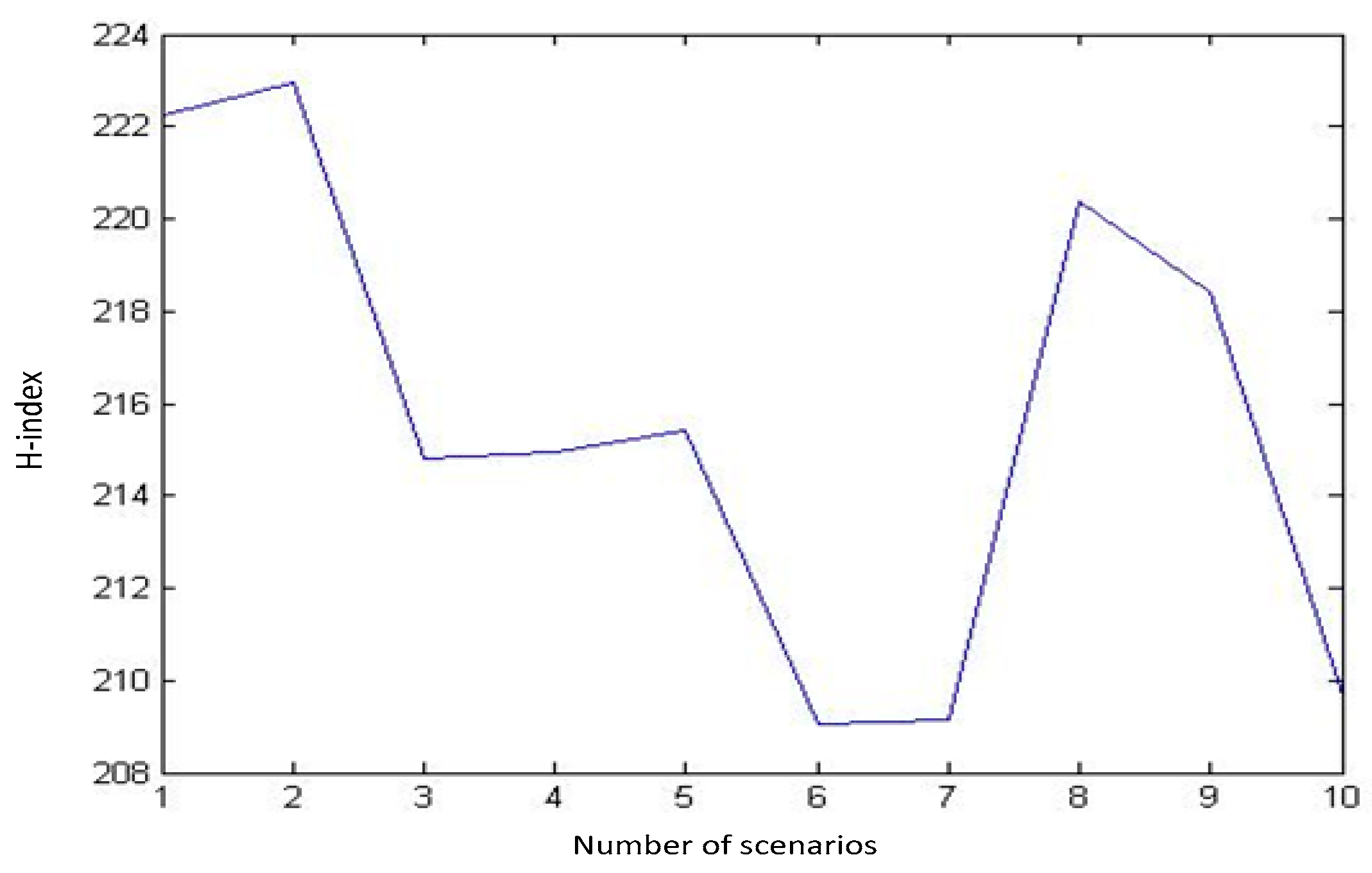
Figure 3.
One hundred randomly generated scenarios and their related H-indexes.

Figure 4.
One thousand randomly generated scenarios and their related H-indexes.
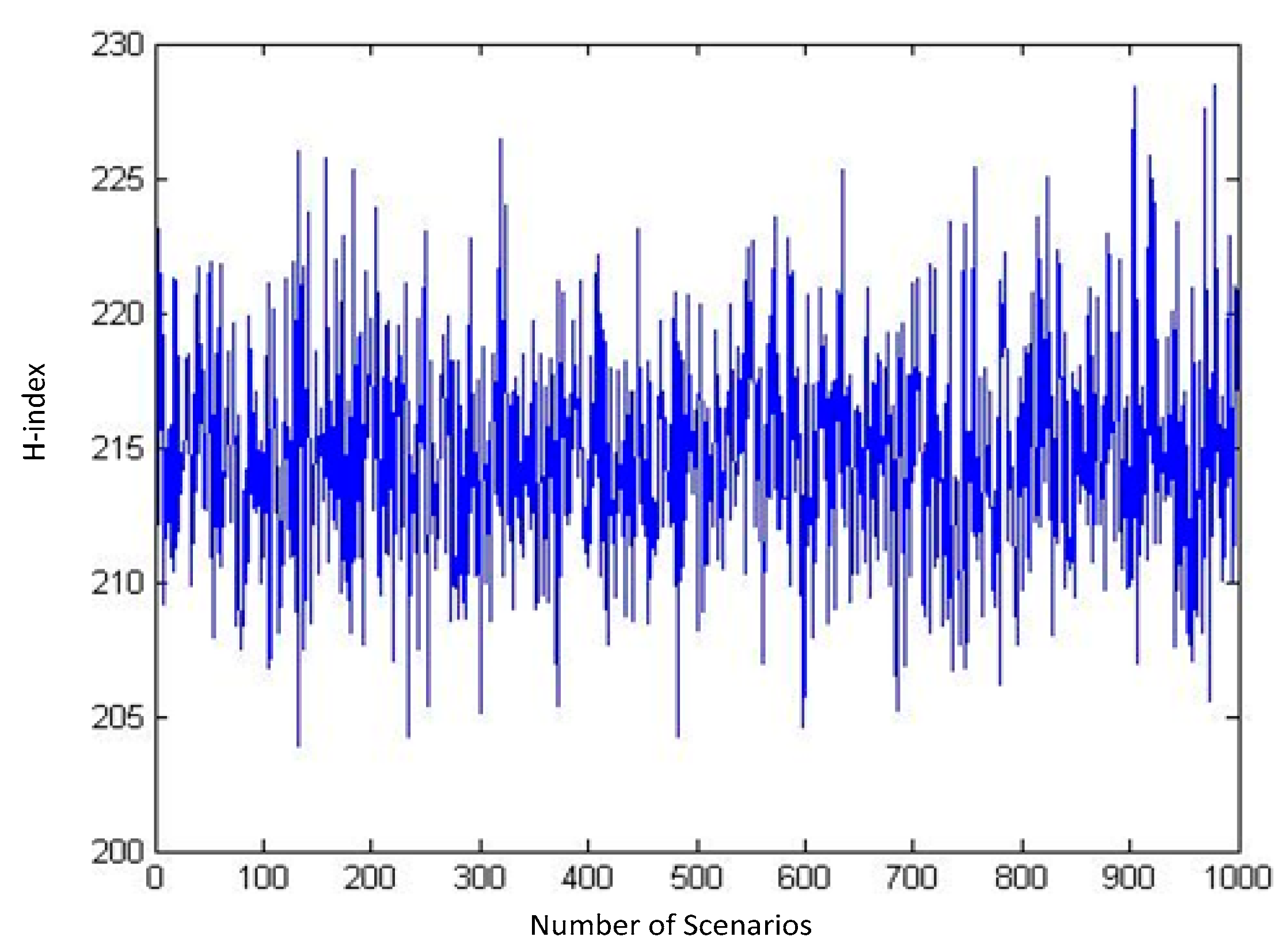
Figure 5.
Three thousand randomly generated scenarios and their related H-indexes.

Figure 6.
Minitab results for scenario generations.
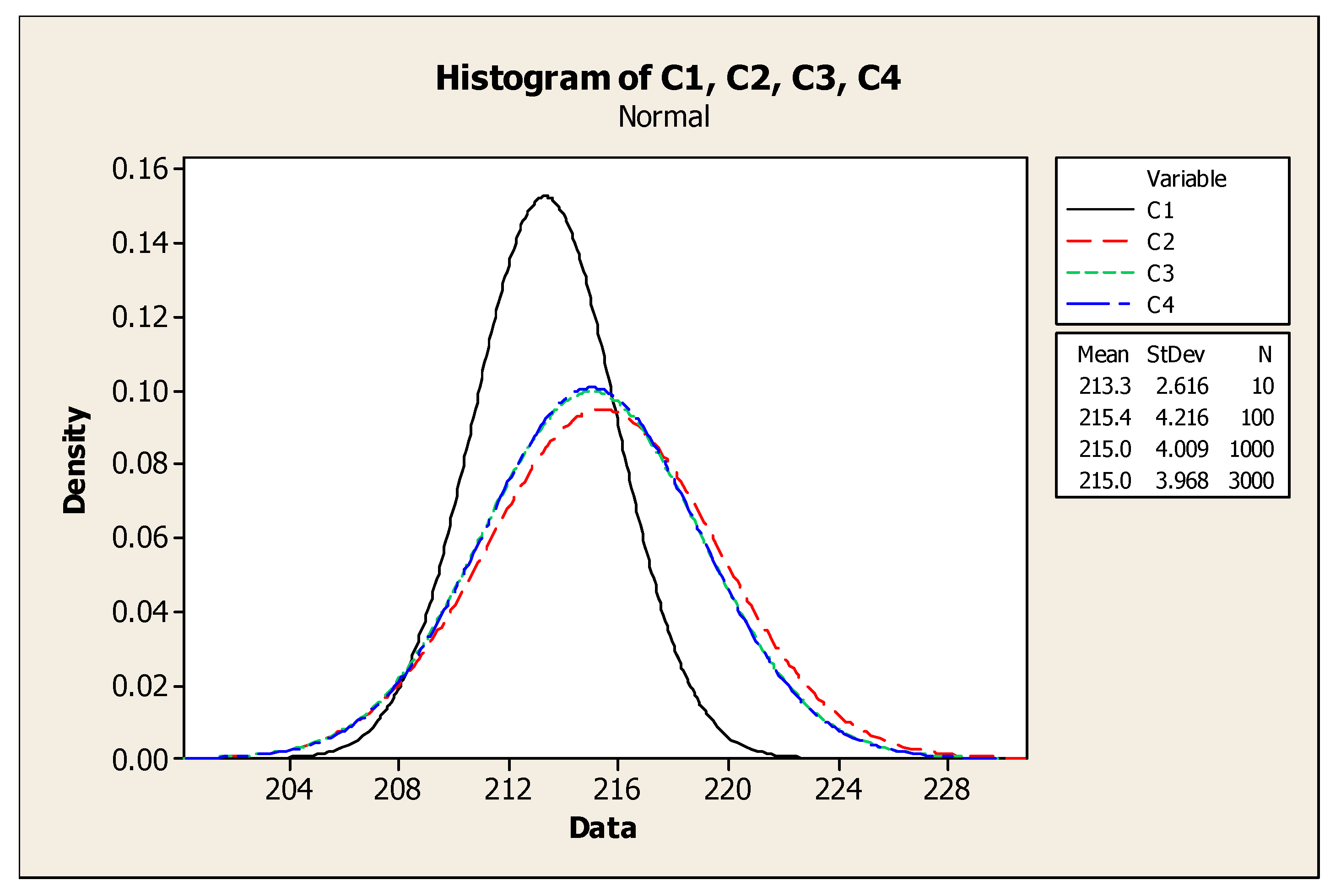
Figure 7.
The outer approximation algorithm.
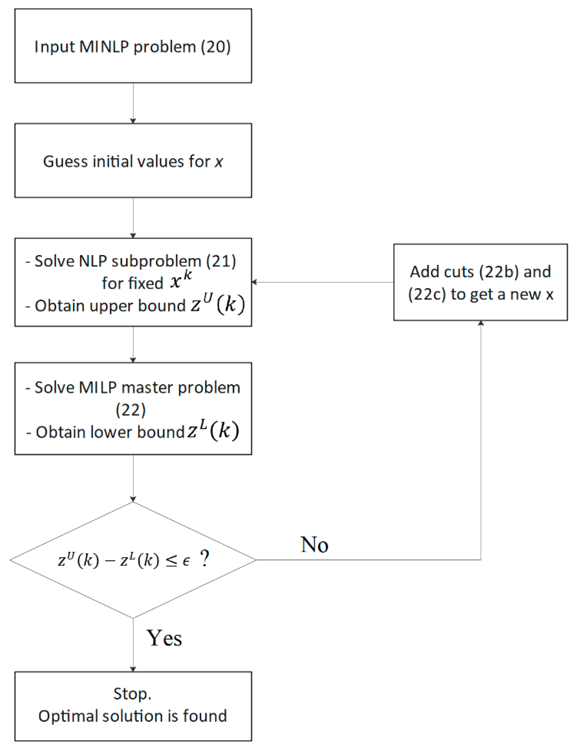
Table 1.
Notations.
| Sets | |
| i | Index of vehicles, i = 1,…, |
| s | Index of scenarios, s = 1,…, |
| Parameters | |
| Demand for bus i at stop k in scenario s | |
| Dwell time of buses at stops, which is constant for all buses at all stops | |
| Passenger arrival rate at stop k in scenario s | |
| Passenger alighting fraction at stop k in scenario s | |
| Running time of bus i from stop k − 1 to stop k in scenario s | |
| Probability of scenario s | |
| Passenger capacity of bus | |
| Sufficiently large number | |
| Variables | |
| Departure time of bus i from stop k in scenario s | |
| Arrival time of bus i at stop k in scenario s | |
| Passengers left behind by full-capacity bus i at stop k in scenario s | |
| The number of passengers in bus i alighting at stop k in scenario s | |
| The number of passengers willing to board bus i at stop k in scenario s | |
| Load in bus i departing stop k in scenario s | |
| 1, if bus i is loaded to capacity when it departs stop k in scenario s 0, otherwise |
Table 2.
Historical data.
| Stops | Passenger Alighting Fraction | Passenger Arrival Rate | Running Time between Stops Plus Acceleration and Deceleration (Minute) |
|---|---|---|---|
| 1 | 1 | 4 | 3 |
| 2 | 0.1 | 1.5 | 3 |
| 3 | 0.1 | 1.5 | 4 |
| 4 | 0.2 | 1.5 | 3 |
| 5 | 0.2 | 2 | 3 |
| 6 | 0.2 | 1.5 | 3 |
| 7 | 0.3 | 2 | 2 |
| 8 | 0.4 | 1.5 | 3 |
| 9 | 0.2 | 2.5 | 3 |
| 10 | 0.1 | 2 | 2 |
| 11 | 1 | 4 | 3 |
| 12 | 0.1 | 2 | 3 |
| 13 | 0.2 | 1.5 | 2 |
| 14 | 0.15 | 1.5 | 3 |
| 15 | 0.3 | 2.5 | 3 |
| 16 | 0.1 | 1.5 | 3 |
| 17 | 0.1 | 2 | 3 |
| 18 | 0.15 | 2 | 3 |
| 19 | 0.2 | 2 | 2 |
| 20 | 0.1 | 2 | 3 |
Table 3.
Departure times of buses from stop 1 in each scenario.
| Buses | Scenario 1 | Scenario 2 | Scenario 3 | Scenario 4 |
|---|---|---|---|---|
| 1 | 354 | 194 | 201 | 256 |
| 2 | 350 | 190 | 197 | 251 |
| 3 | 344 | 187 | 195 | 249 |
| 4 | 339 | 185 | 190 | 244 |
| 5 | 335 | 182 | 189 | 240 |
| 6 | 328 | 179 | 185 | 236 |
| 7 | 325 | 177 | 183 | 233 |
| 8 | 319 | 174 | 180 | 228 |
| 9 | 314 | 170 | 176 | 225 |
| 10 | 308 | 167 | 173 | 220 |
| 11 | 306 | 164 | 170 | 217 |
| 12 | 299 | 160 | 168 | 212 |
| 13 | 294 | 158 | 164 | 208 |
| 14 | 289 | 155 | 160 | 204 |
| 15 | 285 | 151 | 156 | 199 |
Table 4.
Values of objective function due to RP, WS, and EVPI.
| RP | WS | EVPI | |
|---|---|---|---|
| Objective Function | 3.4554 × 10⁸ | 3.4554 × 10⁸ | 0 |
Table 5.
Comparison of computational performance of the OA algorithm and BARON solver.
| OA Algorithm | BARON Solver | |||||||
|---|---|---|---|---|---|---|---|---|
| Solve Time (s) | Solve Time (s) | |||||||
| Test Number | B | S | Avg. | Max | Ratio | Avg. | Max | Ratio |
| 1 | 10 | 20 | 0.92 | 2.34 | 100% | 0.85 | 1.65 | 100% |
| 2 | 15 | 20 | 1.21 | 4.78 | 100% | 0.97 | 2.91 | 100% |
| 3 | 20 | 20 | 5.02 | 7.21 | 100% | 4.63 | 6.77 | 100% |
| 4 | 10 | 25 | 4.67 | 7.40 | 100% | 6.21 | 9.94 | 100% |
| 5 | 15 | 25 | 16.23 | 31.23 | 100% | 462.55 | 924.12 | 100% |
| 6 | 20 | 25 | 52.64 | 65.93 | 100% | 1492.45 | 1800.00 | 80% |
| 7 | 20 | 30 | 183.92 | 229.71 | 100% | 1623.91 | 1800.00 | 20% |
| 8 | 30 | 30 | 514.24 | 852.12 | 100% | 1800.00 | 1800.00 | 0% |
| 9 | 40 | 30 | 1485.76 | 1800.00 | 80% | 1800.00 | 1800.00 | 0% |
| 10 | 50 | 40 | 1800.00 | 1800.00 | 0% | 1800.00 | 1800.00 | 0% |
Publisher’s Note: MDPI stays neutral with regard to jurisdictional claims in published maps and institutional affiliations. |
© 2022 by the authors. Licensee MDPI, Basel, Switzerland. This article is an open access article distributed under the terms and conditions of the Creative Commons Attribution (CC BY) license (https://creativecommons.org/licenses/by/4.0/).
Share and Cite
MDPI and ACS Style
Filabadi, M.D.; Asadi, A.; Giahi, R.; Ardakani, A.T.; Azadeh, A. A New Stochastic Model for Bus Rapid Transit Scheduling with Uncertainty. Future Transp. 2022, 2, 165-183. https://doi.org/10.3390/futuretransp2010009
AMA Style
Filabadi MD, Asadi A, Giahi R, Ardakani AT, Azadeh A. A New Stochastic Model for Bus Rapid Transit Scheduling with Uncertainty. Future Transportation. 2022; 2(1):165-183. https://doi.org/10.3390/futuretransp2010009
Chicago/Turabian StyleFilabadi, Milad Dehghani, Afshin Asadi, Ramin Giahi, Ali Tahanpour Ardakani, and Ali Azadeh. 2022. "A New Stochastic Model for Bus Rapid Transit Scheduling with Uncertainty" Future Transportation 2, no. 1: 165-183. https://doi.org/10.3390/futuretransp2010009