Article

Non-Anatomical Identification and Compositional Profiling of Processed Wood Using ATR-FTIR and Chemometric Modeling

1
Department of Chemistry and Biotechnology, Tallinn University of Technology, Akadeemia tee 15, 12618 Tallinn, Estonia
2
Department of Materials and Environmental Technology, Tallinn University of Technology, Ehitajate tee 5, 19086 Tallinn, Estonia
*
Author to whom correspondence should be addressed.
Analytica 2025, 6(4), 46; https://doi.org/10.3390/analytica6040046
Submission received: 30 September 2025 / Revised: 31 October 2025 / Accepted: 7 November 2025 / Published: 12 November 2025
(This article belongs to the Section Chemometrics)

Abstract

In modern circular-economy value chains, wood is frequently processed into fines, chips, or powders—forms in which anatomical features are no longer visible, rendering traditional visual identification methods ineffective. This study introduces a rapid, non-destructive attenuated total reflection–Fourier transform infrared (ATR-FTIR) spectroscopy approach, combined with chemometric modeling, to address this challenge by enabling both the classification and compositional profiling of processed wood fractions. Using full-spectrum ATR-FTIR data, partial least squares discriminant analysis (PLS-DA) models achieved high-accuracy classification of wood by type, species, and provenance, with sensitivity and specificity reaching up to 1.00. In addition, PLS and backward interval BiPLS models predicted total lignin, acid-soluble lignin, and extractives with strong performance (R2 > 0.90, RPD > 2). Interval selection further enhanced prediction accuracy by reducing RMSEP by up to 30%, improving model stability for real-world application. By replacing slow, reagent-intensive wet chemistry with a rapid, green, and scalable technique, the presented methodology provides a valuable tool for authentication, quality control, and resource optimization when dealing with mechanically processed or recycled wood.

1. Introduction

One of the foremost challenges of the 21st century is the replacement of fossil resources with more sustainable alternatives. One promising alternative is wood. Wood is a highly abundant, renewable, and universal feedstock with many useful applications, such as paper pulp production, building and furniture, natural reinforcement in polymer composites, and the production of biofuels, advanced materials, and chemicals [1]. Wood is the main natural resource in Estonia—Estonian forest land has an area of 2.3 million hectares (data for the year 2023), making up more than half of Estonia’s total land area [2]. The utmost importance of the forests and the need for their versatile use promote the transition of the forest sector to a circular bioeconomy, which is one of the most critical goals in this area.
Over the years, a variety of new lignocellulosic-biomass-processing technologies and strategies have been developed. Cellulose and hemicellulose are depolymerized into sugars, which can then be converted into bioethanol or biobutanol through various biological pathways or chemical processing. Lignin (up to 25–30% of the wood mass) is a highly branched, cross-linked, amorphous polymer consisting mainly of phenylpropane monomers (monolignols) joined by C-C and C-O-C chemical bonds. It can be depolymerized to produce aromatics or valorized to other value-added products, such as different thermoplastic or lignin-based biocomposite materials [3].
The type and composition of wood species determine their suitability for pulping and other biorefinery strategies and processing technologies. Microscopically, wood species can be identified by visual appearance, like the color of sapwood and hardwood, the width of their annual rings, the hardness of their surface, the gloss of their wooden surface, and anatomical features like rays, vessels, tracheids, etc. [4]. However, the visual examination of wood chips or milled wood residues does not facilitate the identification of an unknown wood sample, as it does not reveal the chemical composition of the wood. Therefore, the identification of wood chips or wood residues requires analytical techniques that provide for the qualitative as well as quantitative determination of their chemical composition.
Wet chemistry methods are currently the preferred approach to yield accurate and precise results. However, the chemical characterization of wood samples is a complex procedure involving several steps wherein wood biomass is extracted with organic solvents to remove extractives (terpenes, fats, waxes, and phenolics), followed by the isolation of wood components or their degradation to monomeric fragments (Van Soest and Klason methods). These traditional wet laboratory methods are tedious and time-consuming, require large sample sizes, and involve hazardous chemicals.
The advantage of using vibrational spectroscopic techniques, such as attenuated total reflectance–Fourier transform mid-infrared spectroscopy (ATR-FTIR) [5,6], stems from the possibility of evaluating the composition of lignocellulosics by analyzing a small number of samples and developing non-destructive, simple, fast, and direct determination methods. The use of this technique coincides with trends in wood analysis to develop green methods that generate fast responses with no consumption of reagents or solvents, consequently producing less of an environmental impact.
Exploratory and quantitative methods employing vibration spectroscopic techniques require the joint use of chemometric tools. Among spectroscopic methods, near-infrared spectroscopy (NIR) in combination with chemometric methods is being intensively applied for the classification and quantitative characterization of pulp, wood, and non-wood biomass [7,8,9,10,11,12,13,14].
So far, FTIR spectroscopy has been mostly applied to the qualitative identification and differentiation of woody matrices by using multivariate statistical analysis, including principal component analysis (PCA), hierarchical cluster analysis (HCA), and linear discrimination analysis (LDA) [5,15,16,17]. Critically, though, the application of ATR-FTIR spectroscopy for the quantitative prediction of lignocellulose contents in wood samples is limited [18]. In comparison with FT-NIR spectroscopy, ATR-FTIR spectroscopy tends to have lower prediction accuracy and robustness [19,20]. However, the performance of partial least squares regression (PLSR) models for the quantitative prediction of wood components could be improved through the application of interval variable selection algorithms to the spectral data [6]. Variable selection methods are useful for deleting irrelevant and noisy variables, improving the performance and robustness of the method, increasing the signal-to-noise ratio, and reducing the model complexity [21]. The interval partial least squares (iPLS) method [22] is the most common continuous variable selection method based on the continuous screening of informative vectors estimated from multivariate models.
The objective of this study is to establish a non-destructive, scalable approach for identifying and characterizing mechanically processed wood, where conventional anatomical methods no longer apply. We employ ATR-FTIR spectroscopy coupled with chemometric modeling to (i) classify material by type (hardwood vs. softwood), species, and provenance using full-spectrum information, and (ii) predict key chemical attributes—total lignin, acid-soluble lignin, and extractives—using PLS-based calibrations. We further examine spectral interval selection to enhance predictive accuracy and model robustness. Overall, the approach is positioned as a rapid, green alternative to wet chemistry for quality control, authentication, and resource optimization within circular bioeconomy value chains, especially when anatomy is absent in processed or recycled wood.

2. Materials and Methods

2.1. Samples

A total of ninety-two wood samples (10–15 cm in diameter) from silver birch (Betula pendula Roth), Norway spruce (Picea abies), and Scots pine (Pinus sylvestris) were collected from two major forest regions in Estonia (Table 1). Forests managed by the Estonian State Forestry Company were selected for sample collection based on distinct growing site types: stands in Võrumaa county in southern Estonia (characterized by dry sandy soils) and Raplamaa county in northern Estonia (characterized by wet loam and limestone soils).
Forty-seven samples were collected from the stumps of freshly felled logs at three different logging sites in Võrumaa county, with distances of approximately 10–30 km between the sites. From each site, an average of five birch, five spruce, and five pine samples (10–15 cm in diameter) were collected. Forty-five additional samples were similarly collected from stumps of freshly felled logs at three logging sites in Raplamaa county, also spaced approximately 10–30 km apart.
After collection, the bark was removed from the wood samples by mechanically cutting it off. A panel saw with a circular blade designed for ripping was used to produce large wood shavings along the grain. The shavings were then air-dried and milled using a Fritsch Pulverisette 29 mini mill equipped with a 0.25 mm trapezoidal perforation sieve insert. The remaining moisture contents were measured before analysis. Prior to ATR-FTIR acquisition, the samples were dried at 105 °C overnight to eliminate any residual moisture.

2.2. Characterization of Wood Samples by Chemical Methods

For the measurement of the metal contents (Na, K, Cu, Zn, Pb, Cd, and Ni) milled wood samples were microwave-digested in a mixture of strong acids in accordance with ISO 3884 standard procedure [23], diluted, and subjected to analysis by flame and electrothermal atomic absorption spectrometry (AAS). Atomic absorbance spectrometer with graphite furnace (SpectrAA 220Z, Varian Instruments, Palo Alto, CA, USA) was used for determination of Pb, Cu, Cd, and Ni. Flame atomic absorbance spectrometer (AASF) (SpectrAA 220F, Varian Instruments, Palo Alto, CA, USA) was used for determination of Na, K, and Zn.
Organic elements CHNO were measured by the standard test method ISO 21663 [24]. For that, an Elementar vario MICRO cube was used. Samples were oxidized in the combustion tube at 1150 °C in the presence of oxygen, using tungsten(VI)-oxide granulate as a catalyst. The resulting gaseous reaction products were separated in an adsorption column and subsequently measured using a thermal conductivity detector. Helium served as the carrier gas. For oxygen determination a pyrolysis column packed with carbon was used.
Extractive content (EA) was determined in accordance with ASTM D1107-96 [25]. Approximately 2.0 g of milled wood was placed in a Soxhlet thimble and extracted under reflux with an ethanol–toluene mixture (200 mL: 85 mL, v/v) for 6 h. The extract was allowed to cool, the solvent was evaporated, and the residue was dried to constant mass. The mass of the dried residue was taken as the extractive content.
Klason (acid-insoluble) lignin was determined by two-stage sulfuric acid hydrolysis of the carbohydrate matrix (ASTM D1106-96) [26]. Approximately 0.5 g of milled biomass was first treated with 72 wt% H2SO4 at 20–25 °C (≈1 h) with intermittent stirring, then diluted to ~3 wt% H2SO4 and hydrolyzed at 121 °C for 60 min in an autoclave. The hydrolysate was vacuum-filtered through a tared, medium-porosity crucible; the washed and dried acid-insoluble residue was taken as acid-insoluble lignin (AIL). Acid-soluble lignin (ASL) was quantified separately from the filtrate by UV absorbance and added to obtain total lignin (TL) in accordance with NREL/TP-510-42618 [27].

2.3. Collection and Pre-Processing of Spectral Data

ATR-FTIR spectra of wood samples were recorded on a IRTracer-100 (Shimadzu Scientific Instruments, Tokyo, Japan) instrument equipped with a diamond ATR (Specac) and a DLaTGS detector. Thin wood sections were measured under constant contact pressure using the accessory’s pressure knob. Spectra were acquired over 4000–400 cm−1 at 4 cm−1 spectral resolution with 32 co-added scans. Data were exported on a zero-filled grid with a 0.96 cm−1 point spacing (data interval). After edge trimming, the working matrix comprised 3734 variables. The 32-scan averages for each sample were used for subsequent chemometric analysis. To remove an unimportant baseline signal from the samples by taking the derivative of the measured responses with respect to the wavenumbers, the Savitzky–Golay derivatization algorithm [28] was applied first to the spectral data (size of the window 15, the second order of the polynomial, and the first order of the derivative). Then, processed spectra were normalized using a standard normal variate (SNV) transformation (weighted normalization) and autoscaled. Spectrum processing, PLS model construction, and variable selection methods were applied to the data using the Solo software 9.2(Eigenvector Research Inc., Manson, WA, USA).

2.4. Multivariate Analysis Methods (Data Analysis, Discrimination, and Model Development)

In the present study, PCA was utilized as an unsupervised multivariate data analysis tool, whereas a partial least squares discriminant analysis (PLS-DA) and PLSR were both employed as supervised multivariate analysis tools for the discrimination of wood samples and quantitative prediction of their biocomposition, respectively.
PCA is a multivariate statistical technique used to extract and interpret the systematic variance in a dataset. Generally, PCA modeling replaces a complex multi-dimensional dataset with a simplified one. When data are converted into the dimensionally reduced PCA space, the input dataset is decomposed into two matrices: scores and loadings [29]. The PCA was performed on the chemical and spectral data of all 92 samples by using a singular value decomposition (SVD) algorithm and a 10-fold Venetian blind cross-validation procedure to enhance model optimization. Q residuals and Hotelling’s T2 statistic were used to examine any possible grouping and to identify potential outliers by studying score plots [30].
PLS-DA is a chemometric tool that utilizes a PLS algorithm in modeling differences between defined sample classes, thereby allowing for the discrimination of samples within these groups [31]. PLS-DA models were built for the discrimination of wood species, wood type, and place of growth (Table 2). The dataset was divided into a calibration set (CS) and a prediction set (PS) using the Kennard–Stone (KS) method [32], with two-thirds of the dataset allocated to the CS and one-third of the dataset to the PS. The KS method selects a subset of samples that uniformly covers the dataset and includes exterior samples as the calibration set by maximizing the Euclidean distances between the remaining and selected objects. The remainder are placed in the test set. As a result, the CS for this study consisted of 61 samples, while the PS comprised 31 samples. In building the supervised PLS-DA models, a certain class/es was/were assigned to wood samples, and the optimum PLS-DA model was determined by the minimum root mean square error of cross-validation (RMSECV) of the calibration set. A 10-fold Venetian blind cross-validation was used in building the PLS-DA models. The cross-validation technique rotates the membership of the samples during calibration to ensure that the results (i.e., the CS and PS) are not membership-dependent and to ensure that the model is not overfitting the data [33]. The PLS-DA model performance was evaluated based on the metrics of accuracy: sensitivity, specificity, class error (the average false positive rate and false negative rate for a class (Class Err. = 1 − (sensitivity + specificity)/2)), and the root mean square error of estimation (RMSEE), cross-validation (RMSECV), and prediction (RMSEP).
The full-spectrum (4000–400 cm−1) PLSR and backward interval PLS (BiPLS) models were developed to predict total lignin, acid-soluble lignin, and extractive content in wood. PLS projects the predictor variables and the observed variables into a new space and then captures several latent variables (LVs) that can represent the majority of raw information, using them to establish a linear regression model. The LVs that explained the most variance in the data were used to build regression models. For PLS modeling, the cross-validation and calibration/prediction sample selection strategies were similar to the PLS-DA ones. The optimal number of LVs was selected according to the RMSECV value during the 10-fold Venetian blind cross-validation of the calibration models. The number of factors where the first minimum value of RMSECV appeared was the optimal number of LVs.
To improve the performance and robustness of the PLS models, a BiPLS was applied [22]. The BiPLS model is an effective characteristic variable selection algorithm proposed on the basis of interval partial least squares (iPLS) [34,35]. This model divides the dataset into a given number of intervals of equal length and calculates RMSECV with each interval left out, leaving out one interval at a time. After this process, the most relevant intervals are left behind, and spectral regions containing noise or irrelevant information are discarded.
Predictions were carried out using the samples from the PS. The performance and reliability of the predictive PLS models were assessed based on several evaluation metrics, including coefficients of multiple determination for calibration (R2cal) and prediction (R2pred), which indicate the proportion of variance in the predicted variable that can be explained by the model; RMSEC, RMSEP, and residual predictive deviation (RPD). Good models have a low root mean square error (RMSE), a high coefficient of multiple determination (R2) (close to 1) and RPD (>2), and an RMSEP lower than the RMSECV.

3. Results

3.1. Characterization of Wood Samples

Table 2 presents the measured values (average and range) for seven biometal and heavy metals contents (Zn, Na, K, Cu, Pb, Cd, and Ni), elemental contents (CHNO), total lignin (TL), acid-soluble lignin (ASL), and extractive (EA) content in soft and hard woods grown in different regions of Estonia. Trace metals play a significant role in the processing behavior, environmental impact, and downstream applications of wood-based materials. Metals, which originate from the wood itself and vary depending on species and site-specific soil conditions, can significantly affect the efficiency of biorefinery processes (e.g., pulping, hydrolysis, and combustion) and the quality of final products. The amplitudes of the values estimated for metals in birch, pine, and spruce were within the ranges obtained in previous studies of Estonian [36,37] and European wood [38,39]. The results for the elemental contents in wood were also consistent with the available data for the CHNO composition of wood, though the sulfur content was below the limit of quantitation (0.01 mg/kg) for all wood samples.
The total lignin content was obtained as the sum of the lignin amount obtained with the Klason method and the acid-soluble lignin, measured spectrophotometrically. Acid-soluble lignin is composed of low-molecular-weight degradation products and hydrophilic derivatives of lignin, and its formation is dependent on the type of wood—the almost five times higher acid-soluble lignin content obtained for birch samples compared to other types of wood confirmed that the syringyl lignin was dissolved in 72% sulfuric acid more rapidly [40].
Extractives, mainly consisting of fats, fatty acids, waxes, sterols, tannins, and polyphenols, represent a minor component, often constituting less than 10% of wood [41]. However, they contribute significantly to the characteristics of wood and its usage. Notably, the amount of extractives in wood varies greatly [42]. In our results, the highest average extractive content was found in pine samples (around 6% per dry matter).

3.2. Principal Component Analysis on Chemical Data

With the aid of multivariate analysis, it is possible to condense information contained in data with a reduced number of dimensions, as well as to evaluate possible differences or similarities between observations and variables. A PCA was carried out on scaled and normalized chemical data obtained for 92 wood samples (averaged data is presented in Table 1). Three different classes (and sub-classes) were assigned to the wood samples before the PCA (Table 1). The data came from metal analysis, while the organic elemental content and biocomposition (extractives, total lignin, and acid-soluble lignin) of the wood were analyzed separately (Figure 1a–f). The score scatter plots of the first two principal components (PCs) for the wood samples analyzed for metals, CHNO contents, and biocomposition accounted for 51.2%, 61.8%, and 92.5% of the total variability, respectively. Despite the comparably low percentage of explained variance for the first two PCs for metal and elemental content data, the samples were clearly grouped into two clusters based on their distribution along PC 1 (Figure 1a–c): one group with negative PC 1 scores (softwoods) and another group with scores located on the positive side of PC 1 (hardwoods). Moreover, the PCA of the elemental content data separated the samples along PC 2 according to the place of growth: northern and southern Estonia (Figure 1d). A similar grouping of the hardwoods and softwoods was obtained for biocomposition data (Figure 1e,f), where some differentiation between the softwood species pine and spruce could additionally be observed (Figure 1e).
The loading plots in coordinates PC 1 vs. PC 2 gave vectors on the score plots (Figure 1a–f). These vectors provided information on chemical parameter(s), which in turn contributed to the separation of wood samples according to their PC 1/PC 2 values. Samples tended to cluster according to the variability of either their contents of heavy metals Pb, Zn, and Cd (Figure 1a,b) or of organic elements—hardwood grown in Estonia has a higher nitrogen and oxygen content compared to softwood (Figure 1c). The place of growth of the wood defined the differentiation of the samples along PC2 due to higher C and O contents in woods grown in the south (Figure 1d). The loading plot of biocomposition (Figure 1e,f) indicated that pine has a higher extractive content than spruce, which led to the samples being spread in a horizontal direction, and a lower lignin content in birch caused the samples to separate along PC1 in a vertical direction. Indeed, hardwood samples contain less lignin than their softwood counterparts [43].

3.3. Characteristic Bands in the FTIR Absorption Spectra of Wood Samples

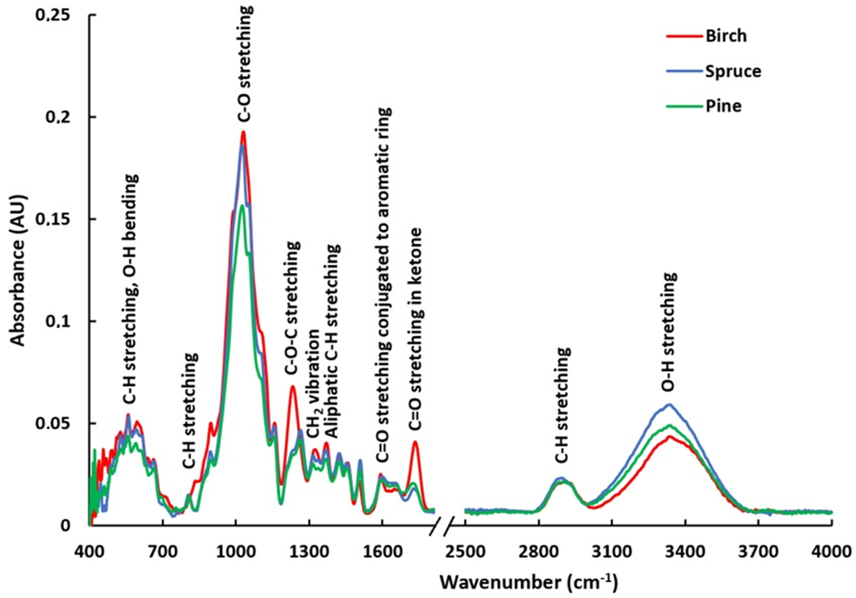
Figure 2 displays the raw spectra of the representative samples of birch, spruce, and pine. Detailed peak positions and wood sample assignments are listed in Table 3. Owing to the chemical complexity of wood, the fingerprint region contains numerous characteristic bands, and assigning every peak to a specific constituent is challenging. In this study, we assigned as many peaks as possible to wood components using available published data. The spectra of all the wood samples presented a broad and intense band in the region from 3600 to 3000 cm−1 related to the O-H absorption of water and O-H stretching caused by inter- as well as intra-molecular hydrogen bonding in the cellulose component of the wood. The peak at 2927 cm−1 revealed the presence of CH stretching vibrations of the cellulose molecule. In the fingerprint region, the spectra were very complex, containing many bands assigned to the main wood components. The band at 1740–1730 cm−1 was assigned to the characteristic C=O stretching vibrations in unconjugated ketone, carbonyl, and aliphatic groups of xylan commonly found in hemicellulose and lignin. The bands at 1592, 1508–1503, 1323, and 1232 cm−1 were assigned to the characteristic bending or stretching of different groups of lignin. The main characteristic peaks, which were the stretching vibrations of C=O, aromatics, and C–O, were around 1640, 1510, and 1030 cm−1. However, in the different types of wood, the positions and relative intensity of the peaks differed.
Softwoods and hardwoods differ in chemical composition, including their lignin units (guaiacyl vs. syringyl–guaiacyl), hemicelluloses (e.g., xylans, glucomannans, mannan-derived constituents), and profiles of low-molecular-weight extractives. The band intensity at 1733 cm−1 was greater in the hardwood (birch) than in the softwoods (pine and spruce). Furthermore, the peak around 1232 cm−1 caused by syringyl lignin seemed significantly more intense in the spectra of birch compared to spruce and pine FTIR spectra, and the peak at 1270 cm−1 caused by guaiacyl lignin is present only in the softwood sample [44]. Moreover, small shifts in the band maxima around 1505 and 1730 cm−1 for softwoods (1508 and 1725 cm−1) and hardwoods (1503 and 1735 cm−1), coming from different wood characteristics (S/G lignin ratio, hemicellulose types/acetylation) and the local bonding environment (H-bonding, conjugation, matrix effects), also make chemical sense. These spectral differences, in combination with multivariate chemometric approaches, can be used to better discriminate between softwood and hardwood and to establish calibration models for the quantitative analysis of the biocomposition of woods.

3.4. Principal Component Analysis on Spectral Data

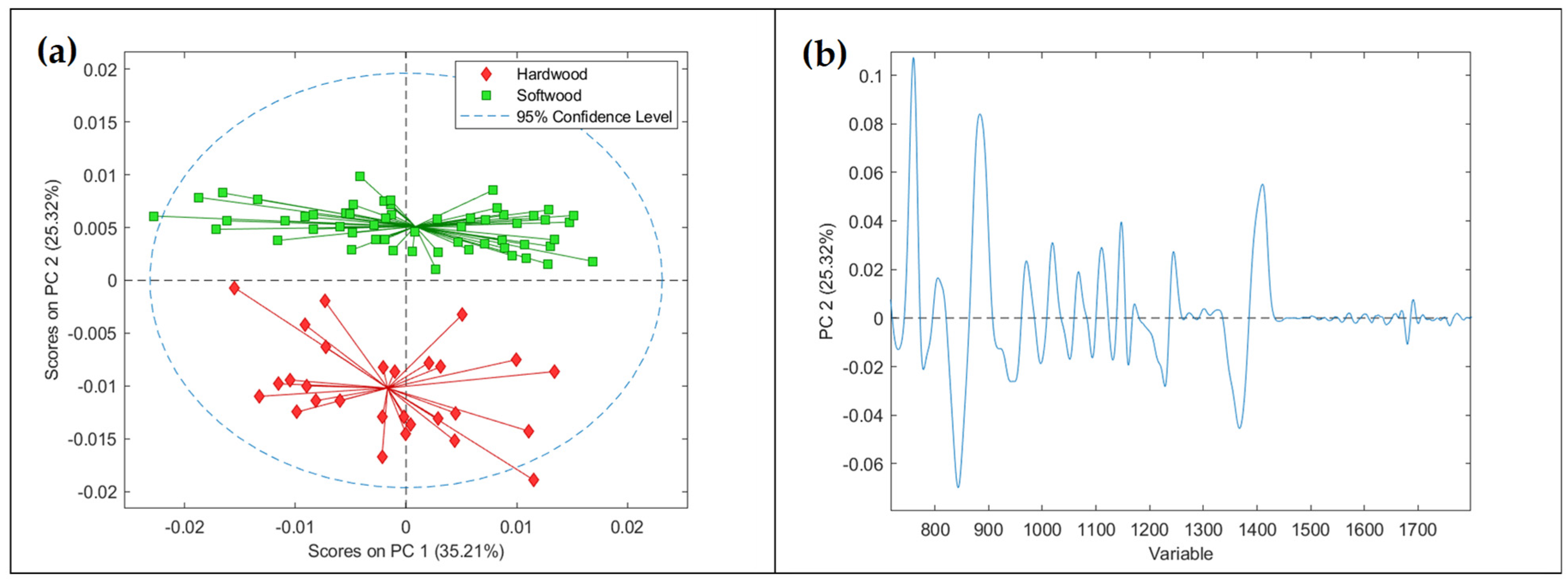
The PCA was performed for pre-processed spectral data, and the first, second, and third PCs accounted for 35.2%, 25.3%, and 8.4% of variability, respectively. The score plots clearly indicated that hardwood and softwood samples were well differentiated among themselves: hardwoods had negative PC 2 scores, while softwood scores were located on the positive side of PC 2 (Figure 3a).
Softwood and hardwood differ in their chemical composition due to the different ratios of various monolignols, guaiacyl (G), or syringyl (S) propane units in lignin, hemicelluloses, and wood extractives [41,43]. The amount of lignin is also higher in softwood as compared to hardwood.
The relationship between PC2 and the chemical constituents of wood samples associated with it was established by developing a loading plot using PC2 vs. the variable (wave)number (Figure 3b). This sub-spectrum showed which wavenumbers mostly contributed to the grouping of wood samples along the PC2 direction. According to this plot, intensive negative and positive bands at 1457, 1370, 1232, 1323, and 895 cm−1 indicated the presence of characteristic C-H stretching in the methyl group or the aromatic ring and guaiacyl and syringyl units in lignin, which are mainly responsible for the differentiation of softwood and hardwood samples.

3.5. PLS-DA Modeling Results

The PLS-DA models were built to discriminate between wood species, wood types, and places of growth. The optimum PLS-DA model was determined using the RMSECV of the training set. This procedure resulted in the selection of three LVs for the models based on spectral data and three or four LVs for models built on chemical data. Table 4 shows a summary of the performance of the best selected PLS-DA models.
The captured variability of the obtained PLS-DA models discriminating hardwood from softwood was around 65% within the FTIR spectra dataset and varied from 77 to 100% for chemical data (CHNO, metals, biocomposition). Hardwood/softwood discrimination models yielded a class error close to zero during training and 0–0.06 for prediction within all the data. Validation of the models on the test set yielded the maximum sensitivity and specificity (1.0) for spectral data and close to 1.0 for chemical data. A plot of the class predictions is shown in Figure 4. In the model built on elemental content, three latent variables were adopted, and they accounted for 77% of the variability in the dataset. This approach also provided very good discriminating ability for woods centered on the place of growth. Woods grown in northern Estonia were differentiated from the woods grown in southern Estonia with a sensitivity and specificity of 0.98 and 0.97, respectively, for training, and 0.9 and 1.0 for the test sets. The PLS-DA models discriminating wood species were built using the first three or four factors, which accounted for 63–100% of the total variance within the dataset (Table 4). The PLS-DA models of wood species provided excellent discrimination of birch: a class error of 0.0 in training and 0.0 in prediction within the FTIR dataset and a class error of 0–0.07 in training and 0.09–0.12 in prediction for models based on metals content and biocomposition datasets. A comparably good discrimination of softwoods (pine and spruce), which have quite a similar chemical composition, was also obtained by applying the PLS-DA to spectral and chemical datasets. The pine and spruce PLS-DA models yielded sensitivities and specificities in the range of 0.80–1.0 and 0.71–0.93, respectively, for the training and 0.50–0.90 and 0.57–0.86 for the test sets.
In the PLS-DA models based on FTIR spectra, peaks at 895, 1232, and 1370 cm−1 were responsible for the discrimination of hardwood and birch from other woods. The peaks at 895 and 1232 cm−1 were consistent with the aromatic ring of lignin (Table 3), whereas the peak at 1370 cm−1 coincided with CH3 bending vibration. In elemental content models, regression vectors showed major contributions from nitrogen and oxygen content in the discrimination between hardwood and softwood, while hydrogen content contributed to the differentiation of wood depending on the place of growth. The regression vectors of the metals PLS-DA model showed that the concentrations of Zn, Na, and Pb were the most relevant for the discrimination of hardwoods and birch, while the regression vectors of the biocomposition PLS-DA model indicated that the concentration of acid-soluble lignin was the most relevant.

3.6. PLS Modeling Results

A PLS model was applied to the experimental dataset in order to predict total lignin, acid-soluble lignin, and extractive contents in wood samples. The appropriate number of LVs included in the PLS models ranged between 5 and 7, depending on the parameter studied. This number was selected according to the minimum value of the RMSECV during the 10-fold Venetian blind cross-validation of the calibration models.
The developed full-spectrum PLS models demonstrated satisfactory performance in predicting the wood characteristics, with coefficients of multiple determination for calibration (R2cal) above 0.9 and residual predictive deviation (RPD) above 2 (Table 4). However, models based on the full FTIR spectra still showed low stability, as their RMSECV and RMSEP values were quite different [45]. This could be attributed to the fact that the ATR-FTIR spectra still contained a large amount of information that was not related to a given parameter of interest while building the multivariate calibration models. Thus, the use of variable selection techniques allowed for the selection of spectral regions related to the outcome of interest, producing simpler and more robust models. Consequently, despite the PLS models having presented satisfactory performance, a BiPLS algorithm [35] was also tested.
For the BiPLS method, all intervals are initially included in the models, and the algorithm selects single intervals to discard. In the present study, to select the FTIR characteristic intervals, the interval size varied from 500 to 100 variables, and the number of division intervals was determined automatically. Thus, the BiPLS algorithm was initially applied by splitting the full spectra into seven intervals, increasing the number of intervals to 36. The best RMSECV values were provided by models with the smallest size of intervals (100 variables) and a selected number of variables of 1934 for Klason lignin, 834 for acid-soluble lignin, and 934 for extractives.
In comparison to the full-spectrum models, the BiPLS model decreased RMSEP, the main parameter for evaluating the model quality/trueness, by up to 3% for Klason lignin, up to 10% for acid-soluble lignin, and up to 30% for extractives (Table 5). Furthermore, the optimized models had closer RMSECV and RMSEP values, which reflected their better performance and improved stability in comparison to the full-range PLS model.
Overall, the BiPLS model achieved good results, demonstrating a strong correlation between the analyzed variables, a satisfactory fit to the data, and minimal prediction errors. These findings highlight the effectiveness of using FTIR analysis in conjunction with chemometric methods for predicting the content of wood components.

4. Conclusions

This study demonstrates that ATR-FTIR spectroscopy combined with chemometric modeling provides an effective and non-destructive approach for the classification and compositional analysis of fine wood fractions in which anatomical features are no longer visible due to mechanical processing. Such an approach is particularly valuable for supporting quality control, material traceability, and resource optimization in circular bioeconomy value chains.
Using full-spectrum ATR-FTIR data, PLS-DA models achieved high classification accuracy for hardwood and softwood types, with sensitivity and specificity reaching up to 1.00 under cross-validation and external validation. The models also showed good performance for more complex classification tasks, including species- and provenance-level separation, with classification errors remaining low across independent test sets.

Author Contributions

O.-S.S.: methodology, investigation, formal analysis, visualization, writing—original draft preparation, and writing—review and editing. J.K.: resources, writing—review and editing, and funding acquisition. M.K.: conceptualization, methodology, supervision, writing—original draft preparation, writing—review and editing, and funding acquisition. All authors have read and agreed to the published version of the manuscript.

Funding

This research was funded by the Estonian Research Council via projects RESTA11, TEM-TA49 and TEM-TA139.

Data Availability Statement

The original contributions presented in this study are partially included in the article. The raw data supporting the conclusions of this article will be made available by the authors on request. Further inquiries can be directed to the corresponding author.

Acknowledgments

The authors gratefully acknowledge Alar Konist’s laboratory for performing CHNO analysis of the wood samples.

Conflicts of Interest

The authors declare no conflicts of interest.

Abbreviations

The following abbreviations are used in this manuscript:
PLSPartial Least Squares
ATR-FTIRAttenuated total reflection Fourier-transform infrared spectroscopy
Bi-PLSBackward interval Partial Least Squares
RPDResidual Predictive Deviation
PCAPrincipal Component Analysis
PLS-DAPartial Least Squares Discriminant Analysis
ASLAcid-soluble lignin
TLTotal lignin
EAExtractives

References

  1. Sulis, D.B.; Lavoine, N.; Sederoff, H.; Jiang, X.; Marques, B.M.; Lan, K.; Cofre-Vega, C.; Barrangou, R.; Wang, J.P. Advances in lignocellulosic feedstocks for bioenergy and bioproducts. Nat. Commun. 2025, 16, 1244–1253. [Google Scholar] [CrossRef]
  2. Keskkonnaportaal. Metsamaa, sh Kaitsealuse Metsamaa Osakaal Eestis. Available online: https://keskkonnaportaal.ee/et/metsamaa-sh-kaitsealuse-metsamaa-osakaal-eestis (accessed on 10 September 2025).
  3. Zhou, N.; Thilakarathna, W.P.D.W.; He, Q.S.; Rupasinghe, H.P.V. A Review: Depolymerization of Lignin to Generate High-Value Bio-Products: Opportunities, Challenges, and Prospects. Front. Energy Res. 2022, 9, 2021–2027. [Google Scholar] [CrossRef]
  4. Ruffinatto, F.; Crivellaro, A.; Wiedenhoeft, A.C. Review of Macroscopic Features for Hardwood and Softwood Identification and a Proposal for a New Character List. IAWA J. 2015, 36, 208–241. [Google Scholar] [CrossRef]
  5. Sharma, V.; Yadav, J.; Kumar, R.; Tesarova, D.; Ekielski, A.; Mishra, P.K. On the rapid and non-destructive approach for wood identification using ATR-FTIR spectroscopy and chemometric methods. Vib. Spectrosc. 2020, 110, 103097. [Google Scholar] [CrossRef]
  6. Miaw, C.S.W.; Assis, C.; Silva, A.R.C.S.; Cunha, M.L.; Sena, M.M.; de Souza, S.V.C. Determination of main fruits in adulterated nectars by ATR-FTIR spectroscopy combined with multivariate calibration and variable selection methods. Food Chem. 2018, 254, 272–280. [Google Scholar] [CrossRef] [PubMed]
  7. Liu, J.; Jin, S.; Bao, C.; Sun, Y.; Li, W. Rapid determination of lignocellulose in corn stover based on near-infrared reflectance spectroscopy and chemometrics methods. Bioresour. Technol. 2021, 321, 124449. [Google Scholar] [CrossRef] [PubMed]
  8. Uddin, M.N.; Ferdous, T.; Islam, Z.; Jahan, M.S.; Quaiyyum, M. Development of chemometric model for characterization of non-wood by FT-NIR data. J. Bioresour. Bioprod. 2020, 5, 196–203. [Google Scholar] [CrossRef]
  9. Pastore, T.C.M.; Braga, J.W.B.; Coradin, V.T.R.; Magalhães, W.L.E.; Okino, E.Y.A.; Camargos, J.A.A.; Muñiz, G.I.B.D.; Bressan, O.A.; Davrieux, F. Near infrared spectroscopy (NIRS) as a potential tool for monitoring trade of similar woods: Discrimination of true mahogany, cedar, andiroba, and curupixá. Holzforschung 2011, 65, 73–80. [Google Scholar] [CrossRef]
  10. Xie, H.; Chen, Z.-G. Application of genetic simulated annealing algorithm in detection of corn straw cellulose. Chin. J. Anal. Chem. 2019, 47, 1987–1994. [Google Scholar]
  11. Alves, A.; Santos, A.; da Silva Perez, D.; Rodrigues, J.; Pereira, H.; Simões, R.; Schwanninger, M. NIR PLSR model selection for Kappa number prediction of maritime pine Kraft pulps. Wood Sci. Technol. 2007, 41, 491–499. [Google Scholar] [CrossRef]
  12. Kothiyal, V.; Jaideep; Bhandari, S.; Ginwal, H.S.; Gupta, S. Multi-species NIR calibration for estimating holocellulose in plantation timber. Wood Sci. Technol. 2015, 49, 769–793. [Google Scholar] [CrossRef]
  13. Fišerová, M.; Gigac, J.; Russ, A.; Maholányiová, M. Using niranalysis for determination of hardwood kraft pulp properties. Wood Res. 2012, 57, 121–130. [Google Scholar]
  14. Poke, F.S.; Raymond, C.A. Predicting Extractives, Lignin, and Cellulose Contents Using Near Infrared Spectroscopy on Solid Wood in Eucalyptus globulus. J. Wood Chem. Technol. 2006, 26, 187–199. [Google Scholar] [CrossRef]
  15. Herrera, R.; Hermoso, E.; Labidi, J.; Fernandez-Golfin, J.I. Non-destructive determination of core-transition-outer wood of Pinus nigra combining FTIR spectroscopy and prediction models. Microchem. J. 2022, 179, 107532. [Google Scholar] [CrossRef]
  16. Toscano, G.; Maceratesi, V.; Leoni, E.; Stipa, P.; Laudadio, E.; Sabbatini, S. FTIR spectroscopy for determination of the raw materials used in wood pellet production. Fuel 2022, 313, 123017. [Google Scholar] [CrossRef]
  17. Müller, G.; Schöpper, C.; Vos, H.; Kharazipour, A.; Polle, A. FTIR-ATR spectroscopic analyses of changes in wood properties during particleand fibreboard production of hardand softwood trees. BioResources 2009, 4, 49–71. [Google Scholar] [CrossRef]
  18. Zhou, C.; Jiang, W.; Via, B.K.; Fasina, O.; Han, G. Prediction of mixed hardwood lignin and carbohydrate content using ATR-FTIR and FT-NIR. Carbohydr. Polym. 2015, 121, 336–341. [Google Scholar] [CrossRef]
  19. Chen, H.; Ferrari, C.; Angiuli, M.; Yao, J.; Raspi, C.; Bramanti, E. Qualitative and quantitative analysis of wood samples by Fourier transform infrared spectroscopy and multivariate analysis. Carbohydr. Polym. 2010, 82, 772–778. [Google Scholar] [CrossRef]
  20. Schultz, T.; Burns, D. Rapid secondary analysis of lignocellulose: Comparison of near infrared (NIR) and Fourier transform infrared (FTIR). Tappi J. 1990, 73, 209–212. [Google Scholar]
  21. Andersen, C.M.; Bro, R. Variable selection in regression—A tutorial. J. Chemom. 2010, 24, 728–737. [Google Scholar] [CrossRef]
  22. Norgaard, L.; Saudland, A.; Wagner, J.; Nielsen, J.P.; Munck, L.; Engelsen, S.B. Interval partial least-squares regression (iPLS): A comparative chemometric study with an example from near-infrared spectroscopy. Appl. Spectrosc. 2000, 54, 413–419. [Google Scholar] [CrossRef]
  23. EN ISO 3884:2025; Solid Recovered Fuels—Methods for the Determination of the Content of Elements (Al, Ca, Fe, K, Mg, Na, P, S, Si, Ti, As, Ba, Be, Cd, Co, Cr, Cu, Hg, Mo, Mn, Ni, Pb, Sb, Se, Sn, Tl, V, Zn). European Comitee for Standardization: Brussels, Belgium, 2025.
  24. EN ISO 21663:2020; Solid Recovered Fuels—Methods for the Determination of Carbon (C), Hydrogen (H), Nitrogen (N) and Sulphur (S) by the Instrumental Method. European Comitee for Standardization: Brussels, Belgium, 2020.
  25. ASTM D1107-96; Standard Test Method for Ethanol-Toluene Solubility of Wood. ASTM International: West Conshohocken, PA, USA, 2017.
  26. ASTM D1106-21; Standard Test Method for Acid-Insoluble Lignin in Wood. ASTM International: West Conshohocken, PA, USA, 2024.
  27. NREL/TP-510-42618; Determination of Structural Carbohydrates and Lignin in Biomass. U.S. Department of Energy: Denver, CO, USA, 2012.
  28. Savitzky, A.; Golay, M.J.E. Smoothing and Differentiation of Data by Simplified Least Squares Procedures. Anal. Chem. 1964, 36, 1627–1639. [Google Scholar] [CrossRef]
  29. Jolliffe, I.T.; Cadima, J. Principal component analysis: A review and recent developments. Philos. Trans. R. Soc. A Math. Phys. Eng. Sci. 2016, 374, 20150202. [Google Scholar] [CrossRef]
  30. Brereton, R.G. Chemometrics: Data Analysis for the Laboratory and Chemical Plant; John Wiley & Sons: Hoboken, NJ, USA, 2003. [Google Scholar]
  31. Brereton, R.G.; Lloyd, G.R. Partial least squares discriminant analysis: Taking the magic away. J. Chemom. 2014, 28, 213–225. [Google Scholar] [CrossRef]
  32. Kennard, R.W.; Stone, L.A. Computer aided design of experiments. Technometrics 1969, 11, 137–148. [Google Scholar] [CrossRef]
  33. Hastie, T.; Tibshirani, R.; Friedman, J.H.; Friedman, J.H. The Elements of Statistical Learning: Data Mining, Inference, and Prediction; Springer: New York, NY, USA, 2009; Volume 2. [Google Scholar]
  34. Leardi, R.; Nørgaard, L. Sequential application of backward interval partial least squares and genetic algorithms for the selection of relevant spectral regions. J. Chemom. 2004, 18, 486–497. [Google Scholar] [CrossRef]
  35. Fernández Pierna, J.A.; Abbas, O.; Baeten, V.; Dardenne, P. A Backward Variable Selection method for PLS regression (BVSPLS). Anal. Chim. Acta 2009, 642, 89–93. [Google Scholar] [CrossRef]
  36. Napa, Ü.; Ostonen, I.; Kabral, N.; Kriiska, K.; Frey, J. Biogenic and contaminant heavy metal pollution in Estonian coniferous forests. Reg. Environ. Change 2017, 17, 2111–2120. [Google Scholar] [CrossRef]
  37. Ots, K.; Mandre, M. Monitoring of heavy metals uptake and allocation in Pinus sylvestris organs in alkalised soil. Environ. Monit. Assess. 2012, 184, 4105–4117. [Google Scholar] [CrossRef]
  38. Michopoulos, P.; Bourletsikas, A.; Kaoukis, K.; Daskalakou, E.; Karetsos, G.; Kostakis, M.; Thomaidis, N.; Pasias, I.; Kaberi, H.; Iliakis, S. The distribution and variability of heavy metals in a mountainous fir forest ecosystem in two hydrological years. Glob. NEST J. 2018, 20, 188–197. [Google Scholar]
  39. Korca, B.; Jusufi, K.; Citaku, V.; Kuka, X. Determination of heavy metals in wooden trees and ash residues in Kosovo. Appl. Ecol. Environ. Res. 2019, 17, 2931–2941. [Google Scholar] [CrossRef]
  40. Yasuda, S.; Fukushima, K.; Kakehi, A. Formation and chemical structures of acid-soluble lignin I: Sulfuric acid treatment time and acid-soluble lignin content of hardwood. J. Wood Sci. 2001, 47, 69–72. [Google Scholar] [CrossRef]
  41. Imamura, H. Contribution of Extractives to Wood Characteristics. In Natural Products of Woody Plants: Chemicals Extraneous to the Lignocellulosic Cell Wall; Rowe, J.W., Ed.; Springer: Berlin/Heidelberg, Germany, 1989; pp. 843–860. [Google Scholar]
  42. Roffael, E. Significance of wood extractives for wood bonding. Appl. Microbiol. Biotechnol. 2016, 100, 1589–1596. [Google Scholar] [CrossRef]
  43. Rowell, R.M. (Ed.) Handbook of Wood Chemistry and Wood Composites; CRC Press: Boca Raton, FL, USA, 2012. [Google Scholar]
  44. Evans, P. Differentiating “hard” from “soft” woods using Fourier transform infrared and Fourier transform spectroscopy. Spectrochim. Acta Part A Mol. Spectrosc. 1991, 47, 1441–1447. [Google Scholar] [CrossRef]
  45. Yang, H.; Bao, L.; Liu, Y.; Luo, S.; Zhao, F.; Chen, G.; Liu, F. Identification and quantitative analysis of salt-adulterated honeysuckle using infrared spectroscopy coupled with multi-chemometrics. Microchem. J. 2021, 171, 106829. [Google Scholar] [CrossRef]
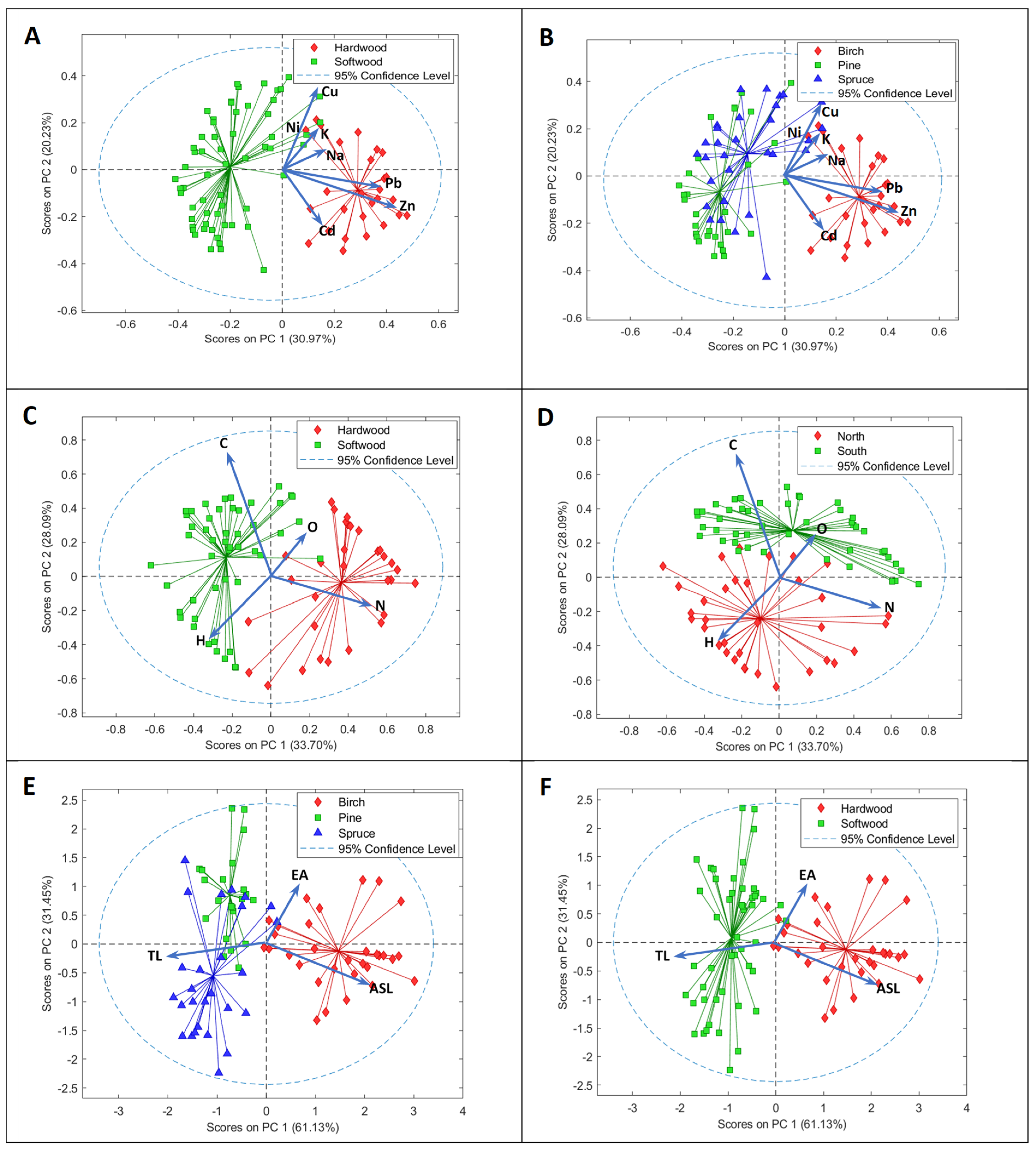
Figure 1. PCA of wood samples’ chemical data: (a,b)—metal contents; (c,d)—organic elements CHNO; (e,f)—biocomposition of wood. Blue arrows represent loading vectors for metals (a,b), organic elements (c,d) and biocomposition (e,f) (total lignin (TL), acid-soluble lignin (ASL), and extractives (EA)).
Analytica 06 00046 g001
Figure 2. ATR-FTIR spectra of birch, spruce, and pine woods.
Analytica 06 00046 g002
Figure 3. PCA analysis ATR-FTIR spectra of wood samples (a) and loadings profile of PC 2 (b).
Analytica 06 00046 g003
Figure 4. PLS-DA model showing discrimination of hardwood (class 1) from softwood (class 2).
Analytica 06 00046 g004
Table 1. Classes of wood samples used in the study.
ClassSub-ClassNumber of Samples
Wood speciesBirch32
Pine30
Spruce30
Wood typeHardwood32
Softwood60
Place of growthNorthern Estonia45
Southern Estonia47
Table 2. Characterization of wood samples by chemical methods.
BirchPineSpruce
Average ± SD (n = 32)Range (Min–Max)Average ± SD (n = 30)Range (Min–Max)Average ± SD (n = 30)Range (Min–Max)
Zn, mg/kg22.5 ± 10.79.0–445.1 ± 2.4 3.0–126.8 ± 4.1 3.0–21.3
Na, mg/kg4.6 ± 2.52.9–12.23.2 ± 1.03.0–8.23.3 ± 0.9 3.0–7.5
K, mg/kg349 ± 140182–777225 ± 118109–504456 ± 458158–1760
Cu, mg/kg0.88 ± 0.220.44–1.390.79 ± 0.350.34–2.110.94 ± 0.300.45–1.73
Pb, mg/kg0.69 ± 0.460.19–2.200.07 ± 0.020.05–0.280.22 ± 0.140.05–0.58
Cd, mg/kg0.08 ± 0.040.02–0.190.07 ± 0.040.01–0.160.05 ± 0.030.003–0.15
Ni, mg/kg0.05 ± 0.020.02–0.110.07 ± 0.030.04–0.350.07 ± 0.060.02–0.28
C %dw47.7 ± 1.743.2–49.249.6 ± 2.742.3–52.648.1 ± 3.337.4–50.4
H %dw6.5 ± 0.35.5–6.86.7 ± 0.36.0–7.16.5 ± 0.35.6–6.9
N %dw0.10 ± 0.020.1–0.20.07 ± 0.02 0.03–0.130.06 ± 0.020.04–0.12
O %dw46.8 ± 0.844.9–48.344.7 ± 1.640.4–46.945.9 ± 2.139.0–48.3
ASL %dw2.3 ± 0.71.3–3.60.45 ± 0.110.33–0.670.40 ± 0.100.32–0.60
TL %dw26.1 ± 2.421.1–30.532.1 ± 2.228.5–36.431.0 ± 2.2 26.4–35.7
EA %dw3.5 ± 0.82.1–5.06.1 ± 2.92.8–11.52.0 ± 0.70.9–4.0
SD—standard deviation, ASL—acid-soluble lignin, TL—total lignin, EA—extractives.
Table 3. Assignment of bands in the ATR-FTIR spectra of wood samples [5,19].
Wavenumber, cm−1Band Assignments
3335OH stretching in hydroxyl, hydrogen bonding
2927CH stretching in methyl and methylene groups
1735–1725C=O stretching in unconjugated ketone, carbonyl, and aliphatic groups of xylan
1640C=O stretching conjugated to aromatic ring
1592Aromatic skeletal vibration typical for S units plus C=O stretch
1508–1503C=C stretching in the aromatic ring
1457CH2 deformation stretching
1421Aromatic skeletal combined with C–H in-plane deforming and stretching
1370Aliphatic CH stretching in methyl group and phenol
1323Condensation of guaiacyl and syringyl units, CH2 bending stretching
1232C-O-C stretching of phenol-ether bond in lignin
1158C-O-C stretching in pyranose rings, C=O stretching in aliphatic groups
1030C=O deformation in alcohols, C-O stretch conjugation
895C-H stretching out of plane of aromatic ring
595C-H stretching, O-H bending
Table 4. Model performance for the discrimination of wood samples based on wood species, wood type, and place of growth using PLS-DA.
Data Cap. Var. %Modeled ClassSensitivity (cal)/(pred)Specificity (cal)/(pred)Class Error * (cal)/(pred)RMSECRMSECVRMSEP
FTIR, 3 LVs66.5Hardwood1.0/1.01.0/1.00/00.040.050.04
Softwood1.0/1.01.0/1.00/00.040.050.04
FTIR, 3 LVs62.7Birch1.0/1.01.0/1.00/00.050.060.06
Pine0.90/0.500.93/0.570.08/0.460.300.440.50
Spruce1.0/0.700.93/0.710.04/0.290.290.440.48
Organic elements, 3 LVs76.9Hardwood1.0/0.880.96/1.00.02/0.060.260.270.28
Softwood0.96/1.01.0/0.880.02/0.060.260.270.28
Organic elements, 3 LVs77.6North0.98/1.00.97/1.00.03/0.00.230.250.25
South0.98/1.00.97/1.00.03/0.00.230.250.25
Metals, 4 LVs72.7Hardwood0.86/0.910.93/1.00.11/0.040.240.260.25
Softwood0.93/1.00.86/0.910.11/0.040.240.26 0.25
Metals, 4 LVs (split Onion)73.3Birch0.91/0.910.95/0.910.07/0.090.230.250.25
Pine0.85/0.900.81/0.670.17/0.210.340.380.37
Spruce0.80/0.600.71/0.860.24/0.270.390.440.38
Biocomposition,
3 LVs
100Hardwood1.0/1.01.0/1.00/00.110.120.27
Softwood1.0/1.01.0/1.00/0 0.110.120.27
Biocomposition,
3 LVs
100Birch1.0/1.01.0/1.00/0.00.110.110.29
Pine0.98/0.500.83/0.780.04/0.250.240.260.46
Spruce0.90/0.900.75/0.720.07/0.500.300.310.57
* Class. Error = 1 − (sensitivity + specificity)/2 − average of false positive rate and false negative rate for class.
Table 5. The performance of partial least squares (PLS) models for the prediction of Klason lignin (KL), acid-soluble lignin (ASL), and extractives (EA) based on different wavenumber ranges.
ParameterModelNLVInterval (Variables)R2calRMSECRMSECVR2predRMSEPRPD
Klason lignin Full PLS5[1:3734]0.940.831.350.850.972.58
BiPLS6[1:100 301:500 601:800 901:1000 1101:1400 2101:2200 2401:2800 3001:3100 3201:3500 3601:3734]0.940.981.190.870.882.78
Acid-
soluble lignin
Full PLS7[1:3734]0.980.150.240.840.322.50
BiPLS7[1:100 401:500 701:800 1001:1100 1201:1300 1701:1800 2401:2500 3101:3200 3301:3400 3701:3734]0.990.140.290.860.302.67
ExtractivesFull PLS6[1:3734]0.990.171.510.800.982.24
BiPLS7[301:400 901:1400 2201:2300 2401:2500 2601:2700 3701:3734]0.990.190.710.850.652.58
Disclaimer/Publisher’s Note: The statements, opinions and data contained in all publications are solely those of the individual author(s) and contributor(s) and not of MDPI and/or the editor(s). MDPI and/or the editor(s) disclaim responsibility for any injury to people or property resulting from any ideas, methods, instructions or products referred to in the content.