GNSS and Mobile Network Data Fusion: Positioning Performance with DGNSS Methods

Abstract

A differential global navigation satellite system (DGNSS) improves the accuracy of conventional GNSS by utilizing reference stations to provide real-time correction data for positioning errors. In mobile networks, positioning methods based on signal parameters and location servers assist GNSS receivers by supplying correction information to mitigate errors from satellite clock inaccuracies, atmospheric disturbances, and orbital deviations. Depending on the configuration between the receiver and transmitter, base station and receiver clock errors are effectively eliminated. Proposed positioning algorithms leveraging mobile network observations in both coordinate and range domains demonstrate performance comparable to DGNSS solutions, offering a viable alternative for positioning in GNSS-denied environments. Experimental evaluations are conducted in outdoor scenarios under static conditions to validate the approach.

1. Introduction

Global navigation satellite systems (GNSSs) determine a user’s position by measuring the distance between a receiver and multiple satellites through trilateration. This technique requires signals from a minimum of four satellites to compute the receiver’s latitude, longitude, altitude, and time. However, the accuracy of these measurements is degraded by several error sources, including orbital inaccuracies, satellite and receiver clock biases, ionospheric and tropospheric delays, multipath, and noise [1] (p. 279). The impact of these errors depends strongly on satellite geometry, typically expressed by a dilution of precision (DOP) factor that expresses how satellites’ geometry amplifies measurement errors into position errors. The combination of these error sources typically limits the accuracy of a standalone GNSS for consumer-grade receivers to about 5–10 m under open-sky conditions. In dense urban environments, where multipath and no-line-of-sight (NLOS) effects dominate, accuracy degradation can exceed 20 m, and in GNSS-denied scenarios such as tunnels, underground facilities, or areas with severe signal blockage, positioning may become unavailable. To mitigate errors, the implementation of advanced positioning techniques such as differential GNSS (DGNSS), real-time kinematic (RTK), and precise point positioning (PPP) is commonly used. These methods apply correction data derived from ground-based reference stations, continuously operating reference station (CORS) networks, or precise atmospheric and orbital models. PPP, although globally applicable and independent of local reference stations, requires several minutes of convergence time to achieve sub-decimeter accuracy.

In contrast, RTK is a high-precision GNSS positioning technique that uses correction data from a fixed base station with a precisely known position, computing the error and transmitting correction data to the rover [2]. RTK delivers centimeter-level precision based on carrier-phase measurements and resolving integer ambiguities. RTK typically requires dual-frequency GNSS receivers and shorter distances within 30 km of a reference station [3] (p. 400). RTK is more complex, involving robust communication links and real-time correction using transmission protocols such as RTCM [4]. RTK is now being explored for consumer-grade equipment such as smartphones, which take advantage of their multi-frequency and multi-constellation GNSS capabilities.

In DGNSS, single and double differences are essential techniques for mitigating common errors such as satellite and receiver clock biases. Single differences (SDs) calculate the difference between measurements from two receivers or two satellites to remove errors such as satellite clock biases or receiver clock errors, while double differences (DD) use the difference between two single differences, eliminating both satellite and receiver clock biases simultaneously, achieving robust, centimeter-level accuracy [1] (pp. 469–486). These differential techniques form the basis for high-accuracy GNSS positioning, reducing common errors and providing a robust framework that can also be adapted to other positioning domains.

While GNSS remains the primary technology for global positioning, its performance is often degraded or unavailable in urban canyons, tunnels, or indoor environments. In such cases, mobile networks provide an alternative or complementary positioning service exploiting the existing cellular infrastructure to estimate the user’s location. Network-based positioning utilizes the observation and measurement of radio signal parameters exchanged between user equipment (UE) and surrounding base stations (BTSs). Techniques such as time of arrival (TOA), time difference of arrival (TDOA), round-trip time (RTT), angle of arrival (AoA), and cell ID exploit temporal and spatial properties of the received signals. These measurements are managed by dedicated positioning servers, which play a central role in mobile network–based localization, as they collect, process, and store all relevant information to deliver accurate position estimates.

Depending on the service, the servers can provide assisted GNSS (A-GNSS), cellular positioning, or hybrid GNSS–network solutions. An A-GNSS transmits satellite corrections and ephemeris data to reduce the time to first fix (TTFF) and mitigate errors from satellite clocks and atmospheric delays. Cellular positioning applies network-based methods such as TOA, TDOA, and others, while hybrid positioning integrates GNSS with terrestrial signals from cellular, Wi-Fi, or Bluetooth networks. Additionally, high-precision servers that provide RTK/PPP corrections [5] (p. 179) are often available as paid services. The role of these servers is to enhance positioning performance in challenging scenarios and to manage and process data that is regularly inaccessible to common mobile users, who only receive the final estimated position.

The particular case of A-GNSS can be considered a practical extension of the DGNSS concept, since it also relies on external infrastructure (mobile networks) to provide correction and assistance data to GNSS receivers. This approach improves positioning accuracy by addressing satellite clock errors, orbital deviations, coarse-time assistance, and atmospheric delays. According to the 3GPP technical specification TS 38.171 [6], A-GNSS UE must meet minimum performance requirements when valid assistance data are available to perform GNSS measurements and position calculations. The specification does not consider delays, but it defines that under multipath conditions, the 2D position error shall not exceed 100 m with a maximum of TTFF of 20 s [6] (p. 20). A-GNSS requires an active internet connection to obtain this assistance data.

While mobile networks provide valuable assistance for GNSS positioning, their effectiveness is constrained by the need for continuous connectivity. In situations where internet access is limited or unavailable, such as in remote areas, tunnels, or GNSS-denied environments, alternative approaches are required. One viable alternative is the use of traditional techniques such as relative positioning.

The concept of relative positioning, widely used in GNSS, depends on the geometry between the satellite and the receivers. By forming combinations of pseudorange and carrier-phase measurements, it is possible to remove errors such as satellite and receiver clock bias or atmospheric delays. This same principle can be applied in mobile networks, where the BTS assumes the role of satellites and the UE acts as the receiver. Applying SD and DD to the measurements between BTS and the UE can reduce common errors such as device clock bias and network synchronization offsets, leading to more accurate positioning. In both GNSS and mobile networks, geometry and the cancellation of shared errors are the key elements for improving positioning accuracy.

In GNSS, relative positioning is typically used to determine the vector, or baseline, between two points, where one of them is fixed and the other unknown, by performing simultaneous observations from two receivers to at least two satellites at the same epoch. From these observations, linear combinations are formed to cancel systematic errors. For example, subtracting pseudoranges in SD between receivers reduces ionospheric and tropospheric delays, which in short baselines, can otherwise reach tens of meters. DD extends this process by also cancelling both satellite and receiver clock errors, making it possible to reach centimeter-level precision, especially in static applications.

Analogously, in a mobile network, SDs are calculated by determining the timing or signal differences between two base stations observing the same device. This process effectively eliminates device clock biases and reduces synchronization errors, providing a more accurate representation of the signal transmission. DD extends this concept by comparing the SD obtained across multiple BTSs or devices, improving consistency and robustness. These methods are widely applied in positioning systems such as TDOA and AoA, particularly in 4G and 5G networks. However, challenges such as the need for highly synchronized base stations, susceptibility to noise in dense urban environments, and reliance on optimal network geometry can limit their effectiveness.

Accessing A-GNSS services is not straightforward, as it involves restrictions related to permissions, communication protocols, and network connectivity. The information processed by mobile network positioning servers is generally not accessible to end-users. To address this limitation, several tools and applications have been developed that interact with cellular towers and positioning servers, enabling the extraction of raw measurements and positioning-related data.

In parallel, in May 2016, Google released access to raw GNSS measurements through the Android location application programming interface (API), including pseudorange, carrier-phase, and Doppler data [7]. This innovation opened new opportunities for researchers, enabling the development of advanced positioning techniques using consumer-grade devices.

At the same time, smartphones have undergone significant evolution in their hardware capabilities. Modern devices integrate multi-constellation and dual-frequency GNSS chipsets, capable of tracking GPS, Galileo, GLONASS, and BeiDou signals simultaneously, including modern bands such as GPS L5 and Galileo E5. Although the small size and low gain of smartphone antennas still introduce higher noise and multipath susceptibility compared to geodetic-grade equipment, advances in antenna design, signal processing, and sensor integration have greatly improved measurement quality. Importantly, these GNSS improvements are complemented by hybrid positioning strategies, where data from GNSS is fused with observations from cellular networks, Wi-Fi, Bluetooth, and embedded sensors. By combining barometers, inertial measurement units (IMUs), and network-based assistance, smartphones achieve greater robustness and continuity, reaching sub-meter or even centimeter-level positioning in favorable conditions. As a result, they have become powerful hybrid platforms for precision applications that were once limited to professional-grade equipment.

The Xiaomi Mi 8 has become a reference device in the scientific community for precise positioning research. As the first commercial smartphone capable of recording dual-frequency GNSS signals, carrier-phase measurements, and multiconstellation [8], it provided the necessary conditions for applying advanced techniques, such as RTK and DGNSS, with sub-meter or even centimeter-level accuracy. Following its release, numerous studies and publications adopted Xiaomi Mi 8 as an experimental platform, making it a de facto benchmark for evaluating the feasibility of precise positioning with consumer devices. Although more recent smartphones, such as the Huawei P30 Pro or later Xiaomi models, also include dual-frequency capabilities, the Xiaomi Mi 8 remains the foundational reference in the literature. This makes it an ideal starting point for methodological developments, which can then be extended to other devices with similar characteristics.

In addition to the hardware capabilities demonstrated by Xiaomi Mi 8, precise smartphone positioning also relies on the external services and communication protocols that provide correction and assistance data. Prominent examples include SUPL (secure user plane location), which supports A-GNSS data transmission, NTRIP (networked transport of RTCM via internet protocol) for delivering high-precision corrections, and Google’s fused location API [9], which combines satellite, cellular, and Wi-Fi signals to offer robust and reliable location services. Together, these technologies complement the hardware improvements and form the operational framework that enables smartphones to achieve high-accuracy positioning comparable to professional-grade GNSS receivers. Within this technological context, several studies have been conducted to evaluate the actual performance of smartphones and to validate the feasibility of precise positioning using these capabilities.

For example, in [10], RTK is applied to smartphone GNSS data, which is fused with IMU sensors, to achieve centimeter-level positioning accuracy. It highlights challenges like multipath interference and low-quality antennas but demonstrates improvements with choke-ring platforms. These findings are consistent with the comprehensive antenna characterization presented in [11], where Xiaomi Mi 8 GNSS L1/L5 antennas were experimentally evaluated under the geodetic GNSS antenna calibration methodology. The study determined that the device integrates two planar inverted-F (PIFA) microstrip antennas, located at the upper part of the smartphone, operating at 1.575 GHz (L1/E1/B1) and 1.176 GHz (L5/E5a/B2a). Laboratory measurements in an anechoic chamber and complementary outdoor tests revealed omnidirectional radiation patterns with low directivity and no gain with respect to an isotropic antenna. Such a pattern enables signal reception from any direction but also makes the antenna highly susceptible to noise and multipath reflections, particularly in urban or obstructed environments. The experiment further demonstrated that the use of metallic shielding structures significantly modifies the radiation pattern, reducing multipath interference and improving RTK precision by nearly an order of magnitude. This detailed analysis confirmed that antenna geometry and radiation behavior are major limiting factors in achieving geodetic-grade positioning performance with smartphones. In [12], the quality of GNSS observations from recent Android smartphones, such as Huawei P30 and Xiaomi Mi 8, and their potential for precise positioning using multi-GNSS signals are analyzed. The study evaluates signal noise, satellite tracking capability, and phase observations for achieving centimeter-level accuracy in smartphone-to-smartphone relative positioning. In [13], the feasibility of centimeter-level RTK positioning using dual-frequency GNSS chipsets in smartphones is investigated, focusing on the Xiaomi Mi 8. The study evaluates two configurations between a geodetic receiver as the master and a smartphone as the rover, with both the master and rover being smartphones. The results improved positioning precision with dual-frequency GNSS (L1 + L5), achieving 2D accuracy of 2–3 cm and sub-meter vertical accuracy in ideal conditions. In [14], an RTK positioning system for smartphones is proposed to address low positioning accuracy in GNSS-based smartphone navigation. The system integrates a GNSS reference station, an NTRIP system, and smartphones to achieve high-accuracy positioning. As a result, RTK positioning reduced longitudinal error to 0.83 m and latitudinal error to 0.79 m compared to standard GNSS results of 1.94 and 3.11 m, respectively. In contrast, DGNSS uses pseudorange corrections from a base station to achieve meter-level accuracy and can operate over longer baselines of up to 300 km with single-frequency receivers [15]. DGNSS, being simpler and more cost-effective, has broader accessibility but lacks the precision of RTK. DGNSS provides meter-level accuracy by applying pseudorange corrections from a base station, typically via RTCM protocols transmitted over cellular or internet networks. Some research analyzes the accuracy of DGNSS positioning using dual-frequency pseudorange measurements (L1 and L5) from Huawei P30 Pro smartphones. The results show that utilizing the L5 frequency significantly improves positioning accuracy compared to the L1 frequency, achieving errors as low as 0.3 m. In [16], a neural network designed to mitigate biased errors in pseudoranges is introduced, enhancing localization performance with data collected from mobile phones. The corrected pseudoranges are utilized by a model-based localization engine to compute more accurate positions.

Recent research has explored the feasibility of achieving high-accuracy positioning with consumer-grade smartphones, particularly after the release of dual-frequency GNSS chipsets and access to raw measurements through the Android API. Reviewing these contributions is essential for understanding the current state of smartphone positioning, highlighting the experimental evidence obtained so far, and identifying the limitations that remain to be addressed. The availability of raw GNSS measurements in Android devices and the integration of dual-frequency chipsets have motivated a large body of research on precise smartphone positioning. Several studies have investigated the feasibility of applying classical GNSS techniques, such as RTK and DGNSS, with consumer devices, while others have explored the use of machine learning and hybrid approaches. These works provide experimental evidence of the current capabilities and limitations of smartphones in achieving sub-meter or even centimeter-level accuracy. Representative contributions from the literature are summarized in the following Table 1.

Table 1. Overview of related works addressing precise positioning techniques using smartphone GNSS measurements.

Ref.	Device(s) Tested	Objective	Methodology	Accuracy Results	Environment	Limitations	Relation to This Work
[6] ETSI TS 138 171 V15.1.0 (2019-05) (2019)	Android smartphone + onboard IMU	Demonstrate fused RTK + inertial positioning using only smartphone sensors	Fusion of GNSS raw data and IMU in RTK framework	cm-level	Controlled tests	Requires IMU integration, complexity in processing	Shows potential for high precision but adds complexity; our method avoids IMU reliance
[7] European GNSS Supervisory Authority (2017)	Huawei P30, Xiaomi Mi 8	Analyze quality of multi-GNSS observations	Assessment of noise, tracking, carrier phase; smartphone-to-smartphone relative positioning	cm-level	Open-sky and urban	Noise, multipath sensitivity	Confirms feasibility of raw GNSS in smartphones; supports measurement analysis
[8] European Union Agency for Space Program World’s First Dual-Frequency GNSS Smartphone Hits the Market (2024)	Xiaomi Mi 8	Evaluate dual-frequency RTK feasibility	Single-baseline RTK with dual-frequency chipset	2–3 cm 2D, <1 m vertical	Ideal, open-sky	Poorer vertical accuracy, antenna limits	Establishes Xiaomi Mi 8 as reference device for dual frequency; our method builds upon this
[9] Android Developers (Google)	Android smartphones + GNSS reference station	Implement RTK system for smartphones	Use of NTRIP corrections integrated with smartphones	Errors reduced to ~0.8 m vs. 2–3 m in standalone GNSS	Urban	Requires external reference and correction service	Demonstrates correction benefits; analogous to our hybrid approach with network assistance
[10] Bochkati et al. (2020)	General GNSS receivers (theoretical)	Explain DGNSS principle	Base station pseudorange corrections up to 300 km	~1 m accuracy	Theoretical, generalized	Lower precision than RTK; needs correction data	Provides theoretical basis; foundation for adapting DGNSS to mobile networks
[11] Haro et al. (2024)	Huawei P30 Pro (dual frequency)	Assess DGNSS accuracy with L1 vs. L5	Compare pseudorange corrections on L1 vs. L5	0.3 m with L5 vs. higher errors with L1	Urban/mixed	Smartphone antenna limitations	Shows clear benefit of dual frequency; relevant for our approach
[12] Paziewski et al. (2021)	Various Android smartphones	Improve GNSS positioning with machine learning	Neural network (PrNet) to correct pseudorange biases	Improved localization accuracy with corrected pseudoranges	Field data	Dependent on ML model and training data	Demonstrates potential of AI corrections; complementary to our differential approach

This work proposes to develop the relative positioning differential (RPD) algorithm to determine the incremental components of the vector between base and rover, based on the weighted least square (WLS) position solution, using mobile networks and GNSS observation data. RPD adopts the basic principle of DGNSS, where two receivers, a base and a rover, are involved in both smartphones. They receive the horizontal position estimate coordinates expressed in latitude/longitude from the mobile network through the geolocation API [17] while simultaneously collecting GNSS observation data.

The proposed algorithm is based on two different levels of positioning strategies in accordance with the authors of [18]. The position-level method combines independent positions (UE coordinates: base and rover) obtained directly from the mobile network and GNSS, and the measurement-level method is based on ranging measurements between UE and BTS, which are not directly available and must be computed, and pseudorange measurements between UE and GNSS satellites. Observation data from the mobile network is obtained using the GnssLogger App (version 3.1.0.7, GnssLogger App: Company: Google LLC, City: Mountain View, State: CA, Country: USA) [19], and GNSS pseudorange measurements are collected using the Geo++ Rinex Logger (version 2.1.8, Company: Geo++ GmbH, City: Garbsen, State: N/A, Country: Germany) [20].

The paper is organized as follows. Section 2 describes the materials and methods of the mobile network RPD algorithm positioning models. In Section 3, the performance of the proposed methods is evaluated with numerical experiments. Finally, Section 4 discusses the obtained results and their implications.

2. Materials and Methods

The development of the RPD methods is based on BTS fix coordinates and UE’s (base and rover) coordinates obtained from mobile network and GNSS receiver, in outdoors environment and static position. The proposed analysis relies on the fact that WLS is applied in a single epoch to a set of n observations to estimate the user’s (rover) relative position. Both RPD methods have been developed in Python (version 3.10.12 Company: Python Software Foundation, City: Beaverton, State: OR, Country: USA). In the position-level RPD, the coordinate domain is used, and for measurement-level RPD, the network ranges are computed indirectly, since they are not available from the network. GNSS pseudoranges’ data were processed using RTKlib (version 2.4.3 b34, Tomoji Takasu, RTKLIB Open Source Project, Tokyo, Japan). The coordinates of the BTSs surrounding the test area were obtained from Spain’s official mobile network repository through its website [21] and checked with a Trimble Total Station and professional Leica GNSS equipment. The UE (base and rover) coordinates’ reference points are computed with a professional-grade Leica System 1200 device. The positions and coordinates of the BTS, base, and rover are presented in Figure 1 and Table 2 and Table 3.

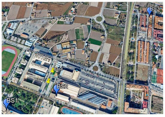
Figure 1. Base stations’ mobile network (BTS1, BTS2, BTS3) and base and rover smartphones.

Table 2. Reference base and rover vertex coordinates.

UE	E (m)	N (m)	U (m)	${\mathsf{\sigma }}_{\mathit{E}}$ (m)	${\mathsf{\sigma }}_{\mathit{N}}$ (m)	${\mathsf{\sigma }}_{\mathit{U}}$ (m)
Base	729,063.06	4,373,540.22	55.52	0.03	0.01	0.04
Rover	729,042.49	4,373,478.17	55.65	0.02	0.03	0.05

Table 3. Base station mobile network vertex coordinates.

#	E (m)	N (m)	U (m)	${\mathsf{\sigma }}_{\mathit{E}}$ (m)	${\mathsf{\sigma }}_{\mathit{N}}$ (m)	${\mathsf{\sigma }}_{\mathit{U}}$ (m)
BTS1	728,856.17	4,373,346.20	93.22	0.03	0.02	0.04
BTS2	729,094.42	4,373,423.43	72.07	0.01	0.03	0.05
BTS3	729,592.05	4,373,891.14	82.22	0.02	0.02	0.05

The experiments were conducted using two Xiaomi Mi 8 smartphones, the first commercial devices to support dual-frequency GNSS and carrier-phase measurements. Although this model was released in 2018, it remains widely adopted in the scientific community as a reference for precise smartphone positioning. Its Qualcomm SDM845 chipset enables consistent acquisition of raw GNSS and network-based measurements. Hardware variability across smartphone models may influence performance; however, the use of Xiaomi Mi 8 provides a baseline representative of the general behavior of consumer-grade devices, which commonly employ microstrip PIFA microstrip antenna.

Consequently, all data acquisition is performed via Android’s geolocation and GNSS measurement APIs: GnssLogger supplies network-assisted position estimates and timing information, while Geo++ RINEX Logger provides raw GNSS observations (RINEX 3.x) for differential processing. Both tools interface directly with the Android geolocation API, which interacts directly with the cellular radio bases to obtain position estimates and network-derived location data.

Since direct access to the internal databases of mobile network positioning servers is not permitted for end-users, these APIs provide the only available interface for accessing and analyzing network-assisted geolocation information. The raw data collected through these interfaces were processed using DGNSS to evaluate the precision of the mobile network positioning. During the observed time, the coordinates (latitude, longitude, and altitude) and accuracy values are recorded simultaneously, one epoch at a time. Both apps operate in the background without interrupting each other. The base and rover receivers do not exhibit correlated noise; in other words, their variances are independent, since the phones are physically separated by a short baseline and exposed to different environments. We implement the RPD algorithm to estimate the base–rover baseline. Figure 2 outlines the pipeline, which includes preprocessing, position-level and measurement-level branches, RPD with WLS, and statistical evaluation. Full details are provided in Section 2.1 and Section 2.2.

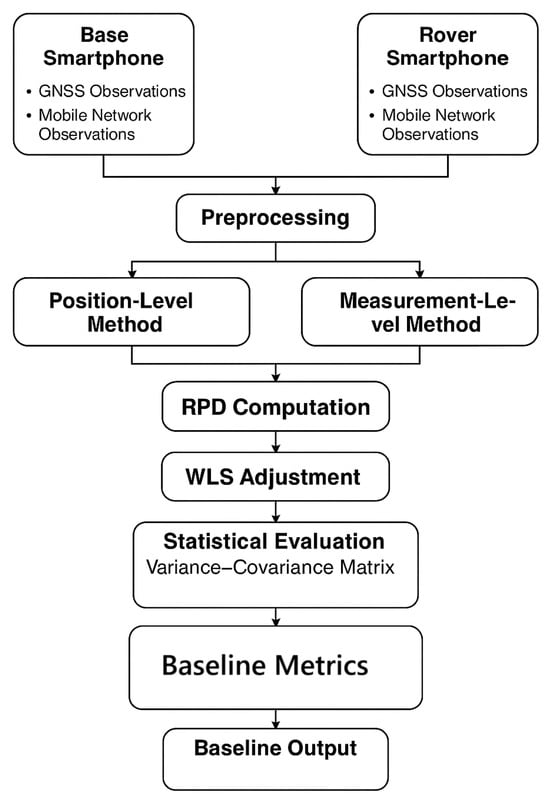
Figure 2. Workflow of RPD algorithm for base–rover baseline and coordinates’ estimation from GNSS and mobile network observations.

2.1. Position-Level RPD Method

This method computes the increment coordinates between two smartphones established as base and rover using the coordinates observed from the mobile network. It uses the adjustment specified in the theory of the deterministic Gaussian method [22] to determine the rover’s relative position.

The rover and base register their coordinates, as shown in Equation (1) by t epoch for n observations. In Equations (2)–(4) and (6), the mathematical models are designed to compute the value for each component (x, y, z) for n observations, which is represented by an identity matrix $I_3$.

$$I_3={\left[\begin{array}{ccc}1& 0& 0\\ 0& 1& 0\\ 0& 0& 1\end{array}\right]}_{3\times 3}$$

where the diagonal represents each component (x, y, z).

So, the coordinates’ vectors of the base and rover are:

$${P_{base}^{\left(t\right)}=\left[\begin{array}{c}{x}_b^{\left(t\right)}\\ y_b^{\left(t\right)}\\ z_b^{\left(t\right)}\end{array}\right]}_{3\times 1},{P_{rover}^{\left(t\right)}=\left[\begin{array}{c}{x}_r^{\left(t\right)}\\ y_r^{\left(t\right)}\\ z_r^{\left(t\right)}\end{array}\right]}_{3\times 1}$$

(1)

Using the mathematical model represented in an observation equations system [23] with n observation epochs, a WLS solution is applied. The matrix form of the mathematical model is well defined in [24,25], and it can be expressed in terms of the matrix as:

$$Ax=b+\upsilon$$

(2)

$$A={\left[\begin{array}{c}{I}_3\\ I_3\\ ⋮\\ I_3\end{array}\right]}_{3n\times 3},x={\left[\begin{array}{c}\begin{array}{c}dx\\ dy\end{array}\\ dz\end{array}\right]}_{3\times 1},b={\left[\begin{array}{c}∆P_{obs}^{\left(1\right)}\\ \begin{array}{c}∆P_{obs}^{\left(t\right)}\\ ⋮\end{array}\\ ∆P_{obs}^{\left(n\right)}\end{array}\right]}_{3n\times 1},\upsilon =\mathrm{residuals}$$

where:

• The coefficients of the design matrix $A$ correspond to the identity matrix of n observations.
• Coordinates’ vector $x$ of the variable’s coordinates of m variables is unknown.
• Vector of independent terms $b$ contains increment coordinates between the base and rover for n observations at each t epoch.
• $∆P_{obs}^{\left(t\right)}=P_{rover}^{\left(t\right)}-P_{base}^{\left(t\right)}$.
• $\upsilon$ is the vector of residuals.

The use of stacked $I_3$ blocks provide a compact representation of the linear relationship between the coordinate corrections $\left(dx,dy,dz\right)$ and each three-dimensional observation. Specifically, each observation vector is expressed in Equation (2), ensuring that the same correction applies directly to all coordinates.

Applying WLS method assigns specific weights to each equation. Consequently, the mathematical model Equation (2) can be computed using observations as follows:

$$W\left(Ax\right)=W(b+\upsilon )$$

(3)

where $W$ is the diagonal weight matrix of n observations, and it is represented in Equation (4):

$$W={\begin{array}{c}\left[\begin{array}{cccc}{w}_1{I}_3& 0& \dots & 0\\ 0& w_2{I}_3& \dots & 0\\ ⋮& ⋮& \ddots & ⋮\\ 0& 0& \dots & w_n{I}_3\end{array}\right]\\ \end{array}}_{3n\times 3n}$$

(4)

The diagonal elements of the matrix $W$ are a function of the accuracy value provided by the GNSSLogger app.

$$w_n={\displaystyle \frac{1}{{\sigma }_n^2}}$$

(5)

where:

• ${\sigma }_n^2={\displaystyle \frac{{\sigma }_0^2}{{\sigma }_{base,n}^2+{\sigma }_{n,\mathrm{r}\mathrm{o}v\mathrm{e}\mathrm{r}}^2}}$.
• ${\sigma }_0^2$ is a constant variance value.

The WLS solution for vector $x$ is:

$$x={{(A}^{T}WA)}^{-1}{A}^{T}Wb$$

(6)

The vector $x$ in Equation (6) will give us the adjusted increments as follows:

$$∆P_{adjusted}=∆P_o+x$$

(7)

where:

• $∆P_o$ is the vector with initial values $∆P_o={\left[\begin{array}{c}∆x_o\\ ∆y_o\\ ∆z_o\end{array}\right]}_{3\times 1}$.

So:

$$∆P_{adjusted}={\left[\begin{array}{c}∆x_{adjusted}\\ ∆y_{adjusted}\\ ∆z_{adjusted}\end{array}\right]}_{3\times 1}={\left[\begin{array}{c}∆x_o\\ ∆y_o\\ ∆z_o\end{array}\right]}_{3\times 1}+{\left[\begin{array}{c}\begin{array}{c}dx\\ dy\end{array}\\ dz\end{array}\right]}_{3\times 1}$$

and the Euclidean norm:

$$d=‖∆P_{adjusted}‖=\sqrt{{{∆x}_{adjusted}}^2+{∆y_{adjusted}}^2+{∆z_{adjusted}}^2}$$

(8)

and for residual $\upsilon$ vector, it is:

$$\upsilon =Ax-b$$

(9)

According to the accuracy desired and selected by the user, a threshold in Equation (10) is established based on the values of the independent term $b$ to remove outliers or blunders in observed data:

$$\left|\upsilon \right|>p\left|{\upsilon }_{all}\right|$$

(10)

where $\upsilon$ is the residual calculated from Equation (9), and ${\upsilon }_{all}$ is the mean of all residuals. Restrictive value parameter is denominated $p$; for example, $p=1.5$.

The variance–covariance matrix $\Sigma$ provides the accuracy of the WLS solution:

$$\Sigma ={{\sigma }_{0P}^2{(A}^{T}WA)}^{-1}$$

(11)

where the a posteriori variance factor of unit weight ${\sigma }_{0P}^2$ is:

$${\sigma }_{0P}^2={(\upsilon }^{T}P\upsilon )/(3n-m)$$

(12)

where:

• n is the number of observations, and m is the number of unknown variables.

The diagonal elements of the variance–covariance matrix $\Sigma$ are ${\sigma }_{xx}^2$, ${\sigma }_{yy}^2$, and ${\sigma }_{zz}^2$ and represent the standard errors in east, north, and up (ENU) local coordinate system. The standard deviations ${\sigma }_x$, ${\sigma }_z,$ and ${\sigma }_z$ assess and compare the positioning performance of RPD GNSS and mobile network positioning to select the most accurate method.

$${\sigma }_x=\sqrt{{\sigma }_{xx}^2},{\sigma }_y=\sqrt{{\sigma }_{yy}^2},{\sigma }_z=\sqrt{{\sigma }_{zz}^2}$$

(13)

2.2. Measurement-Level RPD Method

This RPD method is based on relative positioning between the range of the BTS and one or more rovers and pseudorange between GNSS satellites and rovers in SD and DD configurations. The range between the BTS and UE is not directly available from the mobile network. It is computed using the Euclidean norm (8).

2.2.1. Single-Difference Method (SD)

Differential techniques involve comparing measurements from multiple receivers to reduce common errors. The classical DGNSS algorithm is based on the SD of pseudorange observables; at a common epoch, and for a specific satellite, the simplified pseudorange observation equation is the following:

$$R_r^s={\rho }_r^s+{d\rho }_r^s+c\left({dt}_r-{dt}^s\right){+I}_{R_r^s}{+T}_{R_r^s}{+dm}_{R_r^s}+E_{rel}+r_{tn}$$

(14)

where:

• ${\rho }_r^s$ is the observed distance between the receiver r in reception time and the satellite s in transmission time.
• ${d\rho }_r^s$ is the linearizing of the satellite–receiver geometric range.
• $c$ is the speed of light.
• ${dt}_r$ is the receiver clock error.
• ${dt}^s$ is the satellite clock error.
• $I_{R_r^s}$ is the ionospheric delay on the GNSS signal.
• $T_{R_r^s}$ is the tropospheric delay on the GNSS signal.
• ${dm}_{R_r^s}$ is the multipath error for the pseudorange.
• $E_{rel}$ is the relativistic error.
• $r_{t_n}$ are residual errors.

The SD method is obtained by subtracting simultaneous pseudorange or carrier-phase observations from two receivers (base and rover) tracking the same satellite. The functional objective is to remove error terms that are common to both receivers.

In this operation, the satellite clock error is completely cancelled, since it affects both receivers in the same way. In the SD, several error sources remain even after differencing. The receiver clock bias remains present, as each receiver relies on its own oscillator. Satellite orbit errors are only slightly reduced because both receivers share a similar satellite geometry. Atmospheric effects, such as ionospheric and tropospheric delays, are only partially cancelled when the baseline is short, as the propagation conditions are highly correlated; however, for longer baselines, this correlation weakens, and significant residuals persist. Finally, multipath and receiver noise are specific to each receiver and therefore remain unaffected by the differencing process. To ensure effective error reduction, the baseline length between receivers should remain short. Other errors, such as receiver clock, orbit modeling, multipath, and thermal noise, are local errors that require additional strategies.

Analogously, in the mobile network, the single-difference method can be understood by considering two receivers (base and rover) connected to the same base station (BTS) at the same epoch. Here, the pseudorange is replaced by the measured range between the BTS and the UE. In cellular positioning, this range is typically estimated from ToA of the signal, or from TDoA/OTDoA techniques, which conceptually play the same role as pseudoranges in GNSS. The main error sources in mobile networks differ from those in GNSS. Ionospheric and tropospheric errors are not considered, since the standard BTS antenna height is approximately 25 m for a macrocell, with a maximum coverage radius of about 500 m [26] (p. 22). At this scale, signal propagation does not reach the ionospheric or tropospheric layers; therefore, these atmospheric effects are negligible. Instead, the dominant error is multipath, particularly under NLoS conditions, where the signal is reflected before reaching the UE. Additional error sources include the BTS clock bias, the UE clock bias, inaccuracies in BTS geometry or antenna calibration, and computational errors in the location server database. When two receivers are connected to the same base station (BTS) and perform simultaneous measurements toward it, forming the SD cancels the BTS clock bias because this term is identical in both observations. This situation is analogous to the SD GNSS.

In the cellular domain, this assumption is reinforced by the inherent synchronization architecture of the network. Each UE aligns its internal modem clock to the frame timing broadcast by the BTS, defined in LTE by the primary and secondary synchronization signals (PSSs/SSSs) within the 10 ms radio frame structure, and in 5G NR by the synchronization signal block (SSB). This process ensures that all UEs connected to the same cell share a common temporal reference derived from the BTS’s GNSS-disciplined clock. In addition, the network applies a timing advance (TA) adjustment to each UE, which compensates for individual propagation delays so that uplink transmissions arrive time-aligned at the BTS without modifying the frame timing reference itself. Therefore, two smartphones connected to the same BS are effectively synchronized to the same time base. Although each device has its own temperature-compensated crystal oscillator (TCXO), their clocks are disciplined by the same network timing source, using identical models and oscillator characteristics. Under these conditions, the differential receiver clock bias $\left({dt}_r\right)$ becomes negligible, allowing the SD to omit explicit time-bias estimation. The remaining residuals are dominated by uncorrelated effects, such as multipath, antennas, and hardware calibration differences, or small modeling errors in the BTS geometry or location server database.

The simplified range observation equation between BTS and UE (base or rover) is the following:

$$R_{UE}^{BTS}={\rho }_{UE}^{BTS}+{d\rho }_{UE}^{BTS}+c\left({dt}_{UE}-{dt}^{BTS}\right)+e_{UE}^{BTS}$$

(15)

where:

• The receiver r can be rover or base.
• ${\rho }_{UE}^{BTS}$ is the distance between the UE (base or rover) in reception time and the base station in a specific epoch.
• ${d\rho }_{UE}^{BTS}$ is the linearizing of the base station–receiver geometric range.
• $c$ is the speed of light.
• ${dt}_{UE}$ is the receiver clock error.
• ${dt}^{BTS}$ is the base station clock error.
• $e_{UE}^{BTS}$ is the multipath error for the Euclidean distance due to NLoS.

In a measurement-level method for mobile networks, only 2D positioning is computed, mainly because all base stations are at the same altitude, the design matrix A is singular [5] (p. 234), and the equation system cannot be solved. For this reason, in many real-life scenarios, only 2D positioning is possible. The altitude information must be obtained from other technologies as a barometer integrated in a smartphone [27]. The z coordinate is not considered to be an RPD network-based algorithm.

Then, the linearizing of the base station–receiver geometric range is as follows:

$${d\rho }_{UE}^{BTS}=\left[{\displaystyle \frac{x_{UE}-x^{BTS}}{{\rho }_{UE}^{BTS}}}\right]dx+\left[{\displaystyle \frac{y_{UE}-y^{BTS}}{{\rho }_{UE}^{BTS}}}\right]dy$$

(16)

where:

• $l_x^{BTS}=\left[{\displaystyle \frac{x_{UE}-x^{BTS}}{{\rho }_{UE}^{BTS}}}\right]; l_y^{BTS}=\left[{\displaystyle \frac{y_{UE}-y^{BTS}}{{\rho }_{UE}^{BTS}}}\right],$ and base station and receiver geocentric position are ${(x}^{BTS},y^{BTS})$ and ($x_{UE},y_{UE}$).

And the RPD-SD is:

$${}_{r}R_b^{{BTS}_n}=R_r^{{BTS}_n}-R_b^{{BTS}_n}$$

(17)

• n is the number of visible base stations with reachable coverage area.
• $R_r^{{BTS}_n}$ and $R_b^{{BTS}_n}$ are the Euclidean norm between base station and UE (base or rover).

Resolving the difference:

$$\begin{array}{c}{R}_r^{BTS} ={\rho }_r^{BTS}+{d\rho }_r^{BTS}+c\left({dt}_r-{dt}^{BTS}\right)+e_r^{BTS}\\ {-R}_b^{BTS} ={-\rho }_b^{BTS}-{d\rho }_b^{BTS}-c\left({dt}_b-{dt}^{BTS}\right)-e_b^{BTS}\end{array}$$

$$R_r^{BTS}{-R}_b^{BTS}={\rho }_r^{BTS}{-\rho }_b^{BTS}+{d\rho }_r^{BTS}-{d\rho }_b^{BTS}+c\left({dt}_r\right)-c\left({dt}_b\right)-{dt}^{BTS}+{dt}^{BTS}+e_r^{BTS}-e_b^{BTS}$$

The RPD-SD results in Equation (18):

$$R_r^{BTS}{-R}_b^{BTS}={\rho }_r^{BTS}{-\rho }_b^{BTS}+{d\rho }_r^{BTS}-{d\rho }_b^{BTS}+e_r^{BTS}-e_b^{BTS}$$

(18)

The SD observation equations can be expressed in a linearized form that relates the differential pseudorange measurements to the baseline vector between the two receivers. To estimate the unknown parameters, a WLS adjustment is applied as in Equation (2):

$$A={\left[\begin{array}{c}\begin{array}{c}\begin{array}{cc}{l}_{x_{1_{rov}}}^{{BTS}_1}& l_{y_{1_{rov}}}^{{BTS}_1}\end{array}\\ \\ ⋮\end{array}\\ \begin{array}{cc}{l}_{x_{n_{rov}}}^{{BTS}_1}& l_{y_{n_{rov}}}^{{BTS}_1}\end{array}\\ \begin{array}{cc}{l}_{x_{1_{rov}}}^{{BTS}_2}& l_{y_{1_{rov}}}^{{BTS}_2}\end{array}\\ ⋮\\ \begin{array}{cc}{l}_{x_{n_{rov}}}^{{BTS}_2}& l_{y_{n_{rov}}}^{{BTS}_2}\end{array}\\ \begin{array}{cc}{l}_{x_{1_{rov}}}^{{BTS}_3}& l_{y_{1_{rov}}}^{{BTS}_3}\end{array}\\ ⋮\\ \begin{array}{cc}{l}_{x_{n_{rov}}}^{{BTS}_3}& l_{y_{n_{rov}}}^{{BTS}_3}\end{array}\end{array}\right]}_{nx2},x={\left[\begin{array}{c}dx\\ dy\end{array}\right]}_{2x1},b_n={\left[\begin{array}{c}{{\rho }_1}_{rov}^{{BTS}_1}-{{\rho }_1}_{Base}^{{BST}_1}-{R_1}_{rov}^{{BTS}_1}-{R_1}_{Base}^{{BTS}_1}\\ ⋮\\ {{\rho }_n}_{rov}^{{BTS}_1}-{{\rho }_n}_{Base}^{{BTS}_1}-{R_n}_{rov}^{{BTS}_1}-{R_n}_{Base}^{{BTS}_1}\\ \begin{array}{c}{{\rho }_1}_{rov}^{{BTS}_2}-{{\rho }_1}_{Base}^{{BTS}_2}-{R_1}_{rov}^{{BTS}_2}-{R_1}_{Base}^{{BTS}_2}\\ ⋮\\ {{\rho }_n}_{rov}^{{BTS}_2}-{{\rho }_n}_{Base}^{{BTS}_2}-{R_n}_{rov}^{{BTS}_2}-{R_n}_{Base}^{{BTS}_2}\end{array}\\ \begin{array}{c}{{\rho }_1}_{rov}^{{BTS}_3}-{{\rho }_1}_{Base}^{{BTS}_3}-{R_1}_{rov}^{{BTS}_3}-{R_1}_{Base}^{{BTS}_3}\\ ⋮\\ {{\rho }_n}_{rov}^{{BTS}_3}-{{\rho }_n}_{Base}^{{BTS}_3}-{R_n}_{rov}^{{BTS}_3}-{R_n}_{Base}^{{BTS}_3}\end{array}\end{array}\right]}_{nx1},v=\mathrm{residuals}$$

(19)

where:

• Design matrix $A$ contains $l_{x_{rov}}^{BTS}=\left[{\displaystyle \frac{x_{UE}-x^{BTS}}{{\rho }_{UE}^{BTS}}}\right]; l_{y_{rov}}^{BTS}=\left[{\displaystyle \frac{y_{UE}-y^{BTS}}{{\rho }_{UE}^{BTS}}}\right],$ which represent the base station and receiver geocentric positions, which are ${(x}^{BTS},y^{BTS})$ and ($x_{UE},y_{UE}$).
• Vector $x$ of the m unknown variables.
• Vector of the independent terms $b$ for (x, y) coordinate, where ${{\rho }_1}_{rov}^{{BTS}_1}$ y ${{\rho }_1}_{Base}^{{BTS}_1}$ is the Euclidean norm computed between base station and UE, and ${R_1}_{rov}^{{BTS}_1}$ y ${R_1}_{Base}^{{BTS}_1}$ is the Euclidean norm observed between base station and UE.

2.2.2. Double-Difference Method (DD)

In GNSS, double difference is the difference between two SDs. The SD already cancels the base station and receiver clock terms because both smartphones share the same network time reference. Even so, using DD brings additional benefits, including reduced errors and improved stability of the estimation. By using the difference between two simultaneous observations, DD helps remove residual biases from base station calibration, propagation effects, or correlated multipath that can remain after the single difference. It also improves the geometry of the model and reduces the correlation between parameters, which makes the WLS estimation more stable.

For the mobile network, the RPD-DD equation is Equation (20). Base Station 1 is the pivot of three base stations.

$${}_{rov}{}^{{BTS}_2}R_{Base}^{{BTS}_1}=\left(R_{rov}^{{BTS}_1}-R_{Base}^{{BTS}_1}\right)-\left(R_{rov}^{{BTS}_2}-R_{Base}^{{BTS}_2}\right)$$

(20)

The $A$ design matrix, $x$ vector of 2 unknown coordinates, and $b$ vector for (x, y) components are:

$$A={\left[\begin{array}{c}\begin{array}{c}\begin{array}{cc}\left(l_{x_{1_{rov}}}^{{BTS}_2}-l_{x_{1_{rov}}}^{{BTS}_1}\right)& \left(l_{y_{1_{rov}}}^{{BTS}_2}-l_{y_{1_{rov}}}^{{BTS}_1}\right)\end{array}\\ \\ ⋮\end{array}\\ \begin{array}{cc}\left(l_{x_{n_{rov}}}^{{BTS}_2}-l_{x_{n_{rov}}}^{{BTS}_1}\right)& \left(l_{y_{n_{rov}}}^{{BTS}_2}-l_{y_{n_{rov}}}^{{BTS}_1}\right)\end{array}\\ \begin{array}{c}\begin{array}{cc}\left(l_{x_{1_{rov}}}^{{BTS}_3}-l_{x_{1_{rov}}}^{{BTS}_1}\right)& \left(l_{y_{1_{rov}}}^{{BTS}_3}-l_{y_{1_{rov}}}^{{BTS}_1}\right)\end{array}\\ \\ ⋮\end{array}\\ \begin{array}{cc}\left(l_{x_{n_{rov}}}^{{BTS}_3}-l_{x_{n_{rov}}}^{{BTS}_1}\right)& \left(l_{y_{n_{rov}}}^{{BTS}_3}-l_{y_{n_{rov}}}^{{BTS}_1}\right)\end{array}\\ \begin{array}{cc}\left(l_{x_{1_{rov}}}^{{BTS}_2}-l_{x_{1_{rov}}}^{{BTS}_3}\right)& \left(l_{y_{1_{rov}}}^{{BTS}_2}-l_{y_{1_{rov}}}^{{BTS}_3}\right)\end{array}\\ ⋮\\ \begin{array}{cc}\left(l_{x_{n_{rov}}}^{{BTS}_2}-l_{x_{n_{rov}}}^{{BTS}_3}\right)& \left(l_{y_{n_{rov}}}^{{BTS}_2}-l_{y_{n_{rov}}}^{{BTS}_3}\right)\end{array}\end{array}\right]}_{nx2},x={\left[\begin{array}{c}dx\\ dy\end{array}\right]}_{2\times 1},$$

$$b={\left[\begin{array}{c}{{\rho }_1}_{Base}^{{BTS}_1}-{{\rho }_1}_{rov}^{{BTS}_1}-{{\rho }_1}_{Base}^{{BTS}_2}+{{\rho }_1}_{rov}^{{BTS}_2}-{R_1}_{Base}^{{BTS}_1}-{R_1}_{rov}^{{BTS}_1}-{R_1}_{Base}^{{BTS}_2}+{R_1}_{rov}^{{BTS}_2}\\ ⋮\\ {{\rho }_n}_{Base}^{{BTS}_1}-{{\rho }_n}_{rov}^{{BTS}_1}-{{\rho }_n}_{Base}^{{BTS}_2}+{{\rho }_n}_{rov}^{{BTS}_2}-{R_n}_{Base}^{{BTS}_1}-{R_n}_{rov}^{{BTS}_1}-{R_n}_{Base}^{{BTS}_2}+{R_n}_{rov}^{{BTS}_2}\\ \begin{array}{c}{{\rho }_1}_{Base}^{{BTS}_1}-{{\rho }_1}_{rov}^{{BTS}_1}-{{\rho }_1}_{Base}^{{BTS}_3}+{{\rho }_1}_{rov}^{{BTS}_3}-{R_1}_{Base}^{{BTS}_1}-{R_1}_{rov}^{{BTS}_1}-{R_1}_{Base}^{{BTS}_3}+{R_1}_{rov}^{{BTS}_3}\\ ⋮\\ {{\rho }_n}_{Base}^{{BTS}_1}-{{\rho }_n}_{rov}^{{BTS}_1}-{{\rho }_n}_{Base}^{{BTS}_3}+{{\rho }_n}_{rov}^{{BTS}_3}-{R_n}_{Base}^{{BTS}_1}-{R_n}_{rov}^{{BTS}_1}-{R_n}_{Base}^{{BTS}_3}+{R_n}_{rov}^{{BTS}_3}\\ {{\rho }_1}_{Base}^{{BTS}_3}-{{\rho }_1}_{rov}^{{BTS}_3}-{{\rho }_1}_{Base}^{{BTS}_2}+{{\rho }_1}_{rov}^{{BTS}_2}-{R_1}_{Base}^{{BTS}_3}-{R_1}_{rov}^{{BTS}_3}-{R_1}_{Base}^{{BTS}_2}+{R_1}_{rov}^{{BTS}_2}\\ ⋮\\ {{\rho }_n}_{Base}^{{BTS}_3}-{{\rho }_n}_{rov}^{{BTS}_3}-{{\rho }_n}_{Base}^{{BTS}_2}+{{\rho }_n}_{rov}^{{BTS}_2}-{R_n}_{Base}^{{BTS}_3}-{R_n}_{rov}^{{BTS}_3}-{R_n}_{Base}^{{BTS}_2}+{R_n}_{rov}^{{BTS}_2}\end{array}\end{array}\right]}_{n\times 1},v=\mathrm{residuals}$$

(21)

where:

• ${R_n}_{Base}^{{BTS}_p}$ is the Euclidean distance between the p (p = 1, 2, 3) BTS and the initial coordinates of the UE as the most probable value.
• ${{\rho }_n}_{Base}^{{BTS}_P}$ will be the observed Euclidean distance between p BTS and UE.

3. Results

3.1. Position-Level RPD Method Results

The performance of the ENU component in the relative positioning of RPD solutions from GNSS and mobile network data is shown in Table 4.

Table 4. Vector components and precision of relative position obtained using the Position-Level RPD Method with mobile network, GNSS, and reference data.

Obs	∆E (m)	∆N (m)	∆U (m)	${\mathsf{\sigma }}_{\mathit{E}}$ (m)	${\mathsf{\sigma }}_{\mathit{N}}$ (m)	${\mathsf{\sigma }}_{\mathit{U}}$ (m)
Network	23.24	60.95	−0.15	3.91	3.59	0.61
GNSS	18.23	61.03	−8.22	0.59	0.90	0.86
Reference	21.11	61.59	−0.13	0.036	0.032	0.064

Table 5 shows the relative positioning differences between the reference and the measurements observed by the UE (rover). Table 6 presents the Euclidean distance between the base and rover, computed using information from the mobile network, GNSS, and reference solutions.

Table 5. Vector components accuracy obtained using the Position-Level RPD Method with mobile network and GNSS data.

Obs	$\mathit{d}\mathit{E}$ (m)	$\mathit{d}\mathit{N}$ (m)	$\mathit{d}\mathit{U}$ (m)
Network	−2.13	0.64	0.02
GNSS	2.88	0.56	8.09

Table 6. Baseline vector obtained using the Position-Level RPD Method with mobile network, GNSS, and reference data.

Obs	Euclidean Distance (m)
Network	65.23
GNSS	63.69
Reference	65.11

3.2. Measurement-Level RPD Method in Double Differences

This RPD method uses ranges from the mobile network and pseudoranges from GNSS receiver rinex files. Table 7, Table 8 and Table 9 show the relative positions, precision, accuracy, and Euclidean norm between the base and rover from the mobile network, GNSS, and reference solutions.

Table 7. Vector components and precision of relative position obtained using the Measurement-Level RPD Method with mobile network, GNSS, and reference data.

Obs	∆E (m)	∆N (m)	${\mathsf{\sigma }}_{\mathit{E}}$ (m)	${\mathsf{\sigma }}_{\mathit{N}}$ (m)
Network	23.52	61.10	2.42	0.15
GNSS	20.62	60.45	0.54	0.19
Reference	21.11	61.59	0.036	0.032

Table 8. Vector components accuracy obtained using the Measurement-Level RPD Method with mobile network and GNSS data.

Obs	$\mathit{d}\mathit{E}$ (m)	$\mathit{d}\mathit{N}$
Network	−2.41	0.49
GNSS	0.42	1.14

Table 9. Baseline vector obtained using the Measurement-Level RPD Method with mobile network, GNSS, and reference data.

Obs	Euclidean Distance (m)
Network	65.46
GNSS	63.90
Reference	65.11

The precision of the proposed RPD solutions was assessed directly through the posterior variance–covariance matrix obtained from the weighted least squares (WLS) adjustment, which provides an indication of the internal accuracy of each configuration. In the position-level method (Table 6), the GNSS baseline differed from the reference by 1.42 m, while the mobile network solution differed by only 0.12 m, with posterior standard deviations of 0.90 m and 0.61 m, respectively. In the measurement-level method (Table 9), the GNSS distance differed by 1.21 m and the network-based distance by 0.35 m, with corresponding standard deviations of 0.54 m and 0.15 m. The repeated campaign results (Table 10) confirm the consistency of these findings, showing mean distances of 64.48 m for the network and 63.76 m for GNSS.

Table 10. Baseline vector between the base and rover in other campaigns.

Campaign	Euclidean Norm (m) from Mobile Network	Euclidean Norm (m) from GNSS Data
1	64.97	64.12
2	64.63	63.50
3	63.85	63.67

All observed discrepancies fall within the internal precision derived from the WLS model, indicating that they are not statistically significant. This variance-based assessment follows the standard methodology accepted in GNSS positioning, where the posterior variances and residuals from the adjustment are used to evaluate precision and reliability. The results confirm that both the GNSS- and mobile-network-based RPD methods yield comparable accuracy under static outdoor conditions, with the network solutions showing slightly better agreement with the reference baseline

4. Discussion

The proposed RPD method exploits the Android API tools to obtain the coordinates already corrected by the network and to develop the algorithm in both the coordinate and range domains. The position-level method shows a similar level of precision and accuracy to the measurement-level method in 2D.

The position-level method achieves slightly better results with the network data than with GNSS. This is probably due to the information transmitted by the network through the location server, which provides assisted corrections and additional metadata that improve the coordinate domain solution. The vertical or up component obtained from the network also shows the best performance thanks to the smartphone’s integrated barometer, whose pressure readings are internally used by the network as auxiliary data. Overall, the accuracy of the Euclidean norm base–rover derived from the position-level RPD method using the mobile network is superior to GNSS. Three observation campaigns confirmed this small but consistent improvement.

The measurement-level RPD method in double differences can cancel most systematic errors shared by the base and rover. Some local effects, such as multipath and antenna characteristics, still influence the residuals and final positioning precision. DD configuration combines three base stations with one base and rover, eliminating both base station and receiver clock errors and leaving only residual propagation and geometric terms in the final solution.

The overall performance of both RPD methods is similar, proving that mobile-network-based differential positioning can reproduce the results of a GNSS differential scheme. This makes it particularly suitable for scenarios where GNSS signals are unavailable or degraded, taking advantage of the intrinsic features of the mobile network (multiple frequencies, continuous coverage, location servers, and A-GNSS), which mitigate errors related to satellite clock, ionosphere, troposphere, and ephemeris data. In this sense, the technique can act as a backup positioning system whenever the network infrastructure is available.

The use of 4G LTE was intentional, since this generation ensures temporal stability through timing advance (TA) and GPS time intelligent control. Both mechanisms keep the smartphone clock synchronized with the network’s reference, effectively removing the transmitter–receiver clock bias in the single- and double-difference formulations. This timing consistency is critical for the proper functioning of any differential technique.

Although 5G offers greater potential in theory, its frequent handovers and flexible frame numerology still produce asynchronous behavior that could degrade the differential model. For these reasons, 4G provides a more coherent platform for initial implementation.

The geometry of the radio bases also contributes strongly to precision. Similar to the concept of DOP in GNSS, dense deployments of base stations and short distances improve the geometric strength of the network. In urban environments, where signal reflections and obstacles are common, cellular signals often exhibit greater robustness and stability than GNSS, owing to their lower transmission radio base height and high power. This property makes the proposed method potentially applicable to indoor or GNSS-denied environments, where cellular coverage is typically maintained even when satellite visibility is obstructed.

The methodology implemented was based on [18], with extensive experience in cellular positioning. The position-level algorithm works directly with the coordinate domain, exploiting its geometric consistency, whereas the measurement-level algorithm operates on network-derived ranges, offering greater flexibility but higher sensitivity to local multipath. Both were statistically evaluated through a WLS adjustment, which yields the posterior variance–covariance matrix of the estimated parameters. This method, widely used in GNSS, provides the accepted measure of precision and internal reliability, making external significance tests unnecessary.

In quantitative terms, the position-level configuration reached differences of 1.42 m for GNSS and 0.12 m for the network with respect to the reference, while in the measurement-level configuration, the corresponding values were 1.21 m and 0.35 m. These differences are within the posterior standard deviations provided by the WLS model, meaning that they are not statistically significant but consistent across campaigns. This stability confirms the robustness of the differential approach using real network data. For the vertical component, the smartphone’s barometric sensor was only used as an auxiliary input to improve the height estimation. It can also assist the network positioning through 3GPP-standard protocols such as SUPL, LPP, and LPPE, which allow the device to send pressure or altitude information to the location server. Although detailed modeling of the barometer is outside the scope of this study, its contribution was relevant for stabilizing the up coordinate.

All experiments were performed with Xiaomi Mi 8, a device that is part of the authors’ own research. This smartphone includes dual-frequency and carrier-phase recording capabilities, and its PIFA microstrip antenna was previously characterized in the laboratory. This analysis indicates that receiver-dependent errors, mainly multipath, can be generalized to Android smartphones with similar antenna designs, since the standardized hardware architecture leads to comparable statistical behavior.

The implementation relied primarily on the Android geolocation APIs, which permit direct access to the identifiers and radio parameters (RSRP, RSRQ, cell ID, etc.) of the serving and neighboring cells, while offering indirect access to the network-assisted geolocation databases. This access makes it feasible to develop RPD algorithms consistent with 3GPP standards using only user-accessible information. The approach, therefore, constitutes a direct association of DGNSS principles with the cellular network domain, carried out on real infrastructure and real data instead of simulations.

This study was limited to static experiments using a single smartphone model. Future work should address dynamic conditions, multiple devices, and the effects of bandwidth and MIMO antenna diversity in newer mobile networks. This methodology aligns with common practices in differential and assisted GNSS research, where static tests are typically conducted before dynamic analyses. Beyond these limitations, the results indicate a broader impact. The proposed research shows that existing cellular infrastructure and public APIs can support hybrid positioning that integrates GNSS and mobile network data. These systems can ensure reliable localization in urban canyons or indoor environments, supporting future low-cost applications in logistics, emergency services, and autonomous navigation.

As a recommendation for future work, similar research should examine the extension to 5G networks, where higher carrier frequencies, larger bandwidths, and massive MIMO beamforming in base stations and smartphones will provide higher spatial resolution but also new synchronization challenges. Analyzing how these factors affect the RPD model and adapting its weighting and timing models will be essential to take advantage of the full potential of future mobile network positioning.

References

- Valero, J.L.B.; Julián, A.B.A.; Villén, N.G. GNSS. GPS: Fundamentos y Aplicaciones En Geomática; Editorial Universitat Politècnica De València: València, Spain, 2014; ISBN 978-84-9048-261-2. [Google Scholar]
- Huang, G.; Du, S.; Wang, D. GNSS Techniques for Real-Time Monitoring of Landslides: A Review. Satell. Navig. 2023, 4, 5. [Google Scholar] [CrossRef]
- Berné Valero, J.L.; Garrido Villén, N.; Capilla Roma, R. GNSS: Geodesia espacial y Geomática; Editorial Universitat Politècnica de València: Valencia, Spain, 2023; ISBN 978-84-1396-072-2. [Google Scholar]
- RTCM Standard 10403.3 for Differential GNSS (Global Navigation Satellite 475 Systems) Services—Version 3; RTCM Special Committee No. 104; Radio Technical Commission for Maritime Services: Arlington, VA, USA, 2016.
- García, A.C.; Maier, S.; Phillips, A. Location-Based Services in Cellular Networks from GSM to 5G NR; Artech House Publishers: Norwood, MA, USA, 2020; ISBN 978-1-63081-634-6. [Google Scholar]
- ETSI TS 138 171 V15.1.0 (2019-05): 5G; NR; Requirements for Support of Assisted Global Navigation Satellite System (A-GNSS) (3GPP TS 38.171 Version 15.1.0 Release 15). European Telecommunications Standards Institute: Sophia Antipolis, France, 2019.
- European GNSS Supervisory Authority. Using GNSS Raw Measurements on Android Devices: White Paper; Publications Office: Luxembourg, 2017.