
Excitation Spectra and Edge Singularities in the One-Dimensional Anisotropic Heisenberg Model for Δ = cos(π/n), n = 3,4,5

Department of Physics, Florida State University, Tallahassee, FL 32306, USA
Quantum Rep. 2022, 4(4), 442-461; https://doi.org/10.3390/quantum4040032
Submission received: 30 August 2022
/
Revised: 30 September 2022
/
Accepted: 3 October 2022
/
Published: 19 October 2022
(This article belongs to the Special Issue Exploring Information and Complexity Measures in Quantum Systems by Exactly Solvable Models)
Abstract
:The excitation spectra of the antiferromagnetic () anisotropic Heisenberg chain of spins 1/2 are studied using the Bethe Ansatz equations for , and 5. The number of unknown functions is for and can be solved numerically for a finite external field. The low-energy excitations form a Luttinger liquid parametrized by a conformal field theory with conformal charge of . For higher energy excitations, the spectral functions display deviations from the Luttinger behavior arising from the curvature in the dispersion. Adding a corrective term of the form of a mobile impurity coupled to the Luttinger liquid modes corrects this difference. The “impurity” is an irrelevant operator, which if treated non-perturbatively, yields the threshold singularities in the one-spinwave particle and hole Green’s function correctly.
PACS:
71.10.Pm; 71.10.Fd; 75.10.Pq; 75.10.Jm1. Introduction
The integrability of the antiferromagnetic Heisenberg chain with anisotropic nearest-neighbor coupling was shown by R. Orbach [1] by extending Bethe’s solution for the isotropic case. The ground-state and excited states were studied by J. des Cloizeaux and M. Gaudin [2], and C.N. Yang and C.P. Yang [3,4,5] exhaustively discussed the ground-state properties of the model in a series of three papers. The spin-1/2 XXZ Hamiltonian under consideration is the following
where whithout loss of generality we can choose . The ground-state phase diagram is best represented as along the x-axis and the Zeeman field H or the magnetization as the y-axis. Three regions of have to be distinguished: (i) if , the system is ferromagnetic, (ii) if , the model is the Heisenberg-XY chain with Luttinger liquid-like properties, and (iii) for we have the so called Heisenberg–Ising chain, which is gapless (Luttinger liquid) for , and is gapped for . For the Hamiltonian reduces to the isotropic Heisenberg ring.
The above model has numerous applications, especially in two-dimensional classical statistical systems, e.g., an array of flexible self-avoiding domain walls extending across a 2D medium that are allowed to bend but not to turn back (solid-on-solid restriction) [6]. Adsorption phenomena in the presence of edge-pinning forces and rupture, segregation, and order-disorder transitions due to short-range attractive and repulsive interactions between the domain walls were studied [7]. Additionally, a 1 + 1 dimensional model of n non-intersecting strings with short-range attractive interactions on a lattice was solved exactly. Examples for such situations are the wetting transition, the commensurate-incommensurate transition, the unbinding transition in membranes, and the statistics of `drunken walkers’. For arbitrary finite , there is a second-order binding-unbinding transition with the same critical exponents as for . In the limit , the transition becomes first order [8].
Most studies of dynamical correlation functions and thermodynamic properties of the Heisenberg chain involve Bethe’s Ansatz and numerical methods, where the cases , and should be distinguished because the methods employed are somewhat different. Dynamical correlation functions for can be found in Refs. [9,10,11,12,13,14,15], the thermodynamics for was worked out by Gaudin [16] and dynamic correlation functions for by Caux et al. [17] and Carmelo and Sacramento [18]. The case of the Néel ordered ground state ( and zero magnetization) was investigated by Yang et al. [19].
A very detailed analysis of the thermodynamic Bethe equations for was presented by Takahashi and Suzuki [20]. While usually the thermodynamic Bethe Ansatz equations consist of an infinite set of non-linear integral equations (as for instance for the isotropic case, [21]), this set becomes finite when is a rational number. This remarkable fact for will be studied further in this paper with a careful analysis of the excitation dispersions and the threshold edge singularities for and 5. The ground state energy, the low-temperature specific heat and the susceptibility in zero-field have been calculated by Takahashi using this method [22] and numerically the temperature dependence of thermodynamic quantities for antiferromagnetic correlations [23]. By extrapolating the numerical solutions for integer n tending to infinity, Takahashi and Yamada [24,25] obtained the critical behavior for the isotropic ferromagnet. Similar results were obtained by Schlottmann [26,27] by solving numerically truncated subsets of the infinite non-linear thermodynamic Bethe Ansatz equations for the isotropic ferromagnet [21].
Here we study the anomalous Bethe equations for for and 5 for which there are unknown functions, rather than an infinite set. This difference makes it interesting to investigate the dispersion relations and the edge singularities of the spectral functions. In Section 2 we restate the Bethe Ansatz equations that are necessary for this purpose. In Section 3, we present the magnetic field dependence of the dispersions and the conformal field theory limit. In Section 4, the effective field-theoretical Hamiltonian (bosonized model) is introduced, as well as the mobile impurity term representing the high-energy mode [28,29,30,31,32]. The field theoretical model is diagonalized via a canonical transformation leading to boundary terms for the bosonic field. In Section 5, we use the Euler–MacLaurin summation formula to derive the finite size corrections to the ground state energy using the discrete Bethe Ansatz equations including the high-energy mode. The relation of the finite size terms to the scattering phase shifts and the critical exponents of the spectral function is established. Conclusions follow in Section 6.
2. Bethe Ansatz Equations for the Anisotropic Heisenberg Ring for
We assume that there are M down-spins and up-spins. The Bethe Ansatz wave functions are written as [1,2,20]
where are the quasimomenta, P denotes permutations of the integers and the phase shifts are defined as
For , the eigenvalues of the energy, E, and the momentum, K, are given by
The periodic boundary conditions with respect to the M parameters in an extended Brillouin zone yield
The periodicity with gives rise to the string solutions [20].
If is an irrational number the string solutions extend to infinity, as for the isotropic Heisenberg ring [21]. On the other hand, if is a rational number the length of the strings is finite. In particular, if is an integer n the number of unknown functions is only . Details of the solutions can be found in Refs. [20,22]. Each solution of the Bethe Ansatz equations is characterized by an energy band, , or the corresponding Boltzmann factor, , where T is the temperature.
In the limit , the logarithms of the Boltzmann factors reduce to if , while if and zero otherwise. For , the set of Equation (9) is then
where is the ground state energy.
Similarly, the density functions of the spinwaves at are determined by the set of equations
where
Here the superscript “h” denotes spinwave `holes’.
At , the only nonzero energy potential function is . Hence, the excitation energy is given by . The corresponding density function is ,while the ’hole’ density function is equal to zero. For , the simple spinwave band is then completely filled. The momentum of a simple spinwave hole parametrized by is then given by
The momentum vanishes at the center of the Brillouin zone and at the boundary of the zone it reaches . Dividing this value by we obtain the band-filling at zero-field, i.e., .
At , both and are determined by for all n so that the dispersions are proportional to each other. The elementary excitations are displayed in Figure 1. The case corresponds to the isotropic XY-model or and has been solved in Refs. [33,34].
In non-zero field, the bands are mixed and the situation is more complicated.
3. Excitation Energies in Non-Zero Magnetic Field
3.1. Case
For , there are two bands to be determined, and , which obey the following equations
In the limit , we obtain
Similarly, for the density functions and the momenta we have
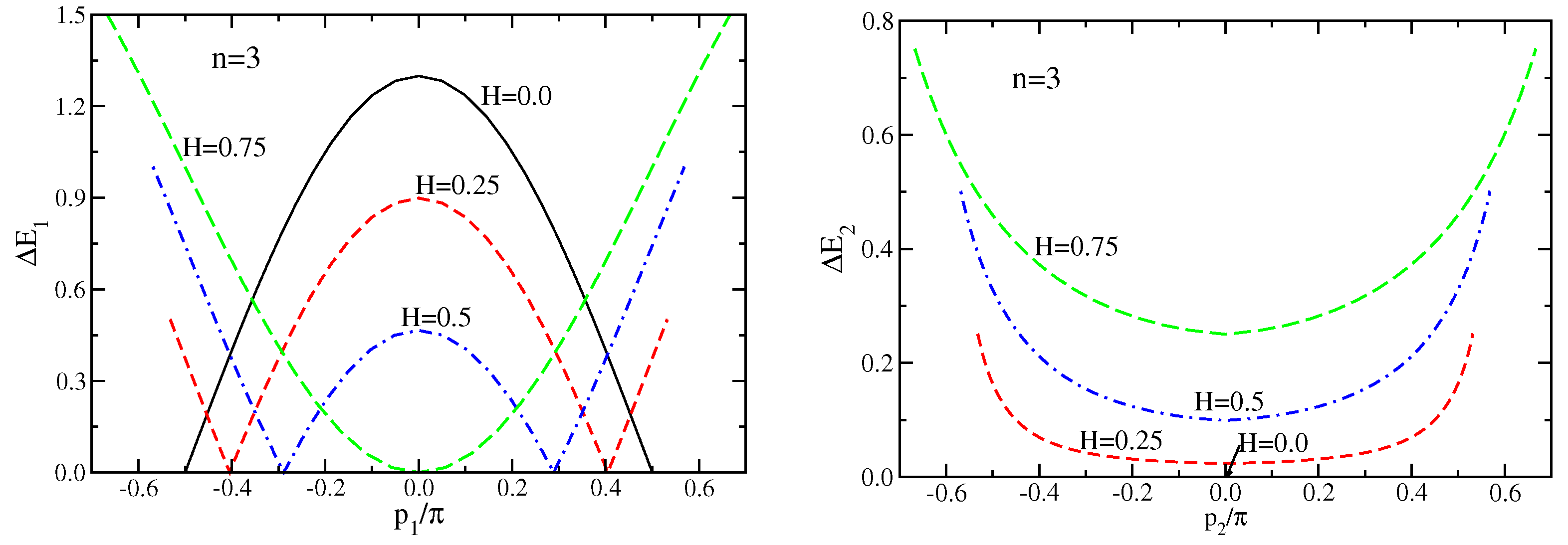
The dispersions for various fields are shown in Figure 2. In the left panel, the low-level energy dispersion, is presented. The zeroes of represent the Fermi points of the dispersions. The states are divided into particle and hole states. For the states are all particles and gapped (there is no Fermi momentum), while for all excitations are holes (see Figure 1). The range of the momenta increases with the magnetic field. For the second band (right panel) at , the dispersion reduces to a point and all states are empty.
3.2. Case
In this case, three bands are to be determined, , and , which satisfy the following equations
Analogously, the spinwave density functions and the momenta are given by
The dispersion functions for for various magnetic fields are displayed in Figure 3. The three panels show the three energy functions, , . Only the left upper panel () has Fermi points (zeroes of ) and has particle and hole states. All other excitations are particle-like, i.e., gapped (This is also the case for for ). Again the range of the momenta increases with the magnetic field. For the second and third bands at , the dispersion reduces to a point and all states are empty.
3.3. Case
For , the excitation spectra consist of four bands determined by the following equations
Similarly, the spinwave density functions and the momenta are obtain through
The dispersion functions for for various magnetic fields are displayed in Figure 4. The four panels show the four energy functions, , . Again only has Fermi points (zeroes of ) and has particle and hole states. All other excitations are particle-like, i.e., gapped (This is also the case for for ). As before, the range of the momenta increases with the magnetic field. For the second, third and fourth bands at the dispersion reduces to a point and all states are empty.
3.4. Luttinger Liquid
For a Luttinger liquid, the energy of the low-energy excitations is linearized in the momentum about the Fermi points. The spectrum can be described by the conformal tower in terms of four quantum numbers. The correlation functions, determined by the low-energy excitations of the system and the conformal space-time invariance, display power-law divergences. Conformal field theory only yields asymptotically exact correlation functions for long times and long distances, since the curvature of the dispersion is being neglected. These curvature terms in the Hamiltonian are formally irrelevant in the field theory [35], but modify the position of the singularity and the critical exponent.
In a series of papers [10,28,29,30,31,32,36,37,38,39,40,41,42], it was shown for several models that neglecting curvature terms in the dispersion leads to incorrect results for the threshold singularities in response functions. This problem is solved by adding a corrective term of the form of a mobile impurity that is coupled to the Luttinger liquid modes. Although formally irrelevant operators, the impurity terms, if treated nonperturbatively, yield the correct threshold singularities in the Green’s function. The method is not limited to weak interactions. The procedure is analogous to the X-ray edge divergence in metals [43,44], which arises from the perturbation of the Fermi surface when a core electron is promoted (the impurity). The exact critical exponents are determined by the scattering phase shifts off the impurity and for integrable models they can be extracted from the Bethe ansatz solution. Previous work on mobile impurities embedded into a Fermi gas should be mentioned [45,46,47,48,49,50,51,52,53,54]. However, in contrast to the present work, where the “impurity” is just an excitation of the interacting 1D system, there the impurity refers to a foreign particle dragging through the Luttinger liquid.
3.5. Group Velocities
In the Luttinger limit, where the dispersion of the excitations is linear in the momentum, the group velocity is given by [55]
where X separates particles from holes (Fermi point). The group velocity away from the linear dispersion regime is
where is the impurity rapidity. corresponds to the slope of the dispersion in Figure 1. Note that for hole-excitations in the Heisenberg chain, is always smaller than the respective Fermi velocity.
3.6. Conformal Towers
In the Luttinger limit, the model has excitations with energy proportional to the momentum with Fermi velocity . The finite size corrections to the ground state energy determine the energies of the low-lying excitations [56]. The ground state energy, , is an extensive quantity given by Equation (5). The excitations, on the other hand, are mesoscopic corrections, i.e., of order , where N is the length of the system. These mesoscopic corrections depend on the boundary conditions employed, in our case periodic boundary conditions. Four quantum numbers determine the finite size corrections, namely, corresponds to the number of removed or added rapidities and D is the parity variable, i.e., is the difference between the number of forward and backward movers. In addition, the quantum numbers count the number of particle and hole excitations about each Fermi point (+ for forward movers and − for backward movers). The ground state energy with finite size corrections is given by [56,57]
and assuming that the momentum of the ground state is zero, the excitations change the momentum by [57]
The quantity z in Equation (27) is the generalized dressed charge, which determines the interaction between the two Fermi points, i.e., how the energy is affected by a change of a quantum number, e.g., or D. The periodic boundary conditions for the discrete Bethe Ansatz equations restrict the values of the back-scattering quantum number D to be an integer. The dressed generalized charge is determined by , where is the solution of
Consider now a conformal field operator characterized by a set of quantum numbers , D and . The conformal dimensions, defined as [58,59]
determine the critical exponents of asymptotes of the correlation function. Conformal field theory then yields for the asymptote of
The correlation function consists of two factors corresponding to forward and backward movers, respectively. Each of these factors gives rise to a power-law singularity.
4. Field Theory Model for the Luttinger Liquid with Mobile Impurity
The field theory for the Luttinger liquid, i.e., the model with the linear dispersion in the momentum is parametrized by a Bose field, , and its dual field, , which satisfy the commutation relation [35]
The Luttinger liquid Hamiltonian is given by
where irrelevant operators have been neglected. Here K is the Luttinger parameter, which determines the strength of the interaction. For a noninteracting system .
The deviations from linearity of the dispersion lead in general to incorrect results in the threshold position and the exponents in response functions [10,29,30,32,36,38,39,41,42,60,61,62]. A high energy excitation from the nonlinear portion of the spectrum can be included by coupling the Luttinger liquid to a mobile impurity. This mobile impurity, if treated non-perturbatively, leads to singularities in the response function with the correct energy and momentum-dependent exponent.
A spinwave with energy added to the system is emulated by the following mobile impurity Hamiltonian (see, e.g., Refs. [10,29,30,36,39,41,62])
where and d are the creation and annihilation operators of the mobile impurity, is the momentum and u the group velocity of the excitation. The interaction of the Luttinger liquid with the mobile impurity is linear through coupling parameters and
In Section 5, the parameters in Equations (33)–(35) are related to quantities from the Bethe Ansatz.
We now consider and to eliminate the terms linear in the fields and we apply a canonical transformation U to all operators [10,29,30,32],
where the parameters and are to be determined. The transformed quantities are denoted by , and so that
The unwanted linear terms disappear if [10,29]
and the transformed Hamiltonian becomes noninteracting
As a consequence of the transformation, boundary terms are introduced for the boson fields, and , which are obtained by taking expectation values in Equation (37) [10]
where is the current quantum number (backscattering) and N the length of the chain.
5. Relation to the Bethe Ansatz Results
We now calculate the finite size corrections to the ground state energy in the presence of a high energy excitation using the Bethe Ansatz equations. The results for hole and particle excitations are similar, so that here we consider holes. Removing a rapidity introduces a small asymmetry in the integration limits, which are symmetric at without excitation. We denote the new integration limits with and .
5.1. Densities
The term with is the term of the excitation with the removed quantum number and . depends, in principle, on the size of the system, but its corrections are of order and hence negligible. With the aid of the Euler–MacLaurin sum formula the discrete equations can be transformed into an integral form for large M
The integration boundaries are fixed by , where with being the number of spinwaves in the ground state.
Dividing Equation (42) by and differentiating with respect to x the integral equation for for the finite system of length N is obtained. Expanding in powers of , i.e., , where represents the density of the bulk, is the impurity contribution and contains the finite size effects. Taking into account that , while , we have for
where is
and for the integration kernel we have [2]
which in the absence of a magnetic field yields .
The integral equation for is essentially the change in the density function due to a “hole” excitation, again except for the integration limits, i.e.,
Finally, the last driving terms in Equation (42) determine the integral equation for , i.e.,
5.2. Energy
In terms of discrete rapidities, the energy of the system with M spinwaves is given by
where is given by Equation (13).
Removing one spinwave of rapidity and employing once again the Euler–MacLaurin sum formula this expression reduces to [29,59]
Defining 50 ground state energy density in the thermodynamic limit is
and the energy of the finite system can be written as
where the prime denotes derivative. After a tedious calculation the -terms reduce to .
Next we simplify the impurity terms in the expression for the energy. The rapidity of the “impurity”, , is in principle dependent on the size of the system and can be expanded in powers of . The corrections to can, however, be neglected. The terms of order , i.e., the third and fourth terms in Equation (51), reduce to the dressed energy of the hole, , but with integration limits
The energy of the system is now given by
5.3. Integration Limits
The quantities are of the order of . We now expand to second order in these differences. The linear terms vanish, i.e., , because the excitations vanish at the Fermi points, i.e., . Hence, the first term corresponds to the equilibrium energy density in the ground state and the first corrections are quadratic,
After lengthy algebra we obtain
In summary, the corrections to the energy due to the finite size of the system are
5.4. Relation of to Quantum Numbers
The change of the integration limits due to the high energy excitation can be related to the quantum numbers of the excitation. The changes for the density and current density to order are obtained as
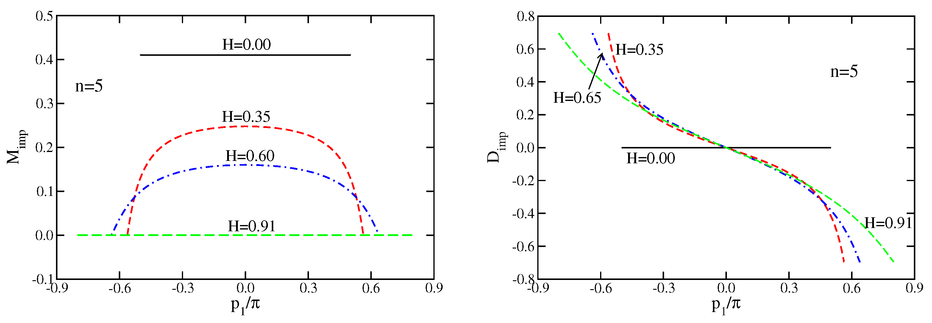
where is related to the impurity. We denote with and the quantities related to the high energy excitations (mobile impurities) (Figure 5, Figure 6 and Figure 7)
Note that we replaced the integration limits in Equation (58) by and that and do not necessarily vanish at the Fermi level. The shifts of with and to leading order in are given by and , respectively. It now follows that
Denoting with and , the corrections to the energy due to finite size take the form
All of the above considerations for “hole” excitations are straightforwardly extended to “particle” excitations.
5.5. Luttinger Parameter
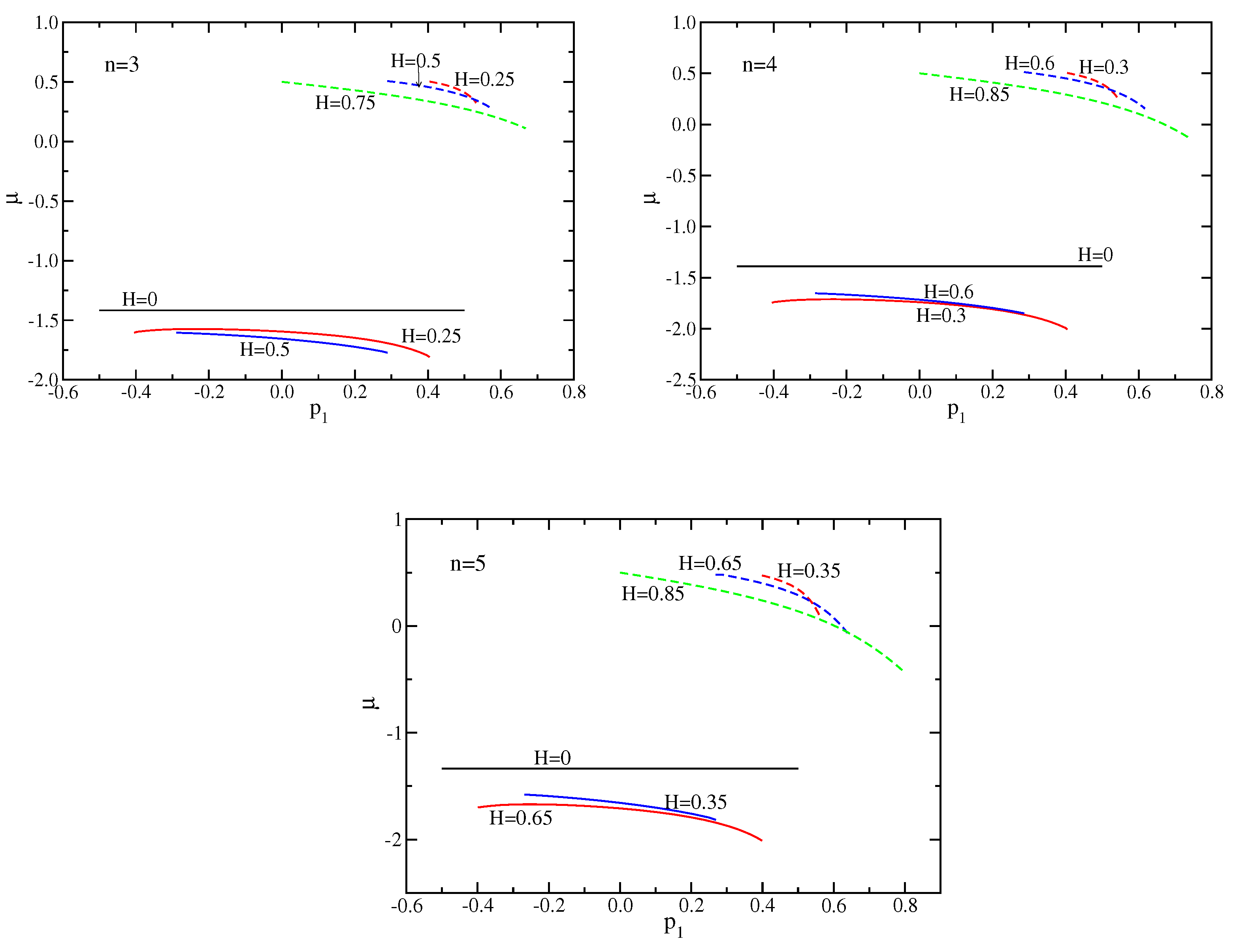
To parametrize the interaction strength in the field theory model for the Luttinger liquid, we need the Luttinger parameter K in terms of the Bethe ansatz quantities. To determine K, we consider the equal time spinwave propagator for which the quantum numbers are and . The correlation function decreases with a power law of the distance x, , where . This is in analogy to the Bose gas [41,63]. The field-theoretical approach yields through bosonization [11,12,64], so that . The quantity z is calculated via Equation (29) through the Bethe Ansatz as a function of field. z and K are displayed in Figure 8. The exact result for K at zero-field is [11,12]
5.6. Relation of the Bethe Ansatz with the Field Theoretical Quantities
We can now establish the relation between the field-theoretical and the Bethe Ansatz approaches. For simplicity we are going to consider spinwave “holes”, for which , . In Equation (40) the overlined quantities are proportional to and . It follows that
or inverting these equations we have
According to Refs. [39,62], the critical exponent for the hole excitation is
while for a particle excitation
The critical exponents for particles and holes, and , can now be evaluated and are shown in Figure 9.
Note that the exponent for the particles in the regime (close to the Fermi point) is always positive indicating a divergence of the spectral function, while the one for the holes is negative for and the spectral function tends to zero. For particles with , the exponent may change sign. Note that at the edge at the holes and particles are joined by an imaginary vertical line.
The spectral function is then proportional to the following general form
where with for particles and with for holes. As noted by Imambekov and Glazman [62] the exponents show markedly non-Luttinger liquid behavior in the immediate vicinity of the edges. For the Luttinger liquid and . Note that the conformal towers cannot give rise to a dependence [62]. The difference between the exact results and the Luttinger liquid arises from the fact that and are not zero at the Fermi surface.
6. Conclusions
We considered the excitation spectrum and edge singularities of the one-dimensional anisotropic Heisenberg chain for with and 5. Here corresponds to the X-Y chain (rotator model). The excitation spectrum consists of excitation bands. The model is integrable and the complete Bethe Ansatz solution was constructed by Takahashi and coworkers [20,22,24,25]. When is a rational number, the number of unknown functions in the Bethe Ansatz becomes finite, while if is an irrational number the Bethe Ansatz consists of an infinite number of unknown functions. This holds for antiferromagnetic exchange as well as for ferromagnetic coupling, . In the present paper we dealt with the antiferromagnetic case, while the critical behavior of the ferromagnetic situation was studied in Refs. [24,25]. The numerical solution of the isotropic ferromagnetic Heisenberg model (using a truncation method for large number of equations) yields a critical exponent of with logarithmic corrections [26,27]. The approach employed by Takahashi and Yamada [24,25] consists of the numerical solution of the Bethe Ansatz equations for , , and its extrapolation to . The results are and , in agreement with Schlottmann [26,27], except for the logarithmic corrections. Between rational numbers for are plenty of irrational numbers, which contain logarithmic terms and are skipped by the extrapolation method by Takahashi and Yamada. The validity of the extrapolation method is then questionable.
Using a combination of the Bethe Ansatz solution and field theory methods, we derived the spectral function for spinwave particle and hole excitations with high energy. In analogy to other models investigated previously [10,12,29,36,37,38,39,60,61,62], we consider an effective model consisting of the Luttinger liquid coupled to a mobile impurity to obtain the time-dependence of the single particle Green’s function. The parametrization of the high energy excited state as a mobile impurity allows to incorporate the exact excitation energy. Linearly coupling the impurity to the Luttinger liquid is analogous to the x-ray-threshold problem [43,44] and the arising power-law singularity in frequency or time is then the consequence of Anderson’s “infrared orthogonality catastrophy” [65]. As in Refs. [10,29,30,32,41], the mobile impurity is justified via the exact Bethe Ansatz solution of the model. The phenomenological parameters of the field theoretical model are this way determined from the Bethe Ansatz. The Luttinger liquid parameter K is related to the generalized dressed charge z (). In addition, we obtain from the Bethe Ansatz solution the exact energy of the excitation, and the momentum dependent scattering phase shifts.
We employed a procedure consisting of calculating the terms of the energy using the discrete Bethe Ansatz equations. The finite size corrections are evaluated for the system in the ground state including a high-energy particle or hole excitation. The conformal towers describe the low-energy excitations in a Luttinger liquid about the Fermi points. The present procedure extends the standard finite size terms to arbitrary excitations and consequently goes beyond the bosonization of spins and conformal field theory.
Funding
This research received no external funding.
Conflicts of Interest
The author declares no conflict of interest.
References
- Orbach, R. Linear antiferromagnetic chain with anisotropic coupling. Phys. Rev. 1958, 112, 309. [Google Scholar] [CrossRef]
- des Cloizeaux, J.; Gaudin, M. Anisotropic linear magnetic chain. J. Math. Phys. 1966, 7, 1384. [Google Scholar] [CrossRef]
- Yang, C.N.; Yang, C.P. One-dimensional chain of anisotropic spin-spin interactions. I. Proof of Bethe’s hypothesis for ground state in a finite system. Phys. Rev. 1966, 150, 321. [Google Scholar] [CrossRef]
- Yang, C.N.; Yang, C.P. One-dimensional chain of anisotropic spin-spin interactions. II. Properties of the ground-state energy per lattice site for an infinite system. Phys. Rev. 1966, 150, 327. [Google Scholar] [CrossRef]
- Yang, C.N.; Yang, C.P. One-dimensional chain of anisotropic spin-spin interactions. III. Applications. Phys. Rev. 1966, 151, 258. [Google Scholar] [CrossRef]
- Burkhardt, T.W.; Schlottmann, P. Edge pinning and internal phase transitions in a system of domain walls. Z. Phys. B 1984, 54, 151. [Google Scholar] [CrossRef]
- Burkhardt, T.W. Localisation-delocalisation transition in a solid-on-solid model with a pinning potential. J. Phys. A 1981, 14, L63. [Google Scholar] [CrossRef]
- Burkhardt, T.W.; Schlottmann, P. Unbinding transition in a many-string system. J. Phys. A 1993, 26, L501. [Google Scholar] [CrossRef]
- Caux, J.-S.; Maillet, J.M. Computation of dynamical correlation functions of Heisenberg chains in a magnetic field. Phys. Rev. Lett. 2005, 95, 077201. [Google Scholar] [CrossRef] [PubMed] [Green Version]
- Pereira, R.G.; Sirker, J.; Caux, J.-S.; Hagemans, R.; Maillet, J.M.; White, S.R.; Affleck, I. Dynamical spin structure factor for the anisotropic spin-1/2 Heisenberg chain. Phys. Rev. Lett. 2006, 96, 257202. [Google Scholar] [CrossRef] [PubMed]
- Pereira, R.G.; Sirker, J.; Caux, J.-S.; Hagemans, R.; Maillet, J.M.; White, S.R.; Affleck, I. Dynamical structure factor at small q for the XXZ spin-1/2 chain. J. Stat. Mech. 2007, P08022. [Google Scholar]
- Pereira, R.G.; White, S.R.; Affleck, I. Exact edge singularities and dynamical correlations in spin-1/2 chains. Phys. Rev. Lett. 2008, 100, 027206. [Google Scholar] [CrossRef] [PubMed] [Green Version]
- Pereira, R.G.; White, S.R.; Affleck, I. Spectral function of spinless fermions on a one-dimensional lattice. Phys. Rev. B 2009, 79, 165113. [Google Scholar] [CrossRef] [Green Version]
- Caux, J.-S.; Konno, H.; Sorrell, M.; Weston, R. Tracking the effects of interactions on spinons in gapless Heisenberg chains. Phys. Rev. Lett. 2011, 106, 217203. [Google Scholar] [CrossRef] [PubMed] [Green Version]
- Caux, J.-S.; Konno, H.; Sorrell, M.; Weston, R. Exact form-factor results for the longitudinal structure factor of the massless XXZ model in zero field. J. Stat. Mech. 2012, P01007. [Google Scholar] [CrossRef]
- Gaudin, M. Thermodynamics of the Heisenberg-Ising ring for δ≥1. Phys. Rev. Lett. 1971, 26, 1301. [Google Scholar] [CrossRef]
- Caux, J.-S.; Mossel, J.; Pérez Castillo, I. The two-spinon transverse structure factor of the gapped Heisenberg antiferromagnetic chain. J. Stat. Mech. 2008, P08006. [Google Scholar] [CrossRef] [Green Version]
- Carmelo, J.M.P.; Sacramento, P.D. The role of q-spin singlet pairs of physical spins in the dynamical properties of the spin-1/2 Heisenberg-Ising XXZ chain. Nucl. Phys. B 2022, 974, 115610. [Google Scholar] [CrossRef]
- Yang, W.; Wu, J.; Xu, S.; Wang, Z.; Wu, C. One-dimensional quantum spin dynamics of Bethe string states. Phys. Rev. B 2019, 100, 184406. [Google Scholar] [CrossRef] [Green Version]
- Takahashi, M.; Suzuki, M. One-dimensional anisotropic Heisenberg model at finite temperature. Prog. Theor. Phys. 1972, 48, 2187. [Google Scholar] [CrossRef] [Green Version]
- Takahashi, M. One-dimensional Heisenberg model at finite temperature. Prog. Theor. Phys. 1971, 46, 401. [Google Scholar] [CrossRef]
- Takahashi, M. Low-temperature specific heat of spin-1/2 anisotropic Heisenberg ring. Prog. Theor. Phys. 1973, 50, 1519. [Google Scholar] [CrossRef] [Green Version]
- Takahashi, M. Numerical calculation of thermodynamic quantities of spin-1/2 anisotropic Heisenberg ring. Prog. Theor. Phys. 1974, 51, 1348. [Google Scholar] [CrossRef] [Green Version]
- Takahashi, M.; Yamada, M. Spin-1/2 one-dimensional Heisenberg ferromagnet at low-temperature. J. Phys. Soc. Jpn. 1985, 54, 2808. [Google Scholar] [CrossRef]
- Yamada, M.; Takahashi, M. Critical behavior of spin-1/2 one-dimensional Heisenberg ferromagnet at low-temperature. J. Phys. Soc. Jpn. 1986, 55, 2024. [Google Scholar] [CrossRef]
- Schlottmann, P. Critical behavior of the isotropic ferromagnetic quantum Heisenberg chain. Phys. Rev. Lett. 1985, 54, 2131. [Google Scholar] [CrossRef]
- Schlottmann, P. Low temperature behavior of the S = 1/2 ferromagnetic Heisenberg chain. Phys. Rev. B 1986, 33, 4880. [Google Scholar] [CrossRef]
- Imambekov, A.; Glazman, L.I. Phenomenology of One-Dimensional Quantum Liquids Beyond the Low-Energy Limit. Phys. Rev. Lett. 2009, 102, 126405, Universal Theory of Nonlinear Luttinger Liquids. Science 2009, 323, 228.. [Google Scholar] [CrossRef] [Green Version]
- Essler, F.H.L. Threshold singularities in the one-dimensional Hubbard model. Phys. Rev. B 2010, 81, 205120. [Google Scholar] [CrossRef] [Green Version]
- Schlottmann, P.; Zvyagin, A.A. Threshold singularities in a Fermi gas with attractive potential in one dimension. Nucl. Phys. B 2015, 2015 892, 269. [Google Scholar] [CrossRef] [Green Version]
- Ovchinnikov, A.A. Threshold singularities in the correlators of the one-dimensional models. J. Stat. Mech. Theory Exp. 2016, 2016, 063108. [Google Scholar] [CrossRef]
- Schlottmann, P. Exponents of the spectral functions in the one-dimensional Bose gas. Condens. Matter 2018, 3, 35. [Google Scholar] [CrossRef] [Green Version]
- Lieb, E.H.; Schultz, T.D.; Mattis, D.C. Two soluble models of an antiferromagnetic chain. Ann. Phys. 1961, 16, 407. [Google Scholar] [CrossRef]
- Katsura, S. Statistical Mechanics of the Anisotropic Linear Heisenberg Model. Phys. Rev. 1962, 127, 1508. [Google Scholar] [CrossRef]
- Haldane, F.D.M. ‘Luttinger liquid theory’ of one-dimensional quantum fluids. I. Properties of the Luttinger model and their extension to the general 1D interacting spinless Fermi gas. J. Phys. C Solid State Phys. 1981, 14, 2585. [Google Scholar] [CrossRef]
- Khodas, M.; Pustilnik, M.; Kamenev, A.; Glazman, L.I. Dynamics of excitations in a one-dimensional Bose liquid. Phys. Rev. Lett. 2007, 99, 110405. [Google Scholar] [CrossRef] [Green Version]
- Khodas, M.; Pustilnik, M.; Kamenev, A.; Glazman, L.I. Fermi-Luttinger liquid: Spectral function of interacting one-dimensional fermions. Phys. Rev. B 2007, 76, 155402. [Google Scholar] [CrossRef] [Green Version]
- Cheianov, V.V.; Pustilnik, M. Threshold Singularities in the Dynamic Response of Gapless Integrable Models. Phys. Rev. Lett. 2008, 100, 126403. [Google Scholar] [CrossRef] [Green Version]
- Schmidt, T.L.; Imambekov, A.; Glazman, L.I. Fate of 1D Spin-Charge Separation Away from Fermi Points. Phys. Rev. Lett. 2010, 2010 104, 116403. [Google Scholar] [CrossRef] [Green Version]
- Imambekov, A.; Schmidt, T.L.; Glazman, L.I. One-dimensional quantum liquids: Beyond the Luttinger liquid paradigm. Rev. Mod. Phys. 2012, 84, 1253. [Google Scholar] [CrossRef] [Green Version]
- Schlottmann, P. Threshold singularities in the one-dimensional supersymmetric boson -fermion gas mixture. Int. J. Mod. Phys. B 2018, 32, 1850221. [Google Scholar] [CrossRef]
- Schlottmann, P. Edge singularities in the one-dimensional Bariev model. Nucl. Phys. B 2019, 949, 114808. [Google Scholar] [CrossRef]
- Noziéres, P.; de Dominicis, C.T. Singularities in the X-Ray Absorption and Emission of Metals. III. One-Body Theory Exact Solution. Phys. Rev. 1969, 178, 1097. [Google Scholar] [CrossRef]
- Schotte, K.D.; Schotte, U. Tomonaga’s Model and the Threshold Singularity of X-Ray Spectra of Metals. Phys. Rev. 1969, 182, 479. [Google Scholar] [CrossRef]
- Ogawa, T.; Furusaki, A.; Nagaosa, N. Fermi-edge singularity in one-dimensional systems. Phys. Rev. Lett. 1992, 68, 3638. [Google Scholar] [CrossRef]
- Castella, H.; Zotos, X. Exact calculation of spectral properties of a particle interacting with a one-dimensional fermionic system. Phys. Rev. B 1993, 47, 16186. [Google Scholar] [CrossRef] [PubMed] [Green Version]
- Sorella, S.; Parola, A. Spectral Properties of One Dimensional Insulators and Superconductors. Phys. Rev. Lett. 1996, 76, 4604. [Google Scholar] [CrossRef] [Green Version]
- Castro Neto, A.H.; Fisher, M.P.A. Dynamics of a heavy particle in a Luttinger liquid. Phys. Rev. B 1996, 53, 9713. [Google Scholar] [CrossRef] [Green Version]
- Tsukamoto, Y.; Fujii, T.; Kawakami, N. Critical behavior of Tomonaga-Luttinger liquids with a mobile impurity. Phys. Rev. B 1998, 58, 3633. [Google Scholar] [CrossRef]
- Schlottmann, P.; Zvyagin, A.A. Integrable supersymmetric t-J model with magnetic impurity. Phys. Rev. B 1997, 55, 5027. [Google Scholar] [CrossRef]
- Schlottmann, P.; Zvyagin, A.A. Exact solution for a degenerate Anderson impurity in the U→∞ limit embedded into a correlated host. Eur. Phys. J. B 1998, 5, 325. [Google Scholar] [CrossRef]
- Balents, L. X-ray-edge singularities in nanotubes and quantum wires with multiple subbands. Phys. Rev. B 2000, 61, 4429. [Google Scholar] [CrossRef] [Green Version]
- Friedrich, A.; Kolezhuk, A.K.; McCulloch, I.P.; Schollwöck, U. Edge singularities in high-energy spectra of gapped one-dimensional magnets in strong magnetic fields. Phys. Rev. B 2007, 75, 094414. [Google Scholar] [CrossRef] [Green Version]
- Burovski, E.; Cheianov, V.; Gamayun, O.; Lychkovskiy, O. Momentum relaxation of a mobile impurity in a one-dimensional quantum gas. Phys. Rev. A 2014, 89, 041601. [Google Scholar] [CrossRef] [Green Version]
- Lieb, E.H. Exact analysis of an interacting Bose gas. II. The excitation spectrum. Phys. Rev. 1963, 130, 1616. [Google Scholar] [CrossRef]
- Izergin, A.G.; Korepin, V.E.; Reshetikhin, N.Y. Conformal dimensions in Bethe ansatz solvable models. J. Phys. A Math. Gen. 1989, 22, 2615. [Google Scholar] [CrossRef]
- Schlottmann, P. Exact Results for Highly Correlated Electron Systems in One Dimension. Int. J. Mod. Phys. B 1997, 11, 355. [Google Scholar] [CrossRef]
- Frahm, H.; Korepin, V.E. Critical exponents for the one-dimensional Hubbard model. Phys. Rev. B 1990, 42, 10553. [Google Scholar] [CrossRef] [PubMed]
- Woynarovich, F. Finite-size effects in a non-half-filled Hubbard chain. J. Phys. A Math. Gen. 1989, 22, 4243. [Google Scholar] [CrossRef]
- Pustilnik, M.; Khodas, M.; Kamenev, A.; Glazman, L.I. Dynamic Response of One-Dimensional Interacting Fermions. Phys. Rev. Lett. 2006, 96, 196405. [Google Scholar] [CrossRef] [PubMed] [Green Version]
- Zvonarev, M.B.; Cheianov, V.V.; Giamarchi, T. Spin Dynamics in a One-Dimensional Ferromagnetic Bose Gas. Phys. Rev. Lett. 2007, 99, 240404. [Google Scholar] [CrossRef] [PubMed]
- Imambekov, A.; Glazman, L.I. Exact Exponents of Edge Singularities in Dynamic Correlation Functions of 1D Bose Gas. Phys. Rev. Lett. 2008, 100, 206805. [Google Scholar] [CrossRef] [Green Version]
- Frahm, H.; Palacios, G. Correlation functions of one-dimensional Bose-Fermi mixtures. Phys. Rev. A 2005, 72, 061604. [Google Scholar] [CrossRef] [Green Version]
- Cazalilla, M.A. Bosonizing one-dimensional cold atomic gases. J. Phys. B At. Mol. Opt. Phys. 2004, 37, S1. [Google Scholar] [CrossRef]
- Anderson, P.W. Infrared catastrophe in Fermi gases with local scattering potentials. Phys. Rev. Lett. 1967, 18, 1049. [Google Scholar] [CrossRef]
Figure 1.
(Color online) Elementary spinwave excitations as a function of the momentum for and three values of n: (black, solid) , (red, dashed) , and (blue, dash-dotted) . and are the energy and momentum of the first band (ground state band), which is half-filled.
Figure 1.
(Color online) Elementary spinwave excitations as a function of the momentum for and three values of n: (black, solid) , (red, dashed) , and (blue, dash-dotted) . and are the energy and momentum of the first band (ground state band), which is half-filled.
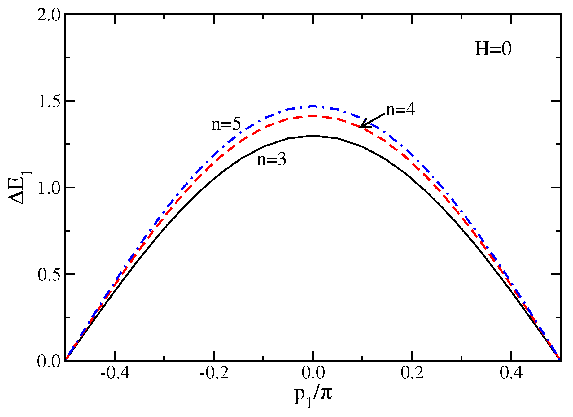
Figure 2.
(Color online) Spinwave excitations for for several fields ( black solid line; red dashed line; blue dash-dotted line; green long-dashed line). (left panel) : The Fermi momentum is defined as the zero of for each H. Hole excitations correspond to , while particle excitations to . The range of increases with H. For the excitations are gapped and have no Fermi point. (right panel) : The excitation energies are gapped, except for , where the dispersion reduces to a single point. All states are empty in this case.

Figure 3.
(Color online) Spinwave excitations for for several fields ( black solid line; red dashed line; blue dash-dotted line; green long-dashed line). (left upper panel) : The Fermi momentum is defined as the zero of for each H. Hole excitations correspond to , while particle excitations to . The range of increases with H. For the excitations are gapped and have no Fermi point. (right upper panel) : The excitation energies are gapped, except for , where the dispersion reduces to a single point and all states are empty in this case. (lower panel) : For the third band, the dispersion again reduces to a point for .

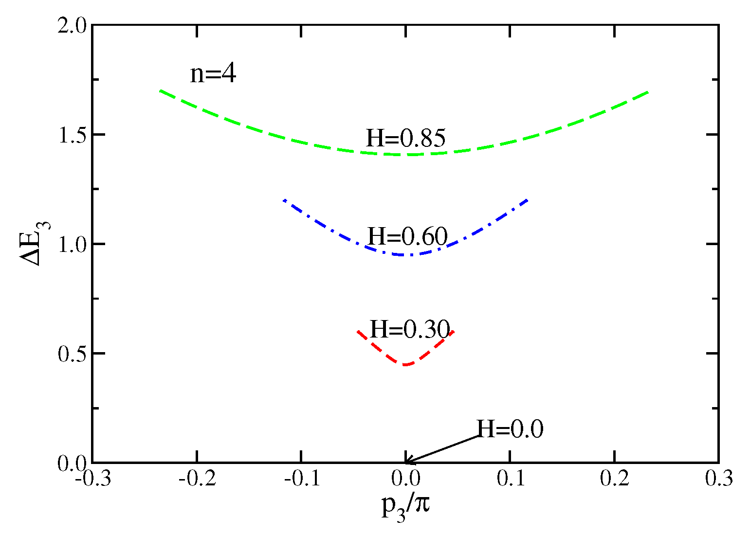
Figure 4.
(Color online) Spinwave excitations for for several fields ( black solid line; red dashed line; blue dash-dotted line; green long-dashed line). (left top panel) : The Fermi momentum is defined as the zero of for each H. Hole excitations correspond to , while particle excitations to . The range of increases with H. For the excitations are gapped and have no Fermi point. (right top panel) : The excitation energies are gapped, except for , where the dispersion reduces to a single point and all states are empty in this case. (lower left panel) : For the third band the dispersion again reduces to a point for . (lower right panel) : Similar to and .
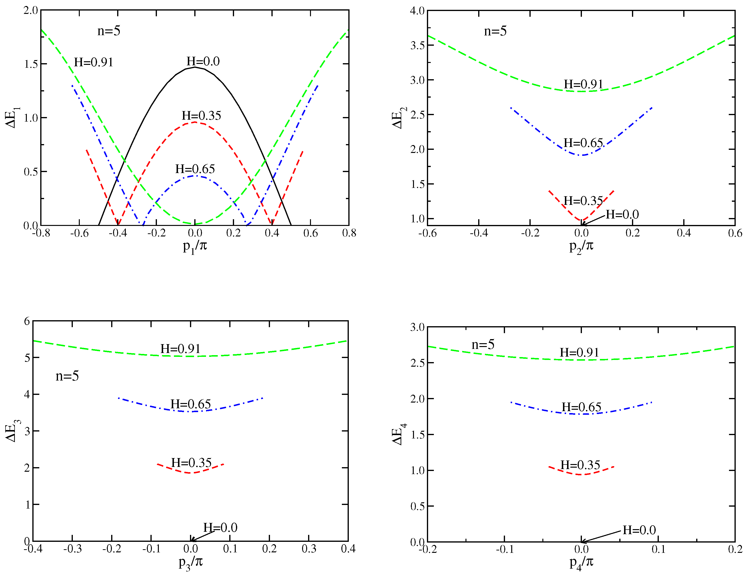
Figure 5.
(Color online) (left panel) “Impurity” density and (right panel) current density as a function of the momentum for a high energy excitation for . Note that is an even function of the momentum and is an odd function of the momentum.
Figure 5.
(Color online) (left panel) “Impurity” density and (right panel) current density as a function of the momentum for a high energy excitation for . Note that is an even function of the momentum and is an odd function of the momentum.
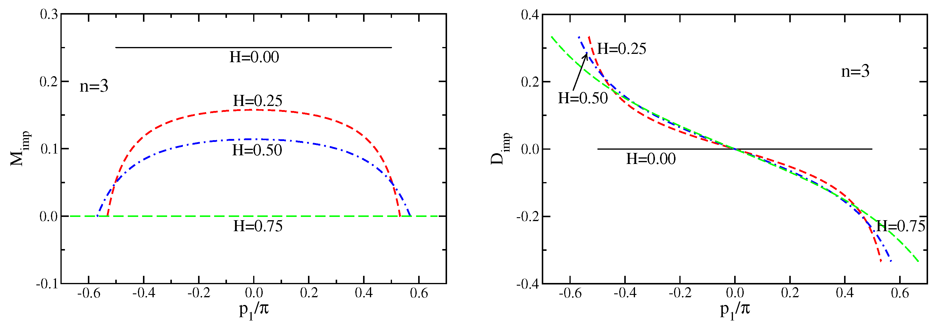
Figure 6.
(Color online) (left panel) “Impurity” density and (right panel) current density as a function of the momentum for a high energy excitation for . Note that is an even function of the momentum and is an odd function of the momentum.
Figure 6.
(Color online) (left panel) “Impurity” density and (right panel) current density as a function of the momentum for a high energy excitation for . Note that is an even function of the momentum and is an odd function of the momentum.

Figure 7.
(Color online) (left panel) “Impurity” density and (right panel) current density as a function of the momentum for a high energy excitation for . Note that is an even function of the momentum and is an odd function of the momentum.
Figure 7.
(Color online) (left panel) “Impurity” density and (right panel) current density as a function of the momentum for a high energy excitation for . Note that is an even function of the momentum and is an odd function of the momentum.

Figure 8.
Dressed generalized charge z (solid lines) and the Luttinger parameter (dashed lines) as a function of magnetic field for (black), (red) and (blue).
Figure 8.
Dressed generalized charge z (solid lines) and the Luttinger parameter (dashed lines) as a function of magnetic field for (black), (red) and (blue).

Figure 9.
(Color online) Critical exponents of the spectral function of spinwaves as a function of momentum for particles (, dashed curves) and holes (, solid curves) for (upper left panel), (upper right panel) and (lower panel). The same magnetic fields as in previous figures are considered. The exponents for holes are always negative and the spectral function tends to zero. On the other hand, the exponents for particles are positive at the edge and hence the spectral function diverges. Away from may change sign and become negative.

Publisher’s Note: MDPI stays neutral with regard to jurisdictional claims in published maps and institutional affiliations. |
© 2022 by the author. Licensee MDPI, Basel, Switzerland. This article is an open access article distributed under the terms and conditions of the Creative Commons Attribution (CC BY) license (https://creativecommons.org/licenses/by/4.0/).
Share and Cite
MDPI and ACS Style
Schlottmann, P. Excitation Spectra and Edge Singularities in the One-Dimensional Anisotropic Heisenberg Model for Δ = cos(π/n), n = 3,4,5. Quantum Rep. 2022, 4, 442-461. https://doi.org/10.3390/quantum4040032
AMA Style
Schlottmann P. Excitation Spectra and Edge Singularities in the One-Dimensional Anisotropic Heisenberg Model for Δ = cos(π/n), n = 3,4,5. Quantum Reports. 2022; 4(4):442-461. https://doi.org/10.3390/quantum4040032
Chicago/Turabian StyleSchlottmann, Pedro. 2022. "Excitation Spectra and Edge Singularities in the One-Dimensional Anisotropic Heisenberg Model for Δ = cos(π/n), n = 3,4,5" Quantum Reports 4, no. 4: 442-461. https://doi.org/10.3390/quantum4040032